The Link between Default and Recovery Rates: Theory, Empirical ...

Edward I. Altman 

Stern School of Business, New York University 

Brooks Brady 

Standard and Poor’s 

Andrea Resti 

Bocconi University, Italy 

Andrea Sironi 

Bocconi University, Milan 

The Link between Default 

and Recovery Rates: Theory, 

Empirical Evidence, 

and Implications* 

I. Introduction 

Credit risk affects virtually every financial contract. 

Therefore the measurement, pricing, and management 

of credit risk have received much attention 

from financial economists, bank supervisors and 

regulators, and financial market practitioners. Following 

the recent attempts of the Basel Committee 

on Banking Supervision (1999, 2001) to reform 

the capital adequacy framework by introducing 

risk-sensitive capital requirements, significant 

* This paper is a significant extension of a report prepared for 

the International Swaps and Dealers Association (ISDA; 2000). 

We thank ISDA for its financial and intellectual support. We 

thank Richard Herring, Hiroshi Nakaso, and the other participants 

at the BIS conference (March 6, 2002) on ‘‘Changes in Risk 

through Time: Measurement and Policy Options’’ (London) for 

their useful comments. The paper also profited by the comments 

from participants in the CEMFI (Madrid, Spain) Workshop 

on April 2, 2002, especially Rafael Repullo, Enrique Sentana, 

and Jose Campa; from workshops at the Stern School of Business 

(NYU), University of Antwerp, University of Verona, and 

Bocconi University; and from an anonymous reviewer. 

(Journal of Business, 2005, vol. 78, no. 6) 

B 2005 by The University of Chicago. All rights reserved. 

0021-9398/2005/7806-0006$10.00 

This paper analyzes the 

association between 

default and recovery 

rates on credit assets 

and seeks to empirically 

explain this critical 

relationship. We 

examine recovery rates 

on corporate bond 

defaults over the period 

1982–2002. Our 

econometric univariate 

and multivariate models 

explain a significant 

portion of the variance 

in bond recovery rates 

aggregated across 

seniority and collateral 

levels. We find that 

recovery rates are a 

function of supply 

and demand for the 

securities, with default 

rates playing a pivotal 

role. Our results have 

important implications 

for credit risk models 

and for the procyclicality 

effects of the New Basel 

Capital Accord. 

2203

2204 Journal of Business 

additional attention has been devoted to the subject of credit risk measurement 

by the international regulatory, academic, and banking communities. 

This paper analyzes and measures the association between aggregate 

default and recovery rates on corporate bonds and seeks to empirically 

explain this critical relationship. After a brief review of the way credit 

risk models explicitly or implicitly treat the recovery rate variable, 

Section III examines the recovery rates on corporate bond defaults over 

the period 1982–2002. We attempt to explain recovery rates by specifying 

rather straightforward linear, logarithmic, and logistic regression 

models. The central thesis is that aggregate recovery rates are basically 

a function of supply and demand for the securities. Our econometric 

univariate and multivariate time-series models explain a significant portion 

of the variance in bond recovery rates aggregated across all seniority 

and collateral levels. In Sections IV and V, we briefly examine 

the effects of the relationship between defaults and recoveries on credit 

VaR (value at risk) models and the procyclicality effects of the new 

capital requirements proposed by the Basel Committee, then conclude 

with some remarks on the general relevance of our results. 

II. The Relationship between Default Rates and Recovery Rates in Credit 

Risk Modeling: A Review of the Literature 

Credit risk models can be divided into three main categories: (1) ‘‘first 

generation’’ structural-form models, (2) ‘‘second generation’’ structuralform 

models, and (3) reduced-form models. Rather than go through a 

discussion of each of these well-known approaches and their advocates in 

the literature, we refer the reader to our earlier report for ISDA (Altman, 

Resti, and Sironi 2001), which carefully reviews the literature on the 

conceptual relationship between the firm’s probability of default (PD) and 

the recovery rate (RR) after default to creditors. 1 

During the last few years, new approaches explicitly modeling and 

empirically investigating the relationship between PD and RR have been 

developed. These include Frye (2000a, 2000b), Jokivuolle and Peura 

(2003), and Jarrow (2001). The model proposed by Frye draws from the 

conditional approach suggested by Finger (1999) and Gordy (2000). In 

these models, defaults are driven by a single systematic factor–the state 

of the economy–rather than by a multitude of correlation parameters. 

The same economic conditions are assumed to cause defaults to rise, for 

example, and RRs to decline. The correlation between these two variables 

therefore derives from their common dependence on the systematic 

factor. The intuition behind Frye’s theoretical model is relatively simple: 

if a borrower defaults on a loan, a bank’s recovery may depend on the 

value of the loan collateral. The value of the collateral, like the value of 

1. See Altman, Resti and Sironi (2001) for a formal discussion of this relationship.

Default and Recovery Rates 

2205 

other assets, depends on economic conditions. If the economy experiences 

a recession, RRs may decrease just as default rates tend to increase. 

This gives rise to a negative correlation between default rates and RRs. 

The model originally developed by Frye (2000a) implied recovery from 

an equation that determines collateral. His evidence is consistent with the 

most recent U.S. bond market data, indicating a simultaneous increase in 

default rates and losses given default (LGDs) 2 in 1999–2001. 3 Frye’s 

(2000b, 2000c) empirical analysis allows him to conclude that, in a 

severe economic downturn, bond recoveries might decline 20–25 percentage 

points from their normal-year average. Loan recoveries may 

decline by a similar amount but from a higher level. 

Jarrow (2001) presents a new methodology for estimating RRs and 

PDs implicit in both debt and equity prices. As in Frye (2000a, 2000b), 

RRs and PDs are correlated and depend on the state of the economy. However, 

Jarrow’s methodology explicitly incorporates equity prices in the estimation 

procedure, allowing the separate identification of RRs and PDs 

and the use of an expanded and relevant data set. In addition, the methodology 

explicitly incorporates a liquidity premium in the estimation procedure, 

which is considered essential in the light of the high variability in 

the yield spreads between risky debt and U.S. Treasury securities. 

A rather different approach is proposed by Jokivuolle and Peura 

(2000). The authors present a model for bank loans in which collateral 

value is correlated with the PD. They use the option pricing framework 

for modeling risky debt: the borrowing firm’s total asset value determines 

the event of default. However, the firm’s asset value does not 

determine the RR. Rather, the collateral value is in turn assumed to be 

the only stochastic element determining recovery. Because of this assumption, 

the model can be implemented using an exogenous PD, so that 

the firm’s asset value parameters need not be estimated. In this respect, 

the model combines features of both structural-form and reduced-form 

models. Assuming a positive correlation between a firm’s asset value and 

collateral value, the authors obtain a result similar to Frye (2000a), that 

realized default rates and recovery rates have an inverse relationship. 

Using Moody’s historical bond market data, Hu and Perraudin (2002) 

examine the dependence between recovery rates and default rates. They 

first standardize the quarterly recovery data to filter out the volatility of 

recovery rates given by the variation over time in the pool of borrowers 

rated by Moody’s. They find that correlations between quarterly 

recovery rates and default rates for bonds issued by U.S.-domiciled 

2. LGD indicates the amount actually lost (by an investor or a bank) for each dollar lent 

to a defaulted borrower. Accordingly, LGD and RR always add to 1. One may also factor 

into the loss calculation the last coupon payment, which is usually not realized when a 

default occurs (see Altman 1989). 

3. Gupton, Hamilton, and Berthault (2001) provide clear empirical evidence of this 

phenomenon.


obligors are 0.22 for post 1982 data (1983–2000) and 0.19 for the 

1971–2000 period. Using extreme value theory and other nonparametric 

techniques, they also examine the impact of this negative correlation 

on credit VaR measures and find that the increase is statistically 

significant when confidence levels exceed 99%. 

Bakshi, Madan, and Zhang (2001) enhance the reduced-form models 

presented earlier to allow for a flexible correlation between the riskfree 

rate, the default probability, and the recovery rate. Based on some 

preliminary evidence published by rating agencies, they force recovery 

rates to be negatively associated with default probability. They find some 

strong support for this hypothesis through the analysis of a sample of 

BBB-rated corporate bonds: more precisely, their empirical results show 

that, on average, a 4% worsening in the (risk-neutral) hazard rate is associated 

with a 1% decline in (risk-neutral) recovery rates. 

Compared to the aforementioned contributions, our study extends 

the existing literature in three main directions. First, the determinants 

of defaulted bonds’ recovery rates are empirically investigated. While 

most of the aforementioned recent studies concluded in favor of an 

inverse relationship between these two variables, based on the common 

dependence on the state of the economy, none of them empirically 

analyzed the more specific determinants of recovery rates. While our 

analysis shows empirical results that appear consistent with the intuition 

of a negative correlation between default rates and RRs, we find that a 

single systematic risk factor (the performance of the economy) is less 

predictive than the aforementioned theoretical models would suggest. 

Second, our study is the first one to examine, both theoretically and 

empirically, the role played by supply and demand of defaulted bonds in 

determining aggregate recovery rates. Our econometric univariate and 

multivariate models assign a key role to the supply of defaulted bonds and 

show that these variables together with variables that proxy the size of the 

high-yield bond market explain a substantial proportion of the variance in 

bond recovery rates aggregated across all seniority and collateral levels. 

Third, our simulations show the consequences the negative correlation 

between default and recovery rates would have on VaR models and 

the procyclicality effect of the capital requirements recently proposed 

by the Basel Committee. Indeed, while our results on the impact of this 

correlation on credit risk measures (such as unexpected loss and value at 

risk) are in line with the ones obtained by Hu and Perraudin (2002), they 

show that, if a positive correlation highlighted by bond data were to be 

confirmed by bank data, the procyclicality effects of ‘‘Basel II’’ might 

be even more severe than expected if banks use their own estimates of 

LGD. Indeed, the Basel Commission assigned a task force in 2004 to 

analyze ‘‘recoveries in downturns’’ in order to assess the significance of a 

decrease in activity on LGD. A report was issued in July 2005 with some 

guidelines for banks ({ 468 of the framework document).


2207 

As concerns specifically the Hu and Perraudin paper, it should be 

pointed out that they correlate recovery rates (or percent of par, which is 

the same thing) with issuer-based default rates. Our models assess the 

relationship between dollar-denominated default and recovery rates and, 

as such, can assess directly the supply/demand aspects of the defaulted 

debt market. Moreover, in addition to assessing the relationship between 

default and recovery rates using ex post default rates, we explore the effect 

of using ex ante estimates of the future default rates (i.e., default probabilities) 

instead of actual, realized defaults. As will be shown, however, 

while the negative relationship between RR and both ex post and ex ante 

default rates is empirically confirmed, the probabilities of default show a 

considerably lower explanatory power. Finally, it should be emphasized 

that, while our paper and the one by Hu and Perraudin reach similar 

conclusions, albeit from very different approaches and tests, it is important 

that these results become accepted and are subsequently reflected 

in future credit risk models and public policy debates and regulations. 

For these reasons, concurrent confirming evidence from several sources 

are beneficial, especially if they are helpful in specifying fairly precisely 

the default rate/recovery rate nexus. 

III. Explaining Aggregate Recovery Rates on Corporate Bond Defaults: 

Empirical Results 

The average loss experience on credit assets is well documented in 

studies by the various rating agencies (Moody’s, S&P, and Fitch) as 

well as by academics. 4 Recovery rates have been observed for bonds, 

stratified by seniority, as well as for bank loans. The latter asset class can 

be further stratified by capital structure and collateral type (Van de 

Castle and Keisman 2000). While quite informative, these studies say 

nothing about the recovery versus default correlation. The purpose of 

this section is to empirically test this relationship with actual default 

data from the U.S. corporate bond market over the last two decades. As 

pointed out in Section II, strong intuition suggests that default and 

recovery rates might be correlated. Accordingly, this section of our 

study attempts to explain the link between the two variables, by specifying 

rather straightforward statistical models. 5 

We measure aggregate annual bond recovery rates (henceforth, BRR) 

by the weighted average recovery of all corporate bond defaults, primarily 

4. See, e.g., Altman and Kishore (1996), Altman and Arman (2002), FITCH (1997, 

2001), Standard & Poor’s (2000). 

5. We will concentrate on average annual recovery rates but not on the factors that contribute 

to understanding and explaining recovery rates on individual firm and issue defaults. 

Unal, Madan, and Güntay (2003) propose a model for estimating risk-neutral expected recovery 

rate distributions, not empirically observable rates. The latter can be particularly useful 

in determining prices on credit derivative instruments, such as credit default swaps.


in the United States, over the period 1982–2001. The weights are based on 

the market value of defaulting debt issues of publicly traded corporate 

bonds. 6 The logarithm of BRR (BLRR) is also analyzed. 

The sample includes annual and quarterly averages from about 1,300 

defaulted bonds for which we were able to get reliable quotes on the price 

of these securities just after default. We utilize the database constructed 

and maintained by the NYU Salomon Center, under the direction of one 

of the authors. Our models are both univariate and multivariate least 

squares regressions. The univariate structures can explain up to 60% of 

the variation of average annual recovery rates, while the multivariate 

models explain as much as 90%. 

The rest of this section proceeds as follows. We begin our analysis by 

describing the independent variables used to explain the annual variation 

in recovery rates. These include supply-side aggregate variables that are 

specific to the market for corporate bonds, as well as macroeconomic 

factors (some demand-side factors, like the return on distressed bonds 

and the size of the ‘‘vulture’’ funds market, are discussed later). Next, we 

describe the results of the univariate analysis. We then present our multivariate 

models, discussing the main results and some robustness checks. 

A. Explanatory Variables 

We proceed by listing several variables we reasoned could be correlated 

with aggregate recovery rates. The expected effects of these variables 

on recovery rates will be indicated by a + or sign in parentheses. The 

exact definitions of the variables we use are: 

BDR( ). The weighted average default rate on bonds in the 

high-yield bond market and its logarithm (BLDR, ( )). 

Weights are based on the face value of all high-yield bonds 

outstanding each year and the size of each defaulting 

issue within a particular year. 7 

6. Prices of defaulted bonds are based on the closing ‘‘bid’’ levels on or as close to the 

default date as possible. Precise-date pricing was possible only in the last 10 years or so, 

since market maker quotes were not available from the NYU Salomon Center database prior 

to 1990 and all prior date prices were acquired from secondary sources, primarily the S&P 

Bond Guides. Those latter prices were based on end-of-month closing bid prices only. We 

feel that more exact pricing is a virtue, since we are trying to capture supply and demand dynamics, 

which may affect prices negatively if some bondholders decide to sell their defaulted 

securities as fast as possible. In reality, we do not believe this is an important factor, since 

many investors will have sold their holdings prior to default or are more deliberate in their 

‘‘dumping’’ of defaulting issues. 

7. We did not include a variable that measures the distressed but not defaulted proportion 

of the high-yield market, since we do not know of a time-series measure that goes back to 

1987. We define distressed issues as yielding more than 1,000 basis points over the risk-free 

10-year Treasury bond rate. We did utilize the average yield spread in the market and found 

it was highly correlated (0.67) to the subsequent 1-year’s default rate, hence it did not add 

value (see the discussion later). The high-yield bond yield spread, however, can be quite 

helpful in forecasting the following year’s BDR, a critical variable in our model (see our 

discussion of a default probability prediction model in Section III.F).


2209 

BDRC( ). The 1-year change in BDR. 

BOA( ). The total amount of high-yield bonds outstanding for 

a particular year (measured at midyear in trillions of 

dollars), which represents the potential supply of 

defaulted securities. Since the size of the high-yield 

market has grown in most years over the sample period, 

the BOA variable picks up a time-series trend as well 

as representing a potential supply factor. 

BDA( ). We also examined the more directly related bond 

defaulted amount as an alternative for BOA 

(also measured in trillions of dollars). 

GDP(+). The annual GDP growth rate. 

GDPC(+). The change in the annual GDP growth rate from the 

previous year. 

GDPI( ). Takes the value of 1 when GDP growth was less than 

1.5% and 0 when GDP growth was greater than 1.5%. 

SR(+). 

SCR(+). 

The annual return on the S&P 500 stock index. 

The change in the annual return on the S&P 500 stock 

index from the previous year. 

B. The Basic Explanatory Variable: Default Rates 

It is clear that the supply of defaulted bonds is most vividly depicted by 

the aggregate amount of defaults and the rate of default. Since virtually 

all public defaults most immediately migrate to default from the noninvestment 

grade or ‘‘junk’’ bond segment of the market, we use that 

market as our population base. The default rate is the par value of defaulting 

bonds divided by the total amount outstanding, measured at face 

values. Table 1 shows default rate data from 1982–2001, as well as the 

weighted average annual recovery rates (our dependent variable) and the 

default loss rate (last column). Note that the average annual recovery is 

41.8% (weighted average 37.2%) and the weighted average annual loss 

rate to investors is 3.16%. 8 The correlation between the default rate and 

the weighted price after default amounts to 0.75. 

C. The Demand and Supply of Distressed Securities 

The logic behind our demand/supply analysis is both intuitive and important, 

especially since, as we have seen, most credit risk models do not 

formally and statistically consider this relationship. On a macroeconomic 

8. The loss rate is affected by the lost coupon at default as well as the more important lost 

principal. The 1987 default rate and recovery rate statistics do not include the massive Texaco 

default, since it was motivated by a lawsuit which was considered frivolous, resulting in a 

strategic bankruptcy filing and a recovery rate (price at default) of over 80%. Including Texaco 

would have increased the default rate by over 4% and the recovery rate to 82% (reflecting the 

huge difference between the market’s assessment of asset values versus liabilities, not typical 

of bankrupt companies). The results of our models would be less impressive, although still 

quite significant, with Texaco included.


TABLE 1 

Default Rates, Recovery Rates, and Losses 

Year 

Par Value 

Outstanding 

(a) 

($million) 

Par Value 

of Defaults 

(b) 

($million) 

Default 

Rate 

Weighted Price 

after Default 

(Recovery 

Rate) 

Weighted 

Coupon 

Default Loss 

(c) 

2001 $649,000 $63,609 9.80% 25.5 9.18% 7.76% 

2000 $597,200 $30,295 5.07% 26.4 8.54% 3.95% 

1999 $567,400 $23,532 4.15% 27.9 10.55% 3.21% 

1998 $465,500 $7,464 1.60% 35.9 9.46% 1.10% 

1997 $335,400 $4,200 1.25% 54.2 11.87% .65% 

1996 $271,000 $3,336 1.23% 51.9 8.92% .65% 

1995 $240,000 $4,551 1.90% 40.6 11.83% 1.24% 

1994 $235,000 $3,418 1.45% 39.4 10.25% .96% 

1993 $206,907 $2,287 1.11% 56.6 12.98% .56% 

1992 $163,000 $5,545 3.40% 50.1 12.32% 1.91% 

1991 $183,600 $18,862 10.27% 36.0 11.59% 7.16% 

1990 $181,000 $18,354 10.14% 23.4 12.94% 8.42% 

1989 $189,258 $8,110 4.29% 38.3 13.40% 2.93% 

1988 $148,187 $3,944 2.66% 43.6 11.91% 1.66% 

1987 $129,557 $1,736 1.34% 62.0 12.07% .59% 

1986 $90,243 $3,156 3.50% 34.5 10.61% 2.48% 

1985 $58,088 $992 1.71% 45.9 13.69% 1.04% 

1984 $40,939 $344 .84% 48.6 12.23% .48% 

1983 $27,492 $301 1.09% 55.7 10.11% .54% 

1982 $18,109 $577 3.19% 38.6 9.61% 2.11% 

Weighted 

average 4.19% 37.2 10.60% 3.16% 

Note.—Default rate data from 1982–2001 are shown, as well as the weighted average annual 

recovery rates and the loss rates. The time series show a high correlation (75%) between default and 

recovery rates. 

(a) Measured at mid-year, excludes defaulted issues. 

(b) Does not include Texaco’s bankruptcy in 1987. 

(c) Includes lost coupon as well as principal loss. 

Source: Authors’ compilations. 

level, forces that cause default rates to increase during periods of economic 

stress also cause the value of assets of distressed companies to 

decrease. Hence the securities’ values of these companies will likely be 

lower. While the economic logic is clear, the statistical relationship between 

GDP variables and recovery rates is less significant than what one 

might expect. We hypothesized that, if one drills down to the distressed 

firm market and its particular securities, we can expect a more significant 

and robust negative relationship between default and recovery rates. 9 

9. Consider the latest highly stressful period of corporate bond defaults in 2000–02. The 

huge supply of bankrupt firms’ assets in sectors like telecommunications, airlines, and steel, to 

name a few, has had a dramatic negative impact on the value of the firms in these sectors as they 

filed for bankruptcy and attempted a reorganization under Chapter 11. Altman and Jha (2003) 

estimated that the size of the U.S. distressed and defaulted public and private debt markets 

swelled from about $300 billion (face value) at the end of 1999 to about $940 billion by yearend 

2002. And, only 1 year in that 3-year period was officially a recession year (2001). As we 

will show, the recovery rate on bonds defaulting in this period was unusually low as telecom 

equipment, large body aircraft, and steel assets of distressed firms piled up.


2211 

The principal purchasers of defaulted securities, primarily bonds and 

bank loans, are niche investors called distressed asset or alternative 

investment managers, also called vultures. Prior to 1990, there was little 

or no analytic interest in these investors, indeed in the distressed debt 

market, except for the occasional anecdotal evidence of performance in 

such securities. Altman (1991) was the first to attempt an analysis of the 

size and performance of the distressed debt market and estimated, based 

on a fairly inclusive survey, that the amount of funds under management 

by these so-called vultures was at least $7.0 billion in 1990 and, if you 

include those investors who did not respond to the survey and nondedicated 

investors, the total was probably in the $10–12 billion range. 

Cambridge Associates (2001) estimated that the amount of distressed 

assets under management in 1991 was $6.3 billion. Estimates since 

1990 indicate that the demand did not rise materially until 2000–01, 

when the estimate of total demand for distressed securities was about 

$40–45 billion as of December 31, 2001 and $60–65 billion 1 year later 

(see Altman and Jha 2003). So, while the demand for distressed securities 

grew slowly in the 1990s and early in the next decade, the supply 

(as we will show) grew enormously. 

On the supply side, the last decade has seen the amounts of distressed 

and defaulted public and private bonds and bank loans grow dramatically 

in 1990–91 to as much as $300 billion (face value) and $200 

billion (market value), then recede to much lower levels in the 1993–98 

period, and grow enormously again in 2000–02 to the unprecedented 

levels of $940 billion (face value) and almost $500 billion market 

value as of December 2002. These estimates are based on calculations 

in Altman and Jha (2003) from periodic market calculations and 

estimates. 10 

On a relative scale, the ratio of supply to demand of distressed and 

defaulted securities was something like 10 to 1 in both 1990–91 and 

2000–01. Dollarwise, of course, the amount of supply-side money 

dwarfed the demand in both periods. And, as we will show, the price 

levels of new defaulting securities was relatively very low in both periods, 

at the start of the 1990s and again at the start of the 2000 decade. 

D. Univariate Models 

We begin the discussion of our results with the univariate relationships 

between recovery rates and the explanatory variables described in the 

previous section. Table 2 displays the results of the univariate regressions 

10. Defaulted bonds and bank loans are relatively easy to define and are carefully documented 

by the rating agencies and others. Distressed securities are defined here as bonds 

selling at least 1,000 basis points over comparable maturity Treasury bonds (we use the 

10-year T-bond rate as our benchmark). Privately owned securities, primarily bank loans, are 

estimated as 1.4–1.8 the level of publicly owned distressed and defaulted securities based 

on studies of a large sample of bankrupt companies (Altman and Jha 2003).

TABLE 2 

Univariate Regressions, 1982–2001: Variables Explaining Annual Recovery Rates on Defaulted Corporate Bonds 

A. Market Variables 

Regression number 1 2 3 4 5 6 7 8 9 10 

Dependent variable 

BRR X X X X X 

BLLR X X X X X 

Explanatory variables: coefficients and (t-ratios) 

Constant .509 .668 .002 1.983 .432 .872 .493 .706 .468 .772 

(18.43) ( 10.1) (.03) ( 10.6) (24.9) ( 20.1) (13.8) ( 8.05) (19.10) ( 13.2) 

BDR 2.610 6.919 

( 4.36) ( 4.82) 

BLDR .113 .293 

( 5.53) ( 5.84) 

BDRC 3.104 7.958 

( 4.79) ( 4.92) 

BOA .315 .853 

( 2.68) ( 2.95) 

BDA 4.761 13.122 

( 3.51) ( 4.08) 

Goodness of fit measures 

R 2 .514 .563 .630 .654 .560 .574 .286 .326 .406 .481 

Adjusted r 2 .487 .539 .609 .635 .536 .550 .246 .288 .373 .452 

F-statistic 19.03 23.19 30.61 34.06 22.92 24.22 7.21 8.69 12.31 16.67 

( p-value) .000 .000 .000 .000 .000 .000 .015 .009 .003 .001 

Residual tests 

Serial correlation LM, 2 lags (Breusch-Godfrey) 1.021 1.836 1.522 2.295 1.366 2.981 1.559 1.855 3.443 2.994 

( p-value) .600 .399 .467 .317 .505 .225 .459 .396 .179 .224 

Heteroscedasticity (White, Chi square) .089 1.585 .118 1.342 8.011 5.526 2.389 1.827 .282 1.506 

( p-value) .956 .453 .943 .511 .018 .063 .303 .401 .868 .471 

N. obs. 20 20 20 20 20 20 20 20 20 20 

2212 Journal of Business

B. Macro Variables 

Regression # 11 12 13 14 15 16 17 18 19 20 

Dependent variable 

BRR X X X X X 

BLRR X X X X X 

Explanatory variables 

Constant .364 1.044 .419 .907 .458 .804 .387 1.009 .418 .910 

(7.59) ( 8.58) (18.47) ( 15.65) (15.42) ( 10.8) (10.71) ( 11.3) (16.42) ( 14.4) 

GDP 1.688 4.218 

(1.30) (1.28) 

GDPC 2.167 5.323 

(2.31) (2.22) 

GDPI .101 .265 

( 2.16) ( 2.25) 

SR .205 .666 

(1.16) (1.53) 

SRC .095 .346 

(.73) (1.07) 


R 2 .086 .083 .228 .215 .206 .220 .070 .115 .029 .060 

Adjusted R 2 .035 .032 .186 .171 .162 .176 .018 .066 .025 .007 

F-statistic 1.69 1.64 5.33 4.93 4.66 5.07 1.36 2.35 .53 1.14 

( p-value) .211 .217 .033 .040 .045 .037 .259 .143 .475 .299 


Serial correlation LM, 2 lags (Breusch-Godfrey) 2.641 4.059 .663 1.418 .352 1.153 3.980 5.222 3.479 4.615 

( p-value) .267 .131 .718 .492 .839 .562 .137 .073 .176 .100 

Heteroscedasticity (White, Chi square) 2.305 2.077 2.254 2.494 .050 .726 2.515 3.563 3.511 4.979 

( p-value) .316 .354 .324 .287 .823 .394 .284 .168 .173 .083 

Number of observations 20 20 20 20 20 20 20 20 20 20 

Note.—The table shows the results of a set of univariate regressions carried out between the recovery rate (BRR) or its natural log (BLRR) and an array of explanatory 

variables: the default rate (BDR), its log (BLDR), and its change (BDRC); the outstanding amount of bonds (BOA) and the outstanding amount of defaulted bonds (BDA); the 

GDP growth rate (GDP), its change (GDPC), and a dummy (GDPI) taking the value of 1 when the GDP growth is less than 1.5%; the S&P 500 stock-market index (SR) and its 

change (SRC). 


2213


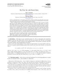
Fig. 1.—Univariate models. Results of a set of univariate regressions carried 

out between the recovery rate (BRR) or its natural log (BLRR) and the default 

rate (BDR) or its natural log (BLDR). See table 2 for more details. 

carried out using these variables. These univariate regressions, and the 

multivariate regressions discussed in the following section, were calculated 

using both the recovery rate (BRR) and its natural log (BLRR) as 

the dependent variables. Both results are displayed in table 2, as signified 

by an X in the corresponding row. 

We examined the simple relationship between bond recovery rates 

and bond default rates for the period 1982–2001. Table 2 and figure 1 

show several regressions between the two fundamental variables. We 

find that one can explain about 51% of the variation in the annual recovery 

rate with the level of default rates (this is the linear model, 

regression 1) and 60% or more with the logarithmic and power 11 relationships 

(regressions 3 and 4). Hence, our basic thesis that the rate of 

default is a massive indicator of the likely average recovery rate among 

corporate bonds appears to be substantiated. 12 

The other univariate results show the correct sign for each coefficient, 

but not all of the relationships are significant. BDRC is highly 

11. The power relationship (BRR ¼ e b0 BDR b1 ) can be estimated using the following 

equivalent equation: BLRR ¼ b 0 þ b 1 BLDR (‘‘power model’’). 

12. Such an impression is strongly supported by a 80% rank correlation coefficient 

between BDR and BRR (computed over the 1982–2001 period). Note that rank correlations 

represent quite a robust indicator, since they do not depend upon any specific functional 

form (e.g., log, quadratic, power).


2215 

TABLE 3 

Correlation Coefficients among the Main Variables 

BDR BOA BDA GDP SR BRR 

BDR 1.00 .33 .73 .56 .30 .72 

BOA 1.00 .76 .05 .21 .53 

BDA 1.00 .26 .49 .64 

GDP 1.00 .02 .29 

SR 1.00 .26 

BRR 1.00 

Note.—The table shows cross-correlations among our regressors (and between each of them and the 

recovery rate BRR); values greater than 0.5 are italicized. A strong link between GDP and BDR emerges, 

suggesting that default rates, as expected, are positively correlated with macro growth measures. 

negatively correlated with recovery rates, as shown by the very significant 

t-ratios, although the t-ratios and R 2 values are not as significant 

as those for BLDR. Both BOA and BDA, as expected, are negatively 

correlated with recovery rates, with BDA being more significant on a 

univariate basis. Macroeconomic variables do not explain as much of 

the variation in recovery rates as the corporate bond market variables; 

their poorer performance is also confirmed by the presence of some 

heteroscedasticity and serial correlation in the regression’s residuals, 

hinting at one or more omitted variables. We will come back to these 

relationships in the next paragraphs. 

E. Multivariate Models 

We now specify some more complex models to explain recovery rates, 

by adding several variables to the default rate. The basic structure of our 

most successful models is 

BRR ¼ f ðBDR; BDRC; BOA; or BDAÞ 

Some macroeconomic variables will be added to this basic structure, 

to test their effect on recovery rates. 

Before we move on to the multivariate results, table 3 reports the crosscorrelations 

among our regressors (and between each of them and the 

recovery rate, BRR); values greater than 0.5 are highlighted. A rather 

strong link between GDP and BDR emerges, suggesting that, as expected, 

default rates are positively correlated with macro growth measures. Hence, 

adding GDP to the BDR/BRR relationship is expected to blur the significance 

of the results. We also observe a high positive correlation between 

BDA (absolute amount of all defaulted bonds) and the default rate. 

We estimate our regressions using 1982–2001 data to explain recovery 

rate results and predict 2002 rates. This involves linear and loglinear 

structures for the two key variables, recovery rates (dependent) 

and default rates (explanatory), with the log-linear relationships somewhat 

more significant. These results appear in table 4.

TABLE 4 Multivariate Regressions, 1982–2001 

Linear and Logarithmic Models 

Logistic Models 

Regression 

number 1 2 3 4 5 6 7 8 9 10 11 12 13 14 15 

Dependent 

variable 

BRR X X X X X X X X X X 

BLRR X X X X X 

Explanatory 

variables: 

coefficients 

and (t-ratios) 

Constant .514 .646 .207 1.436 .482 1.467 .529 1.538 .509 1.447 .074 .097 .042 .000 .000 

(19.96) ( 11.34) (2.78) ( 8.70) (20.02) ( 6.35) (11.86) ( 9.07) (14.65) ( 8.85) ( .64) ( .92) (.44) (.00) (.00) 

BDR 1.358 3.745 1.209 1.513 1.332 12.200 6.713 5.346 7.421 6.487 

( 2.52) ( 3.13) ( 1.59) ( 2.28) ( 2.33) (4.14) (2.82) (1.55) (2.59) (2.64) 

BLDR .069 .176 .167 .222 .169 

( 3.78) ( 4.36) ( 2.94) ( 4.64) ( 4.17) 

BDRC 1.930 4.702 1.748 4.389 2.039 4.522 1.937 4.415 1.935 4.378 8.231 8.637 8.304 8.394 

( 3.18) ( 3.50) ( 3.39) ( 3.84) ( 3.03) ( 3.35) ( 3.11) ( 4.05) ( 3.09) ( 3.87) (3.339) (3.147) (3.282) (3.315) 

BOA .164 .459 .141 .410 .153 .328 .162 .387 .742 .691 .736 

( 2.13) ( 2.71) ( 2.12) ( 2.78) ( 1.86) ( 2.20) ( 2.03) ( 2.63) (2.214) (1.927) (2.136) 

BDA 1.203 3.199 8.196 

( .81) ( 1.12) (1.064) 

GDP .387 2.690 1.709 

( .43) ( 1.62) (.473) 

SR .020 .213 .242 

(.192) (1.156) ( .56) 

2216 Journal of Business

Goodness of 

fit measures 

R 2 .764 .819 .826 .867 .708 .817 .767 .886 .764 .878 .534 .783 .732 .786 .787 

Adjusted R 2 .720 .785 .793 .842 .654 .782 .704 .856 .702 .845 .508 .742 .682 .729 .731 

F-stat 17.250 24.166 25.275 34.666 12.960 23.752 12.320 29.245 12.168 26.881 20.635 19.220 14.559 13.773 13.876 

( p-value) .000 .000 .000 .000 .000 .000 .000 .000 .000 .000 .000 .000 .000 .000 .000 


Serial correlation 

LM, 2 lags 

(Breusch- 

Godfrey) 3.291 2.007 1.136 .718 1.235 .217 3.344 .028 5.606 1.897 1.042 2.673 1.954 2.648 5.899 

( p-value) .193 .367 .567 .698 .539 .897 .188 .986 .061 .387 .594 .263 .376 .266 .052 

Heteroscedasticity 

(White, 

Chi square) 5.221 5.761 5.049 5.288 12.317 12.795 5.563 4.853 6.101 6.886 .008 5.566 9.963 5.735 5.948 

( p-value) .516 .451 .538 .507 .055 .046 .696 .773 .636 .549 .996 .474 .126 .677 .653 

Numbers of 

observations 20 20 20 20 20 20 20 20 20 20 20 20 20 20 20 


Note.—The table shows the results of a set of multivariate regressions based on 1982–2001 data. Regressions 1 through 6 build the ‘‘basic models’’: most variables are quite 

significant based on their t-ratios. The overall accuracy of the fit goes from 71% (65% adjusted R 2 ) to 87% (84% adjusted); the model with the highest explanatory power and lowest 

‘‘error’’ rates is the power model in regression 4. Macroeconomic variables are added in columns 7–10, showing a poor explanatory power. A set of logistic estimates (cols. 11–15) is 

provided, to account for the fact that the dependent variable (recovery rates) is bounded between 0 and 1. 

2217


Regressions 1 through 6 build the ‘‘basic models’’: most variables are 

quite significant based on their t-ratios. The overall accuracy of the fit 

goes from 71% (65% adjusted R 2 ) to 87% (84% adjusted). 

The actual model with the highest explanatory power and lowest 

‘‘error’’ rates is the power model 13 in regression 4 of table 4. We see that 

all of the four explanatory variables have the expected negative sign and 

are significant at the 5% or 1% level. BLDR and BDRC are extremely 

significant, showing that the level and change in the default rate are highly 

important explanatory variables for recovery rates. Indeed, the variables 

BDR and BDRC explain up to 80% (unadjusted) and 78% (adjusted) of 

the variation in BRR based simply on a linear or log-linear association. 

The size of the high-yield market also performs very well and adds about 

6–7% to the explanatory power of the model. When we substitute BDA 

for BOA (regressions 5 and 6), the latter does not look statistically significant, 

and the R 2 of the multivariate model drops slightly to 0.82 (unadjusted) 

and 0.78 (adjusted). Still, the sign of BDA is correct (+). Recall 

that BDA was more significant than BOA on a univariate basis (table 2). 

Macro variables are added in columns 7–10: we are somewhat surprised 

by the low contributions of these variables since several models 

have been constructed that utilize macro variables, apparently significantly, 

in explaining annual default rates. 14 

As concerns the growth rate in annual GDP, the univariate analyses 

presented in tables 2 and 3 had shown it to be significantly negatively 

correlated with the bond default rate ( 0.78, see table 3); however, the 

univariate correlation between recovery rates (both BRR and BLRR) 

and GDP growth is relatively low (see table 2), although with the appropriate 

sign (+). Note that, when we utilize the change in GDP growth 

(GDPC, table 2, regression 5 and 6), the significance improves markedly. 

When we introduce GDP to our existing multivariate structures 

(table 4, regressions 7 and 8), not only is it not significant, but it has 

a counterintuitive sign (negative). The GDPC variable leads to similar 

results (not reported). No doubt, the high negative correlation between 

GDP and BDR reduces the possibility of using both in the same multivariate 

structure. 

We also postulated that the return of the stock market could affect 

the prices of defaulting bonds in that the stock market represented 

investor expectations about the future. A positive stock market outlook 

could imply lower default rates and higher recovery rates. For example, 

earnings of all companies, including distressed ones, could be reflected 

13. Like its univariate cousin, the multivariate power model can be written using logs: 

e.g., BLRR ¼ b 0 þ b 1 BLDR þ b 2 BDRC þ b 3 BOA becomes BRR ¼ exp ½b 0 Š 

BDR b1 exp ½b 2 BDRC þ b 3 BOAŠ and takes its name from BDR being raised to the 

power of its coefficient. 

14. See, e.g., Jonsson and Fridson (1996), Fridson, Garman, and Wu (1997), Helwege and 

Kleiman (1997), Keenan, Sobehart, and Hamilton (1999), and Chacko and Mercier (2001).


2219 

in higher stock prices. Table 4, regressions 9 and 10, show the association 

between the annual S&P 500 Index stock return (SR) and recovery 

rates. Note the insignificant t-ratios in the multivariate model, despite 

the appropriate signs. Similar results (together with low values of R 2 ) 

emerge from our univariate analysis (table 2), where the change in the 

S&Preturn(SRC)wasalsotested. 

Since the dependent variable (BRR) in most of our regressions is 

bounded by 0 and 1, we also ran the same models using a logistic 

function (table 4, columns 11–15). As can be seen, R 2 and t-ratios are 

broadly similar to those already shown. The model in column 12, including 

BDR, BDRC, and BOA, explains as much as 74% (adjusted R 2 ) 

of the recovery rate’s total variability. Macroeconomic variables, as 

before, tend to have no evident effect on BDR. 

F. Robustness Checks 

This section hosts some robustness checks carried out to verify how our 

results would change when taking into account several important modifications 

to our approach. 

Default probabilities. The models shown previously are based on 

the actual default rate experienced in the high yield, speculative-grade 

market (BDR) and reflect a coincident supply/demand dynamic in that 

market. One might argue that this ex post analysis is conceptually 

different from the specification of an ex ante estimate of the default 

rate. 

We believe both specifications are important. Our previous ex post 

models and tests are critical in understanding the actual experience of 

credit losses and, as such, affect credit management regulation and 

supervision, capital allocations, and credit policy and planning of financial 

institutions. On the other hand, ex ante probabilities (PDs) are 

customarily used in VaR models in particular and for risk-management 

purposes in general; however, their use in a regression analysis of recovery 

rates might lead to empirical tests that are inevitably limited by 

the models used to estimate PDs and their own biases. The results of 

these tests might therefore not be indicative of the true relationship 

between default and recovery rates. 

To assess the relationship between ex ante PDs and BRRs, we used 

PDs generated through a well-established default rate forecasting model 

from Moody’s (Keenan et al. 1999). This econometric model is used to 

forecast the global speculative grade issuer default rate and was fairly 

accurate (R 2 = 0.8) in its explanatory model tests. 15 

15. Thus far, Moody’s has tested its forecasts for the 36-month period 1999–2001 and 

found that the correlation between estimated (PD) and actual default rates was greater than 

0.90 (Hamilton et al. 2003). So, it appears that there can be a highly correlated link between 

estimated PDs and actual BDRs. By association, therefore, one can infer that accurate PD 

models can be used to estimate recovery rates and LGD.


The results of using Moody’s model to explain our recovery rates 

did demonstrate a significant negative relationship but the explanatory 

power of the multivariate models was considerably lower (adjusted R 2 = 

0.39), although still impressive with significant t-tests for the change in 

PD and the amount of bonds outstanding (all variables had the expected 

sign). Note that, since the Moody’s model is for global issuers and our 

earlier tests are for U.S.-dollar-denominated high-yield bonds, we did 

not expect that their PD model would be nearly as accurate in explaining 

U.S. recovery rates. 

Quarterly Data. Our results are based on yearly values, so we wanted 

to make sure that higher-frequency data would confirm the existence 

of a link between default rates and recoveries. Based on quarterly data, 16 

a simple, univariate estimate (see table 5) shows that (1) BDR is still 

strongly significant and shows the expected sign; (2) R 2 looks relatively 

modest (23.9% versus 51.4% for the annual data), because quarterly 

default rates and recovery rates tend to be very volatile (due to some 

‘‘poor’’ quarters with only very few defaults). 

Using a moving average of 4 quarters (BRR4W, weighted by the 

number of defaulted issues), we estimated another model (using BDR, 

its lagged value and its square, see the last column in table 5), obtaining 

amuchbetterR 2 (72.4%). This suggests that the link between default 

rates and recovery is somewhat ‘‘sticky’’ and, although confirmed by 

quarterly data, is better appreciated over a longer time interval. 17 Note 

that the signs of the coefficients behave as expected; for example, an 

increase in quarterly BDRs from 1% to 3% reduces the expected recovery 

rate from 39% to 31% within the same quarter, while a further 

decrease to 29% takes place in the following 3 months. 

Risk-free rates. We considered the role of risk-free rates in explaining 

recovery rates, since these, in turn, depend on the discounted cash 

flows expected from the defaulted bonds. We therefore added to our 

‘‘best’’ models (e.g., columns 3 and 4 in table 4) some ‘‘rate’’ variables 

(namely, the 1-year and 10-year U.S. dollar Treasury rates taken from 

the Federal Reserve Board of Governors, the corresponding discount 

rates, or alternatively, the ‘‘steepness’’ of the yield curve, as measured 

by the difference between 10-year and 1-year rates). The results are disappointing, 

since none of these variables ever is statistically significant 

at the 10% level. 18 

16. We had to refrain from using monthly data simply because of missing values (several 

months show no defaults, so it is impossible to compute recovery rates when defaulted bonds 

amount to zero). 

17. This is confirmed by the equation residuals, which look substantially autocorrelated. 

18. This might also be because one of our regressors (BOA, the amount of outstanding 

bonds) indirectly accounts for the level of risk-free rates, since lower rates imply higher 

market values and vice versa. Even removing BOA, however, risk-free rates cannot be found 

to be significant inside our model.


2221 

TABLE 5 Quarterly Regressions, 1990–2002 

Dependent Variable BRR BRR4W 

Explanatory variables: coefficients and (t-ratios) 

Constant 45.48 (17.61) 48.12 (39.3) 

BDR 5.77 ( 3.92) 8.07 ( 4.24) 

BDR( 1) 2.62 ( 2.87) 

BDRSQ 1.10 (2.87) 


R 2 .239 .724 

Adjusted R 2 .223 .705 

F-stat 15.36 38.47 

( p-value) .000 .000 


Serial correlation LM, 2 lags (Breusch-Godfrey) 1.129 10.456 

( p-value) .332 .000 

Heteroscedasticity (White, Chi square) 4.857 1.161 

( p-value) .012 .344 

Number of observations 51 48 

Note.—The table shows univariate estimates based on quarterly data. It appears that (1) BDR is 

strongly significant and has the expected sign; (2) R 2 looks relatively modest, because quarterly default 

rates and recovery rates tend to be very volatile; (3) expressing recovery rates as the moving average of 

four quarterly data (BRR4W) improves R 2 , suggesting that the link between default rates and recovery 

is somewhat ‘‘sticky.’’ 

Returns on defaulted bonds. We examined whether the return experienced 

by the defaulted bond market affects the demand for distressed 

securities, thereby influencing the ‘‘equilibrium price’’ of defaulted bonds. 

To do so, we considered the 1-year return on the Altman-NYU Salomon 

Center Index of Defaulted Bonds (BIR), a monthly indicator of the market-weighted 

average performance of a sample of defaulted publicly 

traded bonds. 19 This is a measure of the price changes of existing defaulted 

issues as well as the ‘‘entry value’’ of new defaults and, as such, is affected 

by supply and demand conditions in this ‘‘niche’’ market. 20 On a univariate 

basis, the BIR shows the expected sign (+) with a t-ratio of 2.67 and 

explains 35% of the variation in BRR. However, when BIR is included in 

multivariate models, its sign remains correct, but the marginal significance 

is usually below 10%. 

Outliers. The limited width of the time series on which our coefficient 

estimates are based suggests that they might be affected by a small 

number of outliers. We checked for this by eliminating 10% of the 

observations, choosing those associated with the highest residuals, 21 

19. More details can be found in Altman (1991) and Altman and Jha (2003). Note that we 

use a different time frame in our analysis (1987–2001), because the defaulted bond index 

return (BIR) has been calculated only since 1987. 

20. We are aware that the average recovery rate on newly defaulted bond issues could 

influence the level of the defaulted bond index and vice versa. The vast majority of issues in 

the index, however, usually comprise bonds that have defaulted in prior periods. And, as we 

will see, while this variable is significant on an univariate basis and does improve the overall 

explanatory power of the model, it is not an important contributor. 

21. This amounts to 2 years out of 20, namely, 1987 and 1997.


and running our regressions again. The results (not reported to save 

room) totally confirm the estimates shown in table 4. For example, for 

model 3, the coefficients associated with BLDR ( 0.15), BDRC 

( 4.26), and BOA ( 0.45) are virtually unchanged, and remain significant 

at the 1% level; the same happens for model 4 (the coefficients 

being, respectively, 0.15, 4.26, and 0.45). 

GDP dummy and regime effects. We saw, in our multivariate results, 

that the GDP variable lacks statistical significance and tends to have a 

counterintuitive sign when added to multivariate models. The fact that 

GDP growth is highly correlated with default rates, our primary explanatory 

variable, looks like a sensible explanation for this phenomenon. 

To try to circumvent this problem, we used a technique similar to 

Helwege and Kleiman (1997): they postulate that, while a change in 

GDP of say 1% or 2% was not very meaningful in explaining default 

rates when the base year was in a strong economic growth period, the 

same change was meaningful when the new level was in a weak economy. 

Following their approach, we built a dummy variable (GDPI) 

which takes the value of 1 when GDP grows at less than 1.5% and 0 

otherwise. The univariate GDPI results show a somewhat significant 

relationship with the appropriate negative sign (table 2); however, when 

one adds the ‘‘dummy’’ variable GDPI to the multivariate models discussed 

previously, the results (not reported) show no statistically significant 

effect, although the sign remains appropriate. 

We further checked whether the relationship between default rates and 

recoveries outlined in table 4 experiences a structural change depending 

on the economy being in a ‘‘good’’ or ‘‘bad’’ regime. To do so, we reestimated 

equations 1–4 in the table after removing recession years 

(simply defined as years showing a negative real GDP growth rate); the 

results (not reported), widely confirmed the results shown in table 4; this 

suggests that our original estimates are not affected by recession periods. 

Seniority and original rating. Our study considers default rates and 

recoveries at an aggregate level. However, to strengthen our analysis 

and get some further insights on the PD/LGD relationship, we also considered 

recovery rates broken down by seniority status and original rating. 

Table 6 shows the results obtained on such data for our basic univariate, 

translog model. One can see that the link between recovery rates 

and default frequencies remains statistically significant for all seniority 

and rating groups. However, such a link tends to be somewhat weaker 

for subordinated bonds and junk issues. Moreover, while the sensitivity 

of BRR to the default rate looks similar for both seniority classes, recovery 

rates on investment-grade bonds seem to react more steeply to 

changes in the default rate. In other words, the price of defaulted bonds 

with an original rating between AAA and BBB decreases more sharply 

as defaults become relatively more frequent. Perhaps the reason for 

this is that original issue investment grade defaults tend to be larger than


2223 

TABLE 6 

Univariate Regressions on Data Broken by Seniority Status 

and Original Rating 

Data Broken by 

Seniority Status 

Data Broken by 

Original Rating y 

Dependent Variable 

RR on 

Senior* 

Bonds 

(Log) 

RR on 

Subordinated** 

Bonds 

(Log) 

RR on 

Investment-Grade 

Bonds 

(Log) 

RR on 

Junk z 

Bonds 

(Log) 

Explanatory variables: 

coefficients and (t-ratios) 

Constant 2.97 2.58 2.70 2.70 

(13.91) (8.79) (9.77) (10.99) 

BLDR .24 .23 .31 .23 

( 4.30) ( 2.90) ( 4.16) ( 3.41) 


R 2 .507 .319 .519 .421 

Adjusted R 2 .479 .281 .489 .385 

F-statistic 18.487 8.431 17.291 11.652 

( p-value) .000 .009 .001 .004 


Serial correlation LM, 2 lags 

( Breusch-Godfrey) .6674 1.66 4.0302 .162 

( p-value) .5268 .2213 .0415 .852 

Heteroskedasticity 

(White, Chi square) .719 .2001 .4858 .4811 

( p-value) .5015 .8205 .6245 .6273 

Number of observations 20 20 18 18 

Note.—The table shows a set of univariate regressions, based on recovery rates broken down by 

seniority status and original rating. The link between recovery rates and default frequencies remains 

statistically significant for all seniority and rating groups. However, it grows weaker for subordinated 

bonds and junk issues. Moreover, recovery rates on investment-grade bonds seem to react more steeply 

to changes in the default rate. 

* Senior-secured and senior-unsecured bonds. 

** Senior-subordinated, subordinated, and discount bonds. 

y Years 1993 and 1994 are not included because no default took place on investment-grade issues. 

z Including unrated bonds. 

noninvestment-grade failures and the larger amounts of distressed assets 

depresses the recovery rates even greater in difficult periods. 

IV. Implications for Credit VaR Models, Capital Ratios, 

and Procyclicality 

The results of our empirical tests have important implications for a 

number of credit-risk-related conceptual and practical areas. This section 

reviews two key areas that can be affected significantly when one 

factors in that, in fact, default rates are negatively correlated with recovery 

rates. These are (1) credit VaR models and (2) the potential impact 

of our findings on the procyclicality of capital requirements debated 

by the Basel Committee. 22 

22. We simply summarize here our conclusions based on several simulation analyses, 

discussed in greater detail in Altman, Resti and Sironi (2001).


A. VaR Models 

As noted earlier, most credit VaR models treat recovery rates as deterministic 

(like in the CreditRisk+ model proposed by Credit Suisse 

Financial Products 1997) or stochastic but independent from default 

probabilities (like in the Creditmetrics framework; Finger, Gupton, and 

Bhatia 1997). The impact of a negative correlation between recovery 

rates and default rates is generally overlooked. To assess this impact, we 

ran Monte Carlo simulations on a sample portfolio of bank loans and 

compared the key risk measures (expected and unexpected losses) obtained 

by the two aforementioned models to those generated when recovery 

rates are treated as stochastic and negatively correlated with PDs. 

The results of our simulations are revealing, indicating that both the 

expected and unexpected losses are vastly understated if one assumes 

that PDs and RRs are uncorrelated. 23 As long as the PDs used in VaR 

models can be thought of as ex ante estimates of actual DRs, this implies 

that the risk measures generated by such models are biased. 

Summing up, if default rates (and PDs, which can be thought of as ex 

ante estimates of actual DRs) are found to be correlated with RRs, then 

not only the risk measures based on standard errors and percentiles (i.e., 

the unexpected losses) could be seriously underestimated, but the 

amount of expected losses on a given credit portfolio (on which banks’ 

provisioning policies should be based) could also be misjudged. Therefore, 

credit models that do not carefully factor in the negative correlation 

between PDs and RRs might lead to insufficient bank reserves and 

cause unnecessary shocks to financial markets. 

B. The RR/PD Link and Procyclicality Effects 

Procyclicality involves the sensitivity of regulatory capital requirements 

to economic and financial market cycles. Since ratings and default 

rates respond to the cycle, the new internal ratings-based (IRB) 

approach proposed by the Basel Committee risks increasing capital 

charges and limiting credit supply when the economy is slowing (the 

reverse being true when the economy is growing at a fast rate). 

Such procyclicality effects might be thought to be exacerbated by the 

correlation between DRs and RRs found in our study (and in some of the 

contributions quoted in Section II); in other words, low recovery rates 

when defaults are high would amplify cyclical effects. This results from 

the negative correlation between default rates and recovery rates, which 

would lead to more sensitive capital requirements. For example, in a 

recession period with increasing default rates, recovery rates would 

decrease, leading to higher credit losses. This, in turn, would lead to 

higher capital requirements and, correspondingly, possibly to a decrease 

23. Both expected losses and VaR measures associated with different confidence levels 

tend to be underestimated by approximately 30%.


2225 

in the supply of bank credit to the economy, thereby exacerbating the 

recession. On the other side, in a strong economic growth period with 

decreasing default rates, recovery rates would increase leading to lower 

credit losses and lower bank capital requirements. This, in turn, would 

allow an expansion of bank credit, thereby favoring economic growth. 

This procyclicality effect would be especially true under the so-called 

advanced IRB approach, where banks are free to estimate their own 

recovery rates and might tend to revise them downward when defaults 

increase and ratings worsen. 

The impact of such a mechanism was assessed, for example, in Resti 

(2002), based on simulations over a 20-year period, using a standard 

portfolio of bank loans (the composition of which is adjusted through 

time according to S&P transition matrices). Two results of these simulations 

are worth mentioning. First, the procyclicality effect is driven 

more by upgrades and downgrades than by default rates; in other words, 

adjustments in the credit supply needed to comply with capital requirements 

respond mainly to changes in the structure of weighted assets and 

only to a lesser extent to actual credit losses (except in extremely high 

default years). Second, when RRs are permitted to fluctuate with default 

rates, the procyclicality effect increases significantly. Moreover, bank 

and credit derivative spreads, too, become more volatile, since revisions 

in short-term RR estimates are factored into prices. 

One might object that, in these simulations, banks basically react to 

short-term results, and regulation should encourage ‘‘advanced’’ IRB 

systems to use long-term average recovery rates. However, while the 

use of long-term RRs would make the procyclicality effects less marked, 

it would also force banks to maintain a less updated picture of their risks, 

thereby substituting stability for precision. 

V. Concluding Remarks 

This paper analyzed the link between aggregate default rates/probabilities 

and the loss given default on corporate bonds, from both a theoretical 

and an empirical standpoint. As far as the theoretical aspects are concerned, 

most of the literature on credit-risk-management models and 

tools treats the recovery rate variable as a function of historic average 

default recovery rates (conditioned perhaps on seniority and collateral 

factors) but in almost all cases as independent of expected or actual 

default rates. This appears rather simplistic and unrealistic in the light 

of our empirical evidence. 

We examined the recovery rates on corporate bond defaults, over the 

period 1982–2002, by means of rather straightforward statistical models. 

These models assign a key role to the supply of defaulted paper 

(default rates) and explain a substantial proportion of the variance in 

bond recovery rates aggregated across all seniority and collateral levels.


These results have important implications for portfolio credit-risk 

models, for markets that depend on recovery rates as a key variable 

(e.g., securitizations, credit derivatives), and for the current debate on 

the revised BIS guidelines for capital requirements on bank assets. 

References 

Altman, Edward I. 1989. Measuring corporate bond mortality and performance. Journal of 

Finance 44:909–22. 

———. 1991. Distressed securities. Burr Ridge, IL: Irwin Publishing; reprinted by Beard 

Books, Frederick, MD 1999. 

Altman Edward I., and Pablo Arman. 2002. Defaults and returns in the high yield bond 

market: Analysis through 2001. Working paper, Salomon Center, New York University. 

Altman, Edward I., and Shubin Jha. 2003. Market size and investment performance of 

defaulted bonds and bank loans: 1987–2002. Working paper, Salomon Center, New York 

University. 

Altman, Edward I., and Vellore M. Kishore. 1996. Almost everything you wanted to know 

about recoveries on defaulted bonds. Financial Analysts Journal (November–December). 

Altman, Edward I., Andrea Resti, and Andrea Sironi. 2001. Analyzing and explaining default 

recovery rates. A report submitted to International Swaps and Derivatives Dealers’ 

Association, London. 

Bakshi, G., Dilip Madan, Frank Zhang. 2001. Understanding the role of recovery in default 

risk models: Empirical comparisons and implied recovery rates. Finance and Economics 

Discussion Series, 2001–37. Washington, DC: Federal Reserve Board of Governors. 

Basel Committee on Banking Supervision. 1999. Credit risk modeling: Current practices 

and applications. Basel: Bank for International Settlements. 

———. 2001. The Basel capital accord. Consultative paper, Bank for International Settlements, 

Basel. 

Cambridge Associates, LLC. 2001. U.S. distressed company investing. Cambridge, MA; 

Cambridge Associates. 

Chacko, Varki, and Thomas Mercier. 2001. A model for forecasting high yield defaults. 

Global Research Strategy, Goldman Sachs International. 

Credit Suisse Financial Products. 1997. CreditRisk+. A credit risk management framework. 

Technical document, Credit Suisse Financial Products. 

Finger, Christopher. 1999. Conditional approaches for CreditMetrics1 portfolio distributions. 

CreditMetrics1Monitor (April). 

Finger, Christopher C., Greg M. Gupton, and Mickey Bhatia. 1997. CreditMetrics. Technical 

document, J. P.Morgan, New York. 

FITCH. 1997. Syndicated bank loan recovery study (R. Grossman, M. Brennan, and J. Vento). 

FITCH, New York, NY October 22. 

———. 2001. Bank loan and bond recovery study: 1997–2001 (S. O’Shea, S. Bonelli, and 

R. Grossman). FITCH, New York, NY March 19. 

Fridson, Martin, Christopher Garman, and Chen Wu. 1997. Real interest rates and default 

rates on high yield bonds. Journal of Fixed Income (September). 

Frye, John. 2000a. Collateral damage. Risk (April): 91–94. 

———. 2000b. Collateral damage detected. Working paper, Emerging Issues Series, Federal 

Reserve Bank of Chicago, (October). 

———. 2000c. Depressing recoveries’’, Risk (November). 

Gordy, Michael B. 2000. Credit VaR models and risk-bucket capital rules: A reconciliation. 

Working Paper, Federal Reserve Board (March). 

Gupton, Greg M., David T. Hamilton, and Alexandra Berthault. 2001. Default and recovery 

rates of corporate bond issuers: 2000. Moody’s Investors Service, New York. 

Hamilton David et al. 2003. Default and recovery rates of corporate bond issuers: A statistical 

review of Moody’s ratings performance, 1920–2002. Moody’s Investors Service, 

New York.


2227 

Helwege, Jean, and Paul Kleiman. 1997. Understanding aggregate default rates of high yield 

bonds. Journal of Fixed Income (June). 

Hu, Yen-Ting, and William Perraudin. 2002. The dependence of recovery rates and defaults. 

Mimeo, BirkBeck College. 

Jarrow, Robert A. 2001. Default parameter estimation using market prices. Financial 

Analysts Journal 57, no. 5:75–92. 

Jokivuolle, Esa, and Samu Peura. 2003. Incorporating collateral value uncertainty in loss 

given default estimates and loan-to-value ratios. European Financial Management 9 

(September): 299–314. 

Jonsson, Jon G., and Martin S. Fridson. 1996. Forecasting default rates on high yield bonds. 

Journal of Fixed Income (June). 

Keenan, Sean, Jorge Sobehart, and David T. Hamilton. 1999. Predicting default rates: A 

forecasting model for Moody’s issuer-based default rates. Moody’s Global Credit Research, 

Moody’s Investor Services, New York. 

Resti, Andrea. 2002. The new Basel capital accord: Structure, possible changes, micro-and 

macroeconomic effects. Brussels: Centre for European Policy Studies. 

Standard & Poor’s. 2000. Recoveries on Defaulted Bonds Tied to Seniority Ratings 

(L. Brand and R. Behar). CreditWeek (February). 

Unal, Haluk; Dilip Madan, and Levant Güntay. 2003. Pricing the risk of recovery in default 

with absolute priority rule violation. Journal of Banking & Finance 27 (June): 1001–25. 

Van de Castle, Karen, and David Keisman. 2000. Suddenly structure mattered: Insights into 

recoveries of defaulted loans. Standard & Poor’s Corporate Ratings (May 24).

The Link between Default and Recovery Rates: Theory, Empirical ...

You also want an ePaper? Increase the reach of your titles

Delete template?

Save as template?