Lecture Notes for IEOR 266: The Pseudoflow Algorithm Graph ...
Lecture Notes for IEOR 266: The Pseudoflow Algorithm Graph ...
Lecture Notes for IEOR 266: The Pseudoflow Algorithm Graph ...

You also want an ePaper? Increase the reach of your titles
YUMPU automatically turns print PDFs into web optimized ePapers that Google loves.
<strong>Lecture</strong> <strong>Notes</strong> <strong>for</strong> <strong>IEOR</strong> <strong>266</strong>: <strong>The</strong> <strong>Pseudoflow</strong> <strong>Algorithm</strong><br />
<strong>Graph</strong> <strong>Algorithm</strong>s and Network Flows<br />
Professor Dorit S. Hochbaum<br />
Contents<br />
1 Introduction 1<br />
1.1 Assignment problem . . . . . . . . . . . . . . . . . . . . . . . . . . . . . . . . . . . . 1<br />
1.2 Basic graph definitions . . . . . . . . . . . . . . . . . . . . . . . . . . . . . . . . . . . 2<br />
2 Totally unimodular matrices 4<br />
3 Minimum cost network flow problem 5<br />
3.1 Transportation problem . . . . . . . . . . . . . . . . . . . . . . . . . . . . . . . . . . 7<br />
3.2 <strong>The</strong> maximum flow problem . . . . . . . . . . . . . . . . . . . . . . . . . . . . . . . . 8<br />
3.3 <strong>The</strong> shortest path problem . . . . . . . . . . . . . . . . . . . . . . . . . . . . . . . . . 8<br />
3.4 <strong>The</strong> single source shortest paths . . . . . . . . . . . . . . . . . . . . . . . . . . . . . 9<br />
3.5 <strong>The</strong> bipartite matching problem . . . . . . . . . . . . . . . . . . . . . . . . . . . . . 9<br />
3.6 Summary of classes of network flow problems . . . . . . . . . . . . . . . . . . . . . . 11<br />
3.7 Negative cost cycles in graphs . . . . . . . . . . . . . . . . . . . . . . . . . . . . . . . 11<br />
4 Other network problems 12<br />
4.1 Eulerian tour . . . . . . . . . . . . . . . . . . . . . . . . . . . . . . . . . . . . . . . . 12<br />
4.1.1 Eulerian walk . . . . . . . . . . . . . . . . . . . . . . . . . . . . . . . . . . . . 14<br />
4.2 Chinese postman problem . . . . . . . . . . . . . . . . . . . . . . . . . . . . . . . . . 14<br />
4.2.1 Undirected chinese postman problem . . . . . . . . . . . . . . . . . . . . . . . 14<br />
4.2.2 Directed chinese postman problem . . . . . . . . . . . . . . . . . . . . . . . . 14<br />
4.2.3 Mixed chinese postman problem . . . . . . . . . . . . . . . . . . . . . . . . . 14<br />
4.3 Hamiltonian tour problem . . . . . . . . . . . . . . . . . . . . . . . . . . . . . . . . . 14<br />
4.4 Traveling salesman problem (TSP) . . . . . . . . . . . . . . . . . . . . . . . . . . . . 14<br />
4.5 Vertex packing problems (Independent Set) . . . . . . . . . . . . . . . . . . . . . . . 15<br />
4.6 Maximum clique problem . . . . . . . . . . . . . . . . . . . . . . . . . . . . . . . . . 15<br />
4.7 Vertex cover problem . . . . . . . . . . . . . . . . . . . . . . . . . . . . . . . . . . . . 15<br />
4.8 Edge cover problem . . . . . . . . . . . . . . . . . . . . . . . . . . . . . . . . . . . . 16<br />
4.9 b-factor (b-matching) problem . . . . . . . . . . . . . . . . . . . . . . . . . . . . . . . 16<br />
4.10 <strong>Graph</strong> colorability problem . . . . . . . . . . . . . . . . . . . . . . . . . . . . . . . . 16<br />
4.11 Minimum spanning tree problem . . . . . . . . . . . . . . . . . . . . . . . . . . . . . 17<br />
5 Complexity analysis 17<br />
5.1 Measuring quality of an algorithm . . . . . . . . . . . . . . . . . . . . . . . . . . . . 17<br />
5.1.1 Examples . . . . . . . . . . . . . . . . . . . . . . . . . . . . . . . . . . . . . . 18<br />
5.2 Growth of functions . . . . . . . . . . . . . . . . . . . . . . . . . . . . . . . . . . . . 20<br />
i
<strong>IEOR</strong><strong>266</strong> notes: <strong>The</strong> <strong>Pseudoflow</strong> <strong>Algorithm</strong><br />
ii<br />
5.3 Definitions <strong>for</strong> asymptotic comparisons of functions . . . . . . . . . . . . . . . . . . . 21<br />
5.4 Properties of asymptotic notation . . . . . . . . . . . . . . . . . . . . . . . . . . . . . 21<br />
5.5 Caveats of complexity analysis . . . . . . . . . . . . . . . . . . . . . . . . . . . . . . 21<br />
5.6 A sketch of the ellipsoid method . . . . . . . . . . . . . . . . . . . . . . . . . . . . . 22<br />
6 <strong>Graph</strong> representations 23<br />
6.1 Node-arc adjacency matrix . . . . . . . . . . . . . . . . . . . . . . . . . . . . . . . . 23<br />
6.2 Node-node adjacency matrix . . . . . . . . . . . . . . . . . . . . . . . . . . . . . . . 23<br />
6.3 Node-arc adjacency list . . . . . . . . . . . . . . . . . . . . . . . . . . . . . . . . . . 24<br />
6.4 Comparison of the graph representations . . . . . . . . . . . . . . . . . . . . . . . . . 25<br />
6.4.1 Storage efficiency comparison . . . . . . . . . . . . . . . . . . . . . . . . . . . 25<br />
6.4.2 Advantages and disadvantages comparison . . . . . . . . . . . . . . . . . . . . 25<br />
7 <strong>Graph</strong> search algorithms 25<br />
7.1 Generic search algorithm . . . . . . . . . . . . . . . . . . . . . . . . . . . . . . . . . . 25<br />
7.2 Breadth first search (BFS) . . . . . . . . . . . . . . . . . . . . . . . . . . . . . . . . . 26<br />
7.3 Depth first search (DFS) . . . . . . . . . . . . . . . . . . . . . . . . . . . . . . . . . . 27<br />
7.4 Applications of BFS and DFS . . . . . . . . . . . . . . . . . . . . . . . . . . . . . . . 27<br />
7.4.1 Checking if a graph is strongly connected . . . . . . . . . . . . . . . . . . . . 27<br />
7.4.2 Checking if a graph is acyclic . . . . . . . . . . . . . . . . . . . . . . . . . . . 28<br />
7.4.3 Checking of a graph is bipartite . . . . . . . . . . . . . . . . . . . . . . . . . . 29<br />
8 Shortest paths 29<br />
8.1 Introduction . . . . . . . . . . . . . . . . . . . . . . . . . . . . . . . . . . . . . . . . . 29<br />
8.2 Properties of DAGs . . . . . . . . . . . . . . . . . . . . . . . . . . . . . . . . . . . . . 29<br />
8.2.1 Topological sort and directed acyclic graphs . . . . . . . . . . . . . . . . . . . 30<br />
8.3 Properties of shortest paths . . . . . . . . . . . . . . . . . . . . . . . . . . . . . . . . 31<br />
8.4 Alternative <strong>for</strong>mulation <strong>for</strong> SP from s to t . . . . . . . . . . . . . . . . . . . . . . . . 32<br />
8.5 Shortest paths on a directed acyclic graph (DAG) . . . . . . . . . . . . . . . . . . . . 32<br />
8.6 Applications of the shortest/longest path problem on a DAG . . . . . . . . . . . . . 33<br />
8.7 Dijkstra’s algorithm . . . . . . . . . . . . . . . . . . . . . . . . . . . . . . . . . . . . 36<br />
8.8 Bellman-Ford algorithm <strong>for</strong> single source shortest paths . . . . . . . . . . . . . . . . 39<br />
8.9 Floyd-Warshall algorithm <strong>for</strong> all pairs shortest paths . . . . . . . . . . . . . . . . . . 41<br />
8.10 D.B. Johnson’s algorithm <strong>for</strong> all pairs shortest paths . . . . . . . . . . . . . . . . . . 42<br />
8.11 Matrix multiplication algorithm <strong>for</strong> all pairs shortest paths . . . . . . . . . . . . . . 43<br />
8.12 Why finding shortest paths in the presence of negative cost cycles is difficult . . . . . 44<br />
9 Maximum flow problem 45<br />
9.1 Introduction . . . . . . . . . . . . . . . . . . . . . . . . . . . . . . . . . . . . . . . . . 45<br />
9.2 Linear programming duality and max flow min cut . . . . . . . . . . . . . . . . . . . 46<br />
9.3 Applications . . . . . . . . . . . . . . . . . . . . . . . . . . . . . . . . . . . . . . . . . 47<br />
9.3.1 Hall’s theorem . . . . . . . . . . . . . . . . . . . . . . . . . . . . . . . . . . . 47<br />
9.3.2 <strong>The</strong> selection problem . . . . . . . . . . . . . . . . . . . . . . . . . . . . . . . 48<br />
9.3.3 <strong>The</strong> maximum closure problem . . . . . . . . . . . . . . . . . . . . . . . . . . 51<br />
9.3.4 <strong>The</strong> open-pit mining problem . . . . . . . . . . . . . . . . . . . . . . . . . . . 53<br />
9.3.5 Forest clearing . . . . . . . . . . . . . . . . . . . . . . . . . . . . . . . . . . . 54<br />
9.3.6 Producing memory chips (VLSI layout) . . . . . . . . . . . . . . . . . . . . . 55<br />
9.4 Flow Decomposition . . . . . . . . . . . . . . . . . . . . . . . . . . . . . . . . . . . . 56
<strong>IEOR</strong><strong>266</strong> notes: <strong>The</strong> <strong>Pseudoflow</strong> <strong>Algorithm</strong><br />
iii<br />
9.5 <strong>Algorithm</strong>s . . . . . . . . . . . . . . . . . . . . . . . . . . . . . . . . . . . . . . . . . 57<br />
9.5.1 Ford-Fulkerson algorithm . . . . . . . . . . . . . . . . . . . . . . . . . . . . . 57<br />
9.5.2 Maximum capacity augmenting path algorithm . . . . . . . . . . . . . . . . . 60<br />
9.5.3 Capacity scaling algorithm . . . . . . . . . . . . . . . . . . . . . . . . . . . . 61<br />
9.5.4 Dinic’s algorithm <strong>for</strong> maximum flow . . . . . . . . . . . . . . . . . . . . . . . 62<br />
10 Goldberg’s <strong>Algorithm</strong> - the Push/Relabel <strong>Algorithm</strong> 68<br />
10.1 Overview . . . . . . . . . . . . . . . . . . . . . . . . . . . . . . . . . . . . . . . . . . 68<br />
10.2 <strong>The</strong> Generic <strong>Algorithm</strong> . . . . . . . . . . . . . . . . . . . . . . . . . . . . . . . . . . 69<br />
10.3 Variants of Push/Relabel <strong>Algorithm</strong> . . . . . . . . . . . . . . . . . . . . . . . . . . . 72<br />
10.4 Wave Implementation of Goldberg’s <strong>Algorithm</strong> (Lift-to-front) . . . . . . . . . . . . . 72<br />
11 <strong>The</strong> pseudoflow algorithm 73<br />
11.1 Initialization . . . . . . . . . . . . . . . . . . . . . . . . . . . . . . . . . . . . . . . . 74<br />
11.2 A labeling pseudoflow algorithm . . . . . . . . . . . . . . . . . . . . . . . . . . . . . 74<br />
11.3 <strong>The</strong> monotone pseudoflow algorithm . . . . . . . . . . . . . . . . . . . . . . . . . . . 76<br />
11.4 Complexity summary . . . . . . . . . . . . . . . . . . . . . . . . . . . . . . . . . . . . 78<br />
12 <strong>The</strong> minimum spanning tree problem (MST) 79<br />
12.1 IP <strong>for</strong>mulation . . . . . . . . . . . . . . . . . . . . . . . . . . . . . . . . . . . . . . . 79<br />
12.2 Properties of MST . . . . . . . . . . . . . . . . . . . . . . . . . . . . . . . . . . . . . 80<br />
12.2.1 Cut Optimality Condition . . . . . . . . . . . . . . . . . . . . . . . . . . . . . 80<br />
12.2.2 Path Optimality Condition . . . . . . . . . . . . . . . . . . . . . . . . . . . . 80<br />
12.3 <strong>Algorithm</strong>s of MST . . . . . . . . . . . . . . . . . . . . . . . . . . . . . . . . . . . . . 81<br />
12.3.1 Prim’s algorithm . . . . . . . . . . . . . . . . . . . . . . . . . . . . . . . . . . 81<br />
12.3.2 Kruskal’s algorithm . . . . . . . . . . . . . . . . . . . . . . . . . . . . . . . . 82<br />
12.4 Maximum spanning tree . . . . . . . . . . . . . . . . . . . . . . . . . . . . . . . . . . 83<br />
13 Complexity classes and NP-completeness 83<br />
13.1 Search vs. Decision . . . . . . . . . . . . . . . . . . . . . . . . . . . . . . . . . . . . . 83<br />
13.2 <strong>The</strong> class NP . . . . . . . . . . . . . . . . . . . . . . . . . . . . . . . . . . . . . . . . 85<br />
13.2.1 Some Problems in NP . . . . . . . . . . . . . . . . . . . . . . . . . . . . . . . 86<br />
13.3 co-NP . . . . . . . . . . . . . . . . . . . . . . . . . . . . . . . . . . . . . . . . . . . . 87<br />
13.3.1 Some Problems in co-NP . . . . . . . . . . . . . . . . . . . . . . . . . . . . . 87<br />
13.4 NP and co-NP . . . . . . . . . . . . . . . . . . . . . . . . . . . . . . . . . . . . . . . 87<br />
13.5 NP-completeness and reductions . . . . . . . . . . . . . . . . . . . . . . . . . . . . . 88<br />
13.5.1 Reducibility . . . . . . . . . . . . . . . . . . . . . . . . . . . . . . . . . . . . . 88<br />
13.5.2 NP-Completeness . . . . . . . . . . . . . . . . . . . . . . . . . . . . . . . . . . 89<br />
14 Approximation algorithms 93<br />
14.1 Traveling salesperson problem (TSP) . . . . . . . . . . . . . . . . . . . . . . . . . . . 94<br />
14.2 Vertex cover problem . . . . . . . . . . . . . . . . . . . . . . . . . . . . . . . . . . . . 95<br />
14.3 Integer programs with two variables per inequality . . . . . . . . . . . . . . . . . . . 97<br />
15 Necessary and Sufficient Condition <strong>for</strong> Feasible Flow in a Network 99<br />
15.1 For a network with zero lower bounds . . . . . . . . . . . . . . . . . . . . . . . . . . 99<br />
15.2 In the presence of positive lower bounds . . . . . . . . . . . . . . . . . . . . . . . . . 100<br />
15.3 For a circulation problem . . . . . . . . . . . . . . . . . . . . . . . . . . . . . . . . . 100<br />
15.4 For the transportation problem . . . . . . . . . . . . . . . . . . . . . . . . . . . . . . 100
<strong>IEOR</strong><strong>266</strong> notes: <strong>The</strong> <strong>Pseudoflow</strong> <strong>Algorithm</strong><br />
iv<br />
16 Planar <strong>Graph</strong>s 100<br />
16.1 Properties of Planar <strong>Graph</strong>s . . . . . . . . . . . . . . . . . . . . . . . . . . . . . . . . 101<br />
16.2 Geometric Dual of Planar <strong>Graph</strong> . . . . . . . . . . . . . . . . . . . . . . . . . . . . . 102<br />
16.3 s-t Planar Flow Network . . . . . . . . . . . . . . . . . . . . . . . . . . . . . . . . . . 103<br />
16.4 Min Cut in an Undirected Weighted s-t Planar Flow Network . . . . . . . . . . . . . 103<br />
16.5 Max Flow in a Undirected Weighted s-t Planar Flow Network . . . . . . . . . . . . . 103<br />
17 Cut Problems and <strong>Algorithm</strong>s 104<br />
17.1 Network Connectivity . . . . . . . . . . . . . . . . . . . . . . . . . . . . . . . . . . . 104<br />
17.2 Matula’s <strong>Algorithm</strong> . . . . . . . . . . . . . . . . . . . . . . . . . . . . . . . . . . . . . 105<br />
17.3 Brief Review of Additional Results . . . . . . . . . . . . . . . . . . . . . . . . . . . . 107<br />
18 <strong>Algorithm</strong>s <strong>for</strong> MCNF 107<br />
18.1 Network Simplex . . . . . . . . . . . . . . . . . . . . . . . . . . . . . . . . . . . . . . 107<br />
18.2 (T,L,U) structure of an optimal solution . . . . . . . . . . . . . . . . . . . . . . . . . 108<br />
18.3 Simplex’ basic solutions and the corresponding spanning trees . . . . . . . . . . . . . 109<br />
18.4 Optimality Conditions . . . . . . . . . . . . . . . . . . . . . . . . . . . . . . . . . . . 109<br />
18.5 Implied algorithms – Cycle cancelling . . . . . . . . . . . . . . . . . . . . . . . . . . 111<br />
18.6 Analogy to maximum flow . . . . . . . . . . . . . . . . . . . . . . . . . . . . . . . . . 111<br />
18.7 <strong>The</strong> gap between the primal and dual . . . . . . . . . . . . . . . . . . . . . . . . . . 112<br />
<strong>The</strong>se notes are based on “scribe” notes taken by students attending Professor Hochbaum’s course<br />
<strong>IEOR</strong> <strong>266</strong> in the past 10 years. <strong>The</strong> current version has been updated and edited by Professor<br />
Hochbaum in 2012 and used some scribe notes from Fall 1999/2000/2003/2005/2008.<br />
<strong>The</strong> text book used <strong>for</strong> the course, and mentioned in the notes, is Network Flows: theory, algorithms<br />
and applications by Ravindra K. Ahuja, Thomas L. Magnanti and James B. Orlin. Published<br />
by Prentice-Hall, 1993. <strong>The</strong> notes also make reference to the book Combinatorial Optimization: algorithms<br />
and complexity by Christos H. Papadimitriou and Kenneth Steiglitz, published by Prentice<br />
Hall, 1982.
<strong>IEOR</strong><strong>266</strong> notes: <strong>The</strong> <strong>Pseudoflow</strong> <strong>Algorithm</strong> 1<br />
1 Introduction<br />
We will begin the study of network flow problems with a review of the <strong>for</strong>mulation of linear programming<br />
(LP) problems. Let the number of decision variables, x j ’s, be N, and the number of<br />
constraints be M. LP problems take the following generic <strong>for</strong>m:<br />
min<br />
s.t.<br />
∑ N<br />
j=1 c jx j<br />
∑ N<br />
j=1 a i,jx j ≤ b i ∀i ∈ {1, . . . , M}<br />
x j ≥ 0 ∀j ∈ {1, . . . , N} (1)<br />
Integer linear programming (ILP) has the following additional constraint:<br />
x j integer ∀j ∈ {1, . . . , N} (2)<br />
It may appear that ILP problems are simpler than LP problems, since the solution space in<br />
ILP is countably finite while the solution space in LP is infinite; one obvious solution to ILP is<br />
enumeration, i.e. systematically try out all feasible solutions and find one with the minimum cost.<br />
As we will see in the following ILP example, enumeration is not an acceptable algorithm as, even<br />
<strong>for</strong> moderate-size problems, its running time would be extremely large.<br />
1.1 Assignment problem<br />
In words, the assignment problem is the following: given n tasks to be completed individually by n<br />
people, what is the minimum cost of assigning all n tasks to n people, one task per person, where<br />
c i,j is the cost of assigning task j to person i? Let the decision variables be defined as:<br />
{ 1 if person i takes on task j<br />
x i,j =<br />
0 otherwise<br />
<strong>The</strong> problem can now be <strong>for</strong>mulated as:<br />
(3)<br />
min<br />
s.t.<br />
∑ n<br />
∑ n<br />
j=1 i=1 c i,jx i,j<br />
∑ n<br />
j=1 x i,j = 1<br />
∑ n<br />
i=1 x i,j = 1<br />
∀i = 1, ..., n<br />
∀j = 1, ..., n<br />
x i,j ≥ 0 x i,j integer (4)<br />
<strong>The</strong> first set of constraints ensures that exactly one person is assigned to each task; the second<br />
set of constraints ensures that each person is assigned exactly one task. Notice that the upper bound<br />
constraints on the x ij are unnecessary. Also notice that the set of constraints is not independent<br />
(the sum of the first set of constraints equals the sum of the second set of constraints), meaning<br />
that one of the 2n constraint can be eliminated.<br />
While at first it may seem that the integrality condition limits the number of possible solutions<br />
and could thereby make the integer problem easier than the continuous problem, the opposite is<br />
actually true. Linear programming optimization problems have the property that there exists an<br />
optimal solution at a so-called extreme point (a basic solution); the optimal solution in an integer<br />
program, however, is not guaranteed to satisfy any such property and the number of possible integer<br />
valued solutions to consider becomes prohibitively large, in general.<br />
Consider a simple algorithm <strong>for</strong> solving the Assignment Problem: It enumerates all possible<br />
assignments and takes the cheapest one. Notice that there are n! possible assignments. If we
<strong>IEOR</strong><strong>266</strong> notes: <strong>The</strong> <strong>Pseudoflow</strong> <strong>Algorithm</strong> 2<br />
consider an instance of the problem in which there are 70 people and 70 tasks, that means that<br />
there are<br />
70! = 1197857166996989179607278372168909<br />
8736458938142546425857555362864628<br />
009582789845319680000000000000000<br />
≈ 2 332<br />
different assignments to consider. Our simple algorithm, while correct, is not at all practical! <strong>The</strong><br />
existence of an algorithm does not mean that there exits a useful algorithm.<br />
While linear programming belongs to the class of problems P <strong>for</strong> which “good” algorithms exist<br />
(an algorithm is said to be good if its running time is bounded by a polynomial in the size of the<br />
input), integer programming belongs to the class of NP-hard problems <strong>for</strong> which it is considered<br />
highly unlikely that a “good” algorithm exists. Fortunately, as we will see later in this course,<br />
the Assignment Problem belongs to a special class of integer programming problems known as the<br />
Minimum Cost Network Flow Problem, <strong>for</strong> which efficient polynomial algorithms do exist.<br />
<strong>The</strong> reason <strong>for</strong> the tractability of the assignment problem is found in the <strong>for</strong>m of the constraint<br />
matrix. <strong>The</strong> constraint matrix is totally unimodular (TUM). Observe the <strong>for</strong>m of the constraint<br />
matrix A:<br />
⎡<br />
0 1 · · ·<br />
1 0 · · ·<br />
0<br />
A =<br />
.<br />
.<br />
⎢<br />
⎣ 1 .<br />
0 1<br />
. · · ·<br />
We first notice that each column contains exactly two 1’s. Notice also that the rows of matrix A<br />
can be partitioned into two sets, say A 1 and A 2 , such the two 1’s of each column are in different<br />
sets. It turns out these two conditions are sufficient <strong>for</strong> the matrix A to be TUM. Note that simply<br />
having 0’s and 1’s are not sufficient <strong>for</strong> the matrix to be TUM. Consider the constraint matrix <strong>for</strong><br />
the vertex cover problem:<br />
A =<br />
⎡<br />
⎢<br />
⎣<br />
⎤<br />
⎥<br />
⎦<br />
0 · · · 1 0 · · · 1<br />
0 1 0 · · · 1 0 · · ·<br />
.<br />
⎤<br />
(5)<br />
⎥<br />
⎦ (6)<br />
Although this matrix also contains 0’s and 1’s only, it is not TUM. In fact, vertex cover is an<br />
NP-complete problem. We will revisit the vertex cover problem in the future. We now turn our<br />
attention to the <strong>for</strong>mulation of the generic minimum cost network flow problem.<br />
1.2 Basic graph definitions<br />
• A graph or undirected graph G is an ordered pair G := (V, E). Where V is a set whose<br />
elements are called vertices or nodes, and E is a set of unordered pairs of vertices of the <strong>for</strong>m<br />
[i, j], called edges.
<strong>IEOR</strong><strong>266</strong> notes: <strong>The</strong> <strong>Pseudoflow</strong> <strong>Algorithm</strong> 3<br />
• A directed graph or digraph G is an ordered pair G := (V, A). Where V is a set whose<br />
elements are called vertices or nodes, and A is a set of ordered pairs of vertices of the <strong>for</strong>m<br />
(i, j), called arcs. In an arc (i, j) node i is called the tail of the arc and node j the head of<br />
the arc. We sometimes abuse of the notation and refer to a digraph also as a graph.<br />
• A path (directed path) is an ordered list of vertices (v 1 , . . . , v k ), so that (v i , v i+1 ) ∈ E<br />
((v i , v i+1 ) ∈ A) <strong>for</strong> all i = 1 . . . , k. <strong>The</strong> length of a path is |(v 1 , . . . , v k )| = k.<br />
• A cycle (directed cycle) is an ordered list of vertices v 0 , . . . , v k , so that (v i , v i+1 ) ∈ E<br />
((v i , v i+1 ) ∈ A) <strong>for</strong> all i = 1, 2, . . . , n and v 0 = v k . <strong>The</strong> length of a cycle is |(v 0 , . . . , v k )| = k.<br />
• A simple path (simple cycle) is a path (cycle) where all vertices v 1 , . . . , v k are distinct.<br />
• An (undirected) graph is said to be connected if, <strong>for</strong> every pair of nodes, there is an (undirected)<br />
path starting at one node and ending at the other node.<br />
• A directed graph is said to be strongly connected if, <strong>for</strong> every (ordered) pair of nodes (i, j),<br />
there is a directed path in the graph starting in i and ending in j.<br />
• <strong>The</strong> degree of a vertex is the number of edges incident to the vertex.<br />
assignement you will prove that ∑ v∈V<br />
degree(v) = 2|E|.<br />
In the homework<br />
• In a directed graph the indegree of a node is the number of incoming arcs taht have that node<br />
as a head. <strong>The</strong> outdegree of a node is the number of outgoing arcs from a node, that have<br />
that node as a tail.<br />
Be sure you can prove,<br />
∑<br />
indeg(v) = |A|,<br />
v∈V<br />
∑<br />
outdeg(v) = |A|.<br />
v∈V<br />
• A tree can be characterized as a connected graph with no cycles. <strong>The</strong> relevant property <strong>for</strong><br />
this problem is that a tree with n nodes has n − 1 edges.<br />
Definition:<br />
satisfied:<br />
An undirected graph G = (V, T ) is a tree if the following three properties are<br />
Property 1: |T | = |V | − 1.<br />
Property 2: G is connected.<br />
Property 3: G is acyclic.<br />
(Actually, it is possible to show, that any two of the properties imply the third).<br />
• A graph is bipartite if the vertices in the graph can be partitioned into two sets in such a way<br />
that no edge joins two vertices in the same set.<br />
• A matching in a graph is set of graph edges such that no two edges in the set are incident to<br />
the same vertex.<br />
<strong>The</strong> bipartite (nonbipartite) matching problem, is stated as follows: Given a bipartite (nonbipartite)<br />
graph G = (V, E), find a maximum cardinality matching.
<strong>IEOR</strong><strong>266</strong> notes: <strong>The</strong> <strong>Pseudoflow</strong> <strong>Algorithm</strong> 4<br />
2 Totally unimodular matrices<br />
An m × n matrix is said to be unimodular if <strong>for</strong> every submatrix of size m × m the value of its<br />
determinant is 1, 0, or −1. A matrix, A, is said to be totally unimodular if the determinant of every<br />
square submatrix is 1, 0 or −1.<br />
Consider the general linear programming problem with integer coefficients in the constraints,<br />
right-hand sides and objective function:<br />
(LP)<br />
max<br />
subject to<br />
cx<br />
Ax ≤ b<br />
Recall that a basic solution of this problem represents an extreme point on the polytope defined<br />
by the constraints (i.e. cannot be expressed as a convex combination of any two other feasible<br />
solutions). Also, if there is an optimal solution <strong>for</strong> LP then there is an optimal, basic solution. If<br />
in addition A is totally unimodular we have the following result.<br />
Lemma 2.1. If the constraint matrix A in LP is totally unimodular, then there exists an integer<br />
optimal solution. In fact every basic or extreme point solution is integral.<br />
Proof. If A is m × n, m < n, a basic solution is defined by a nonsingular, m × m square submatrix<br />
of A, B = (b ij ), called the basis, and a corresponding subset of the decision variables, x B , called<br />
the basic variables, such that<br />
x B = B −1 b.<br />
By Cramer’s rule, we know<br />
B −1 =<br />
CT<br />
det(B) ,<br />
where C = (c ij ) is an m × m matrix, called the cofactor matrix of B. Each c ij is the determinant of<br />
a submatrix <strong>for</strong>med by by deleting row i and column j from B; this determinant is then multiplied<br />
by an appropriate sign coefficient (1 or −1) depending on whether i + j is even or odd. That is,<br />
⎛<br />
⎞<br />
b 1,1 . . . b 1,j−1 X b 1,j+1 . . . b 1,m<br />
. . . . . . .<br />
C ij = (−1) i+j b i−1,1 . . . b i−1,j−1 X b i−1,j+1 . . . b i−1,m<br />
· det<br />
X X X X X X X<br />
.<br />
b i+1,1 . . . b i+1,j−1 X b i+1,j+1 . . . b i+1,m<br />
⎜<br />
⎟<br />
⎝ . . . . . . . ⎠<br />
b m,1 . . . b m,j−1 X b m,j+1 . . . b m,m<br />
Thus, since the determinant is a sum of terms each of which is a product of entries of the submatrix,<br />
then all entries in C are integer. In addition, A is totally unimodular and B is a basis (so |det(B)| =<br />
1). <strong>The</strong>re<strong>for</strong>e, all of the elements of B −1 are integers. So we conclude that any basic solution<br />
x B = B −1 b is integral.<br />
Although we will require all coefficients to be integers, the lemma also holds if only the right<br />
hand sides vector b is integer.<br />
This result has ramifications <strong>for</strong> combinatorial optimization problems. Integer programming<br />
problems with totally unimodular constraint matrices can be solved simply by solving the linear
<strong>IEOR</strong><strong>266</strong> notes: <strong>The</strong> <strong>Pseudoflow</strong> <strong>Algorithm</strong> 5<br />
programming relaxation. This can be done in polynomial time via the Ellipsoid method, or more<br />
practically, albeit not in polynomial time, by the simplex method. <strong>The</strong> optimal basic solution is<br />
guaranteed to be integral.<br />
<strong>The</strong> set of totally unimodular integer problems includes network flow problems. <strong>The</strong> rows (or<br />
columns) of a network flow constraint matrix contain exactly one 1 and exactly one -1, with all the<br />
remaining entries 0. A square matrix A is said to have the network property if every column of A<br />
has at most one entry of value 1, at most one entry of value −1, and all other entries 0.<br />
3 Minimum cost network flow problem<br />
We now <strong>for</strong>mulate the Minimum Cost Network Flow Problem. In general,<br />
Problem Instance: Given a network G = (N, A), with a cost c ij , upper bound u ij , and lower<br />
bound l ij associated with each directed arc (i, j), and supply b v at each node. Find the<br />
cheapest integer valued flow such that it satisfies: 1) the capacity constraints on the arcs, 2)<br />
the supplies/demands at the nodes, 3) that the flow is conserved through the network.<br />
Integer Programming Formulation:<br />
way:<br />
<strong>The</strong> problem can be <strong>for</strong>mulated as n IP in the following<br />
∑<br />
min<br />
n ∑ n<br />
j=1 i=1 c ijx ij<br />
subject to ∑ k∈N x ik − ∑ k∈N x ki = b i ∀i ∈ N<br />
l ij ≤ x ij ≤ u ij ,<br />
x ij integer, ∀(i, j) ∈ A<br />
<strong>The</strong> first set of constraints is <strong>for</strong>med by the flow balance constraints. <strong>The</strong> second set is<br />
<strong>for</strong>med by the the capacity constraints. Nodes with negative supply are sometimes referred<br />
to as demand nodes and nodes with 0 supply are sometimes referred to as transshipment<br />
nodes. Notice that the constraints are dependent (left hand sides add to 0, so that the right<br />
hand sides must add to <strong>for</strong> consistency) and, as be<strong>for</strong>e, one of the constraints can be removed.<br />
<strong>The</strong> distinctive feature of this matrix of the flow balance constraint matrix is that each column<br />
has precisely one 1 and one −1 in it. Can you figure out why?<br />
⎡<br />
⎤<br />
0 1 · · ·<br />
0 −1 · · ·<br />
1 0<br />
A =<br />
0<br />
.<br />
(7)<br />
−1 .<br />
⎢<br />
⎣ 0<br />
⎥<br />
⎦<br />
.<br />
It turns out that all extreme points of the linear programming relaxation of the Minimum Cost<br />
Network Flow Problem are integer valued (assuming that the supplies and upper/lower bounds are<br />
integer valued). This matrix, that has one 1 and one −1 per column (or row) is totally unimodular<br />
– a concept we will elaborate upon later– and there<strong>for</strong>e MCNF problems can be solved using LP<br />
techniques. However, we will investigate more efficient techniques to solve MCNF problems, which<br />
found applications in many areas. In fact, the assignment problem is a special case of MCNF<br />
problem, where each person is represented by a supply node of supply 1, each job is represented
<strong>IEOR</strong><strong>266</strong> notes: <strong>The</strong> <strong>Pseudoflow</strong> <strong>Algorithm</strong> 6<br />
by a demand node of demand 1, and there are an arc from each person j to each job i, labeled by<br />
c i,j , that denotes the cost of person j per<strong>for</strong>ming job i.<br />
Example of general MCNF problem - the chairs problem<br />
We now look at an example of general network flow problem, as described in handout #2. We<br />
begin the <strong>for</strong>mulation of the problem by defining the units of various quantities in the problem:<br />
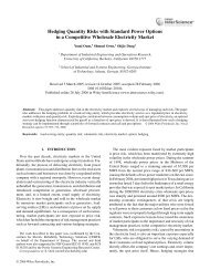
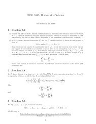
we let a cost unit be 1 cent, and a flow unit be 1 chair. To construct the associated graph <strong>for</strong><br />
the problem, we first consider the wood sources and the plants, denoted by nodes W S1, W S2 and<br />
P 1, . . . , P 4 respectively, in Figure 1a. Because each wood source can supply wood to each plant,<br />
there is an arc from each source to each plant. To reflect the transportation cost of wood from<br />
wood source to plant, the arc will have cost, along with capacity lower bound (zero) and upper<br />
bound (infinity). Arc (W S2, P 4) in Figure 1a is labeled in this manner.<br />
P1<br />
P1’<br />
P1’<br />
NY<br />
WS1<br />
P2<br />
P2’<br />
S<br />
(800, inf, 150) WS2<br />
P3<br />
P3’<br />
(800, inf, 0)<br />
wood source (0, inf, 40) P4<br />
P4’<br />
(0, inf, 190)<br />
(250, 250, 400)<br />
plant<br />
plant’<br />
(a) wood source & plants<br />
P2’<br />
Au<br />
D<br />
P3’<br />
SF<br />
(500, 1500, -1800)<br />
P4’<br />
Ch (500, 1500, 0)<br />
(0, 250, 400)<br />
(0, 250, -1400)<br />
plant’ city<br />
(b) plants & cities<br />
Figure 1: Chair Example of MCNF<br />
It is not clear exactly how much wood each wood source should supply, although we know that<br />
contract specifies that each source must supply at least 800 chairs worth of wood (or 8 tons). We<br />
represent this specification by node splitting: we create an extra node S, with an arc connecting<br />
to each wood source with capacity lower bound of 800. Cost of the arc reflects the cost of wood<br />
at each wood source. Arc (S, W S2) is labeled in this manner. Alternatively, the cost of wood can<br />
be lumped together with the cost of transportation to each plant. This is shown as the grey color<br />
labels of the arcs in the figure.<br />
Each plant has a production maximum, production minimum and production cost per unit.<br />
Again, using the node splitting technique, we create an additional node <strong>for</strong> each plant node, and<br />
labeled the arc that connect the original plant node and the new plant node accordingly. Arc<br />
(P 4, P 4 ′ ) is labeled in this manner in the figure.<br />
Each plant can distribute chairs to each city, and so there is an arc connecting each plant to<br />
each city, as shown in Figure 1b. <strong>The</strong> capacity upper bound is the production upper bound of<br />
the plant; the cost per unit is the transportation cost from the plant to the city. Similar to the<br />
wood sources, we don’t know exactly how many chairs each city will demand, although we know<br />
there is a demand upper and lower bound. We again represent this specification using the node<br />
splitting technique; we create an extra node D and specify the demand upper bound, lower bound<br />
and selling price of each unit of each city by labeling the arc that connects the city and node D.<br />
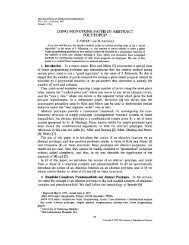
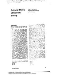
Finally, we need to relate the supply of node S to the demand of node D. <strong>The</strong>re are two ways<br />
to accomplish this. We observe that it is a closed system; there<strong>for</strong>e the number of units supplied<br />
at node S is exactly the number of units demanded at node D. So we construct an arc from node
<strong>IEOR</strong><strong>266</strong> notes: <strong>The</strong> <strong>Pseudoflow</strong> <strong>Algorithm</strong> 7<br />
P1<br />
P1’<br />
NY<br />
(0, inf, 0)<br />
S<br />
WS1<br />
WS2<br />
wood source<br />
P2<br />
P3<br />
P4<br />
P2’<br />
P3’<br />
P4’<br />
Au<br />
SF<br />
Ch<br />
D<br />
(M)<br />
S<br />
WS1<br />
WS2<br />
P1<br />
P2<br />
P3<br />
P1’<br />
P2’<br />
P3’<br />
NY<br />
Au<br />
SF<br />
D<br />
(-M)<br />
plant<br />
plant’<br />
(0, inf, 0)<br />
city<br />
wood source<br />
P4<br />
plant<br />
P4’<br />
plant’<br />
Ch<br />
city<br />
(a) circulation arc<br />
(b) drainage arc<br />
Figure 2: Complete <strong>Graph</strong> <strong>for</strong> Chair Example<br />
D to node S, with label (0, ∞, 0), as shown in Figure 2a. <strong>The</strong> total number of chairs produced will<br />
be the number of flow units in this arc. Notice that all the nodes are now transshipment nodes —<br />
such <strong>for</strong>mulations of problems are called circulation problems.<br />
Alternatively, we can supply node S with a large supply of M units, much larger than what<br />
the system requires. We then create a drainage arc from S to D with label (0, ∞, 0), as shown in<br />
Figure 2b, so the excess amount will flow directly from S to D. If the chair production operation<br />
is a money losing business, then all M units will flow directly from S to D.<br />
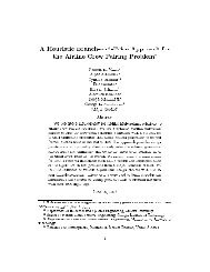
3.1 Transportation problem<br />
A problem similar to the minimum cost network flow, which is an important special case is called<br />
the transportation problem: the nodes are partitioned into suppliers and consumers only. <strong>The</strong>re<br />
are no transhippment nodes. All edges go directly from suppliers to consumers and have infinite<br />
capacity and known per unit cost. <strong>The</strong> problem is to satisfy all demands at minimum cost. <strong>The</strong><br />
assignment problem is a special case of the transportation problem, where all supply values and all<br />
demand values are 1.<br />
<strong>The</strong> graph that appears in the transportation problem is a so-called bipartite graph, or a graph<br />
in which all vertices can be divided into two classes, so that no edge connects two vertices in the<br />
same class:<br />
(V 1 ∪ V 2 ; A) ∀(u, v) ∈ A<br />
u ∈ V 1 , v ∈ V 2 (8)<br />
A property of bipartite graphs is that they are 2-colorable, that is, it is possible to assign each<br />
vertex a “color” out of a 2-element set so that no two vertices of the same color are connected.<br />
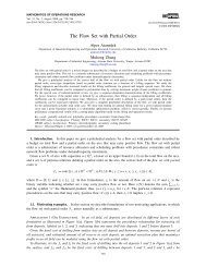
An example transportation problem is shown in Figure 3. Let s i be the supplies of nodes in V 1 ,<br />
and d j be the demands of nodes in V 2 . <strong>The</strong> transportation problem can be <strong>for</strong>mulated as an IP<br />
problem as follows:<br />
∑<br />
min<br />
i∈V 1,j∈V 2<br />
c i,j x i,j<br />
∑<br />
s.t.<br />
j∈V 2<br />
x i,j = s i ∀i ∈ V 1<br />
− ∑ i∈V 1<br />
x i,j = −d j ∀j ∈ V 2<br />
x i,j ≥ 0 x i,j integer (9)<br />
Note that assignment problem is a special case of the transportation problem. This follows from<br />
the observation that we can <strong>for</strong>mulate the assignment problem as a transportation problem with<br />
s i = d j = 1 and |V 1 | = |V 2 |.
<strong>IEOR</strong><strong>266</strong> notes: <strong>The</strong> <strong>Pseudoflow</strong> <strong>Algorithm</strong> 8<br />
(0, inf, 4)<br />
W1<br />
(-120)<br />
(180)<br />
P1<br />
W2<br />
(-100)<br />
(280)<br />
P2<br />
W3<br />
(-160)<br />
(150)<br />
P3<br />
W4<br />
(-80)<br />
plants<br />
W5<br />
(-150)<br />
warehouses<br />
Figure 3: Example of a Transportation Problem<br />
3.2 <strong>The</strong> maximum flow problem<br />
Recall the IP <strong>for</strong>mulation of the Minimum Cost Network Flow problem.<br />
( MCNF)<br />
Min cx<br />
subject to T x = b Flow balance constraints<br />
l ≤ x ≤ u, Capacity bounds<br />
Here x i,j represents the flow along the arc from i to j. We now look at some specialized variants.<br />
<strong>The</strong> Maximum Flow problem is defined on a directed network with capacities u ij on the arcs,<br />
and no costs. In addition two nodes are specified, a source node, s, and sink node, t. <strong>The</strong> objective is<br />
to find the maximum flow possible between the source and sink while satisfying the arc capacities.<br />
If x i,j represents the flow on arc (i, j), and A the set of arcs in the graph, the problem can be<br />
<strong>for</strong>mulated as:<br />
(MaxFlow)<br />
Max<br />
subject to<br />
V<br />
∑<br />
∑ (s,i)∈A x s,i = V Flow out of source<br />
∑ (j,t)∈A x j,t = V Flow in to sink<br />
(i,k)∈A x i,k − ∑ (k,j)∈A x k,j = 0, ∀k ≠ s, t<br />
l i,j ≤ x i,j ≤ u i,j , ∀(i, j) ∈ A.<br />
<strong>The</strong> Maximum Flow problem and its dual, known as the Minimum Cut problem have a number<br />
of applications and will be studied at length later in the course.<br />
3.3 <strong>The</strong> shortest path problem<br />
<strong>The</strong> Shortest Path problem is defined on a directed, weighted graph, where the weights may be<br />
thought of as distances. <strong>The</strong> objective is to find a path from a source node, s, to node a sink node,<br />
t, that minimizes the sum of weights along the path. To <strong>for</strong>mulate as a network flow problem, let<br />
x i,j be 1 if the arc (i, j) is in the path and 0 otherwise. Place a supply of one unit at s and a<br />
demand of one unit at t. <strong>The</strong> <strong>for</strong>mulation <strong>for</strong> the problem is:<br />
(SP)<br />
Min<br />
subject to<br />
∑<br />
∑((i,j)∈A d i,jx i,j<br />
∑ (i,k)∈A x i,k − ∑ (j,i)∈A x j,i = 0 ∀i ≠ s, t<br />
∑ (s,i)∈A x s,i = 1<br />
(j,t)∈A x j,t = 1<br />
0 ≤ x i,j ≤ 1
<strong>IEOR</strong><strong>266</strong> notes: <strong>The</strong> <strong>Pseudoflow</strong> <strong>Algorithm</strong> 9<br />
This problem is often solved using a variety of search and labeling algorithms depending on the<br />
structure of the graph.<br />
3.4 <strong>The</strong> single source shortest paths<br />
A related problem is the single source shortest paths problem (SSSP). <strong>The</strong> objective now is to find<br />
the shortest path from node s to all other nodes t ∈ V \ s. <strong>The</strong> <strong>for</strong>mulation is very similar, but<br />
now a flow is sent from s, which has supply n − 1, to every other node, each with demand one.<br />
(SSSP)<br />
Min<br />
subject to<br />
∑<br />
∑(i,j)∈A d i,jx i,j<br />
∑ (i,k)∈A x i,k − ∑ (j,i)∈A x j,i = −1 ∀i ≠ s<br />
(s,i)∈A x s,i = n − 1<br />
0 ≤ x i,j ≤ n − 1, ∀(i, j) ∈ A.<br />
But in this <strong>for</strong>mulation, we are minimizing the sum of all the costs to each node. How can we<br />
be sure that this is a correct <strong>for</strong>mulation <strong>for</strong> the single source shortest paths problem?<br />
<strong>The</strong>orem 3.1. For the problem of finding all shortest paths from a single node s, let ¯X be a solution<br />
and A + = {(i, j)|X ij > 0}. <strong>The</strong>n there exists an optimal solution such that the in-degree of each<br />
node j ∈ V − {s} in G = (V, A + ) is exactly 1.<br />
Proof. First, note that the in-degree of each node in V − {s} is ≥ 1, since every node has at least<br />
one path (shortest path to itself) terminating at it.<br />
If every optimal solution has the in-degree of some nodes > 1, then pick an optimal solution that<br />
minimizes ∑ j∈V −{s} indeg(j).<br />
In this solution, i.e. graph G + = (V, A + ) take a node with an in-degree > 1, say node i. Backtrack<br />
along two of the paths until you get a common node. A common node necessarily exists since both<br />
paths start from s.<br />
If one path is longer than the other, it is a contradiction since we take an optimal solution to<br />
the LP <strong>for</strong>mulation. If both paths are equal in length, we can construct an alternative solution.<br />
For a path segment, define the bottleneck link as the link in this segment that has the smallest<br />
amount of flow. And define this amount as the bottleneck amount <strong>for</strong> this path segment. Now<br />
consider the two path segments that start at a common node and end at i, and compare the<br />
bottleneck amounts <strong>for</strong> them. Pick either of the bottleneck flow. <strong>The</strong>n, move this amount of flow<br />
to the other segment, by subtracting the amount of this flow from the in-flow and out-flow of every<br />
node in this segment and adding it to the in-flow and out-flow of every node in the other segment.<br />
<strong>The</strong> cost remains the same since both segments have equal cost, but the in-degree of a node at the<br />
bottleneck link is reduced by 1 since there is no longer any flow through it.<br />
We thus have a solution where ∑ j∈V −{s}<br />
indeg(j) is reduced by 1 unit This contradiction<br />
completes the proof.<br />
<strong>The</strong> same theorem may also be proved following Linear Programming arguments by showing<br />
that a basic solution of the algorithm generated by a linear program will always be acyclic in the<br />
undirected sense.<br />
3.5 <strong>The</strong> bipartite matching problem<br />
A matching is defined as M, a subset of the edges E, such that each node is incident to at most one<br />
edge in M. Given a graph G = (V, E), find the largest cardinality matching. Maximum cardinality<br />
matching is also referred to as the Edge Packing Problem. (We know that M ≤ ⌊ V 2 ⌋.)
<strong>IEOR</strong><strong>266</strong> notes: <strong>The</strong> <strong>Pseudoflow</strong> <strong>Algorithm</strong> 10<br />
Maximum Weight Matching: We assign weights to the edges and look <strong>for</strong> maximum total<br />
weight instead of maximum cardinality. (Depending on the weights, a maximum weight matching<br />
may not be of maximum cardinality.)<br />
Smallest Cost Perfect Matching: Given a graph, find a perfect matching such that the sum of<br />
weights on the edges in the matching is minimized. On bipartite graphs, finding the smallest cost<br />
perfect matching is the assignment problem.<br />
Bipartite Matching, or Bipartite Edge-packing involves pairwise association on a bipartite graph.<br />
In a bipartite graph, G = (V, E), the set of vertices V can be partitioned into V 1 and V 2 such that<br />
all edges in E are between V 1 and V 2 . That is, no two vertices in V 1 have an edge between them, and<br />
likewise <strong>for</strong> V 2 . A matching involves choosing a collection of arcs so that no vertex is adjacent to<br />
more than one edge. A vertex is said to be “matched” if it is adjacent to an edge. <strong>The</strong> <strong>for</strong>mulation<br />
<strong>for</strong> the problem is<br />
(BM)<br />
Max<br />
subject to<br />
∑<br />
(i,j)∈E x i,j<br />
∑<br />
(i,j)∈E x i,j ≤ 1 ∀i ∈ V<br />
x i,j ∈ {0, 1}, ∀ (i, j) ∈ E.<br />
Clearly the maximum possible objective value is min{|V 1 |, |V 2 |}. If |V 1 | = |V 2 | it may be possible<br />
to have a perfect matching, that is, it may be possible to match every node.<br />
<strong>The</strong> Bipartite Matching problem can also be converted into a maximum flow problem. Add<br />
a source node, s, and a sink node t. Make all edge directed arcs from, say, V 1 to V 2 and add a<br />
directed arc of capacity 1 from s to each node in V 1 and from each node in V 2 to t. Place a supply<br />
of min{|V 1 |, |V 2 |} at s and an equivalent demand at t. Now maximize the flow from s to t. <strong>The</strong><br />
existence of a flow between two vertices corresponds to a matching. Due to the capacity constraints,<br />
no vertex in V 1 will have flow to more than one vertex in V 2 , and no vertex in V 2 will have a flow<br />
from more than one vertex in V 1 .<br />
Alternatively, one more arc from t back to s with cost of -1 can be added and the objective<br />
can be changed to maximizing circulation. Figure 4 depicts the circulation <strong>for</strong>mulation of bipartite<br />
matching problem.<br />
Figure 4: Circulation <strong>for</strong>mulation of Maximum Cardinality Bipartite Matching<br />
<strong>The</strong> problem may also be <strong>for</strong>mulated as an assignment problem. Figure 5 depicts this <strong>for</strong>mulation.<br />
An assignment problem requires that |V 1 | = |V 2 |. In order to meet this requirement we add<br />
dummy nodes to the deficient component of B as well as dummy arcs so that every node dummy<br />
or original may have its demand of 1 met. We assign costs of 0 to all original arcs and a cost of 1
<strong>IEOR</strong><strong>266</strong> notes: <strong>The</strong> <strong>Pseudoflow</strong> <strong>Algorithm</strong> 11<br />
to all dummy arcs. We then seek the assignment of least cost which will minimize the number of<br />
dummy arcs and hence maximize the number of original arcs.<br />
Figure 5: Assignment <strong>for</strong>mulation of Maximum Cardinality Bipartite Matching<br />
<strong>The</strong> General Matching, or Nonbipartite Matching problem involves maximizing the number of<br />
vertex matching in a general graph, or equivalently maximizing the size of a collection of edges<br />
such that no two edges share an endpoint. This problem cannot be converted to a flow problem,<br />
but is still solvable in polynomial time.<br />
Another related problem is the weighted matching problem in which each edge (i, j) ∈ E has<br />
weight w i,j assigned to it and the objective is to find a matching of maximum total weight. <strong>The</strong><br />
mathematical programming <strong>for</strong>mulation of this maximum weighted problem is as follows:<br />
(WM)<br />
Max<br />
subject to<br />
∑<br />
∑(i,j)∈E w i,jx i,j<br />
(i,j)∈E x i,j ≤ 1 ∀i ∈ V<br />
x i,j ∈ {0, 1}, ∀ (i, j) ∈ E.<br />
3.6 Summary of classes of network flow problems<br />
<strong>The</strong>re are a number of reasons <strong>for</strong> classifying special classes of MCNF as we have done in Figure 6.<br />
<strong>The</strong> more specialized the problem, the more efficient are the algorithms <strong>for</strong> solving it. So, it<br />
is important to identify the problem category when selecting a method <strong>for</strong> solving the problem<br />
of interest. In a similar vein, by considering problems with special structure, one may be able to<br />
design efficient special purpose algorithms to take advantage of the special structure of the problem.<br />
Note that the sets actually overlap, as Bipartite Matching is a special case of both the Assignment<br />
Problem and Max-Flow.<br />
3.7 Negative cost cycles in graphs<br />
One of the issues that can arise in weighted graphs is the existence of negative cost cycles. In this<br />
case, solving the MCNF problem gives a solution which is unbounded, there is an infinite amount<br />
of flow on the subset of the arcs comprising the negative cost cycle.<br />
This problem also occurs if we solve MCNF with upper bounds on the flow on the arcs. To see<br />
this, say we modify the <strong>for</strong>mulation with an upper bound on the flow of 1. <strong>The</strong>n, we can still have a<br />
MCNF solution that is not the shortest path, as shown in the Figure 7. In this problem the shortest<br />
path is (s, 2, 4, 3, t) while the solution to MCNF is setting the variables (x 2,4 , x 4,3 , x 3,2 , x s,1 , x 1,t ) = 1.
<strong>IEOR</strong><strong>266</strong> notes: <strong>The</strong> <strong>Pseudoflow</strong> <strong>Algorithm</strong> 12<br />
Max-Flow<br />
(No Costs)<br />
Transshipment (No capacities)<br />
✬MCNF<br />
Bipartite-Matching<br />
Transportation<br />
✩<br />
✬<br />
❄<br />
✩<br />
✬<br />
✬<br />
❄<br />
✬<br />
✩<br />
❄<br />
✩<br />
✩<br />
✬<br />
❄<br />
✩<br />
✬<br />
★<br />
✩<br />
✥<br />
✫ ✪<br />
✫<br />
✪<br />
✧<br />
✻<br />
✦<br />
✫<br />
✪<br />
✫<br />
✪ ✒<br />
✡ ✡✡✣<br />
✫<br />
✪<br />
✫<br />
✪<br />
✡ ✡✡<br />
✫<br />
✪<br />
✡ ✡✡✡<br />
✡ ✡✡ Weighted Bipartite-Matching<br />
Shortest Paths<br />
Assignment<br />
Figure 6: Classification of MCNF problems<br />
<strong>The</strong>se solutions are clearly different, meaning that solving the MCNF problem is not equivalent to<br />
solving the shortest path problem <strong>for</strong> a graph with negative cost cycles.<br />
We will study algorithms <strong>for</strong> detecting negative cost cycles in a graph later on in the course.<br />
4 Other network problems<br />
4.1 Eulerian tour<br />
We first mention the classcal Königsberg bridge problem. This problem was known at the time<br />
of Euler, who solved it in 1736 by posing it as a graph problem. <strong>The</strong> graph problem is, given an<br />
undirected graph, is there a path that traverses all edges exactly once and returns to the starting<br />
point. A graph where there exists such path is called an Eulerian graph. (You will have an<br />
opportunity to show in your homework assignment that a graph is Eulerian if and only if all node<br />
degrees are even.)<br />
Arbitrarily select edges <strong>for</strong>ming a trail until the trail closes at the starting vertex. If there are<br />
unused edges, go to a vertex that has an unused edge which is on the trail already <strong>for</strong>med, then<br />
create a “detour” - select unused edges <strong>for</strong>ming a new trail until this closes at the vertex you started
<strong>IEOR</strong><strong>266</strong> notes: <strong>The</strong> <strong>Pseudoflow</strong> <strong>Algorithm</strong> 13<br />
s<br />
1<br />
4<br />
-8 0<br />
2<br />
0<br />
3<br />
0<br />
t<br />
0<br />
1<br />
0<br />
Figure 7: Example of problem with Negative Cost Cycle<br />
with. Expand the original trail by following it to the detour vertex, then follow the detour, then<br />
continue with the original trail. If more unused edges are present, repeat this detour construction.<br />
For this algorithm we will use the adjacency list representation of a graph, the adjacency lists<br />
will be implemented using pointers. That is, <strong>for</strong> each node i in G, we will have a list of neighbors<br />
of i. In these lists each neighbor points to the next neighbor in the list and the last neighbor points<br />
to a special character to indicated that it is the last neighbor of i:<br />
n(i) = (i 1 i 2 · · · i k ⊸)<br />
d i = |{n(i)}|<br />
We will maintain a set of positive degree nodes V + . We also have an ordered list T our, and a<br />
tour pointer p T that tells us where to insert the edges that we will be adding to out tour. (In the<br />
following pseudocode we will abuse notation and let n(v) refer to the adjacency list of v and also<br />
to the first neighbor in the adjacency list of v.)<br />
Pseudocode:<br />
v ← 0 (“initial” node in the tour)<br />
T our ← (0, 0)<br />
p T initially indicates that we should insert nodes be<strong>for</strong>e the second zero.<br />
While V + ≠ ∅ do<br />
Remove edge (v, n(v)) from lists n(v) and n(n(v))<br />
d v ← d v − 1<br />
If d v = 0 then V + ← V + \ v<br />
Add n(v) to T our, and move p T to its right<br />
If V + = ∅ done<br />
If d v > 0 then<br />
v ← n(v)<br />
else<br />
find u ∈ T our ∩ V + (with d u > 0)<br />
set p T to point to the right of u (that is we must insert nodes right after u)<br />
v ← u<br />
end if<br />
end while
<strong>IEOR</strong><strong>266</strong> notes: <strong>The</strong> <strong>Pseudoflow</strong> <strong>Algorithm</strong> 14<br />
4.1.1 Eulerian walk<br />
An Eulerian walk is a path that traverses all edges exactly once (without the restriction of having<br />
to end in the starting node). It can be shown that a graph has an Eulerian path if and only if there<br />
are exactly 2 nodes of odd degree.<br />
4.2 Chinese postman problem<br />
<strong>The</strong> Chinese Postman Problem is closely related to the Eulerian walk problem.<br />
4.2.1 Undirected chinese postman problem<br />
Optimization Version: Given a graph G = (V, E) with weighted edges, traverse all edges at least<br />
once, so that the total distance traversed is minimized.<br />
This can be solved by first, identifying the odd degree nodes of the graph and constructing a<br />
complete graph with these nodes and the shortest path between them as the edges. <strong>The</strong>n if we can<br />
find a minimum weight perfect matching of this new graph, we can decide which edges to traverse<br />
twice on the Chinese postman problem and the problem reduces to finding an Eulerian walk.<br />
Decision Version: Given an edge-weighted graph G = (V, E), is there a tour traversing each edge<br />
at least once of total weight ≤ M?<br />
For edge weights = 1, the decision problem with M = |E| = m is precisely the Eulerian Tour<br />
problem. It will provide an answer to the question: Is this graph Eulerian?<br />
4.2.2 Directed chinese postman problem<br />
Given a gdirected graph G = (V, A) with weighted arcs, traverse all arcs at least once, so that the<br />
total distance traversed is minimized.<br />
Note that the necessary and sufficient condition of the existence of a directed Eulerian tour<br />
is that the indegree must equal the outdegee on every node. So this can be <strong>for</strong>mulated as a<br />
transportation problem as follows.<br />
For each odd degree node, calculate outdegree-indegree and this number will be the demand of<br />
each node. <strong>The</strong>n define the arcs by finding the shortest path from each negative demand node to<br />
each positive demand node.<br />
4.2.3 Mixed chinese postman problem<br />
Chinese Postman Problem with both directed and undirected edges. Surprisingly, this problem is<br />
intractable.<br />
4.3 Hamiltonian tour problem<br />
Given a graph G = (V, E), is there a tour visiting each node exactly once?<br />
This is a NP-complete decision problem and no polynomial algorithm is known to determine<br />
whether a graph is Hamiltonian.<br />
4.4 Traveling salesman problem (TSP)<br />
Optimization Version: Given a graph G = (V, E) with weights on the edges, visit each node<br />
exactly once along a tour, such that we minimize the total traversed weight.
<strong>IEOR</strong><strong>266</strong> notes: <strong>The</strong> <strong>Pseudoflow</strong> <strong>Algorithm</strong> 15<br />
Decision version: Given a graph G = (V, E) with weights on the edges, and a number M, is<br />
there a tour traversing each node exactly once of total weight ≤ M?<br />
4.5 Vertex packing problems (Independent Set)<br />
Given a graph G = (V, E), find a subset S of nodes such that no two nodes in the subset are<br />
neighbors, and such that S is of maximum cardinality. (We define neighbor nodes as two nodes<br />
with an edge between them.)<br />
We can also assign weights to the vertices and consider the weighted version of the problem.<br />
4.6 Maximum clique problem<br />
A “Clique” is a collection of nodes S such that each node in the set is adjacent to every other node<br />
in the set. <strong>The</strong> problem is to find a clique of maximum cardinality.<br />
Recall that given G, Ḡ is the graph composed of the same nodes and exactly those edges not<br />
in G. Every possible edge is in either G or Ḡ. <strong>The</strong> maximum independent set problem on a graph<br />
G, then, is equivalent to the maximum clique problem in Ḡ.<br />
4.7 Vertex cover problem<br />
Find the smallest collection of vertices S in an undirected graph G such that every edge in the<br />
graph is incident to some vertex in S. (Every edge in G has an endpoint in S).<br />
Notation: If V is the set of all vertices in G, and S ⊂ V is a subset of the vertices, then V − S<br />
is the set of vertices in G not in S.<br />
Lemma 4.1. If S is an independent set, then V \ S is a vertex cover.<br />
Proof. Suppose V \ S is not a vertex cover. <strong>The</strong>n there exists an edge whose two endpoints are not<br />
in V \ S. <strong>The</strong>n both endpoints must be in S. But, then S cannot be an independent set! (Recall<br />
the definition of an independent set – no edge has both endpoints in the set.) So there<strong>for</strong>e, we<br />
proved the lemma by contradiction.<br />
<strong>The</strong> proof will work the other way, too:<br />
Result: S is an independent set if and only if V − S is a vertex cover.<br />
This leads to the result that the sum of a vertex cover and its corresponding independent set is<br />
a fixed number (namely |V |).<br />
Corollary 4.2. <strong>The</strong> complement of a maximal independent set is a minimal vertex cover, and vice<br />
versa.<br />
<strong>The</strong> Vertex Cover problem is exactly the complement of the Independent Set problem.<br />
A 2-Approximation <strong>Algorithm</strong> <strong>for</strong> the Vertex Cover Problem: We can use these results to<br />
construct an algorithm to find a vertex cover that is at most twice the size of an optimal vertex<br />
cover.<br />
(1) Find M, a maximum cardinality matching in the graph.<br />
(2) Let S = {u | u is an endpoint of some edge inM}.<br />
Claim 4.3. S is a feasible vertex cover.<br />
Proof. Suppose S is not a vertex cover. <strong>The</strong>n there is an edge e which is not covered (neither of<br />
its endpoints is an endpoint of an edge in M). So if we add the edge to M (M ∪ e), we will get a<br />
feasible matching of cardinality larger than M. But, this contradicts the maximum cardinality of<br />
M.
<strong>IEOR</strong><strong>266</strong> notes: <strong>The</strong> <strong>Pseudoflow</strong> <strong>Algorithm</strong> 16<br />
Claim 4.4. |S| is at most twice the cardinality of the minimum V C<br />
Proof. Let OP T = optimal minimal vertex cover. Suppose |M| > |OP T |. <strong>The</strong>n there exists an<br />
edge e ∈ M which doesn’t have an endpoint in the vertex cover. Every vertex in the V C can cover<br />
at most one edge of the matching. (If it covered two edges in the matching, then this is not a<br />
valid matching, because a match does not allow two edges adjacent to the same node.) This is a<br />
contradiction. <strong>The</strong>re<strong>for</strong>e, |M| ≤ |OP T |. Because |S| = 2|M| , the claim follows.<br />
4.8 Edge cover problem<br />
This is analogous to the Vertex cover problem. Given G = (V, E), find a subset EC ⊂ E such that<br />
every node in V is an endpoint of some edge in EC, and EC is of minimum cardinality.<br />
As is often the case, this edge problem is of polynomial complexity, even though its vertex analog<br />
is NP-hard.<br />
4.9 b-factor (b-matching) problem<br />
This is a generalization of the Matching Problem: given the graph G = (V, E), find a subset of<br />
edges such that each node is incident to at most d edges. <strong>The</strong>re<strong>for</strong>e, the Edge Packing Problem<br />
corresponds to the 1-factor Problem.<br />
4.10 <strong>Graph</strong> colorability problem<br />
Given an undirected graph G = (V, E), assign colors c(i) to node i ∈ V , such that ∀(i, j) ∈ E; c(i) ≠<br />
c(j).<br />
Example – Map coloring: Given a geographical map, assign colors to countries such that two<br />
adjacent countries don’t have the same color. A graph corresponding to the map is constructed<br />
as follows: each country corresponds to a node, and there is an edge connecting nodes of two<br />
neighboring countries. Such a graph is always planar (see definition below).<br />
Definition – Chromatic Number: <strong>The</strong> smallest number of colors necessary <strong>for</strong> a coloring is<br />
called the chromatic number of the graph.<br />
Definition – Planar <strong>Graph</strong>: Given a graph G = (V, E), if there exists a drawing of the graph<br />
in the plane such that no edges cross except at vertices, then the graph is said to be planar.<br />
<strong>The</strong>orem 4.5 (4-color <strong>The</strong>orem). It is always possible to color a planar graph using 4 colors.<br />
Proof. A computer proof exists that uses a polynomial-time algorithm (Appel and Haken (1977)).<br />
An “elegant” proof is still unavailable.<br />
Observe that each set of nodes of the same color is an independent set. (It follows that the<br />
cardinality of the maximum clique of the graph provides a lower bound to the chromatic number.) A<br />
possible graph coloring algorithm consists in finding the maximum independent set and assigning<br />
the same color to each node contained. A second independent set can then be found on the<br />
subgraph corresponding to the remaining nodes, and so on. <strong>The</strong> algorithm, however, is both<br />
inefficient (finding a maximum independent set is NP-hard) and not optimal. It is not optimal <strong>for</strong><br />
the same reason (and same type of example) that the b-matching problem is not solvable optimally<br />
by finding a sequence of maximum cardinality matchings.<br />
Note that a 2-colorable graph is bipartite. It is interesting to note that the opposite is also true,<br />
i.e., every bipartite graph is 2-colorable. (Indeed, the concept of k-colorability and the property of
<strong>IEOR</strong><strong>266</strong> notes: <strong>The</strong> <strong>Pseudoflow</strong> <strong>Algorithm</strong> 17<br />
being k-partite are equivalent.) We can show it building a 2-coloring of a bipartite graph through<br />
the following breadth-first-search based algorithm:<br />
Initialization: Set i = 1, L = {i}, c(i) = 1.<br />
General step: Repeat until L is empty:<br />
• For each previously uncolored j ∈ N(i), (a neighbor of i), assign color c(j) = c(i) + 1 (mod 2)<br />
and add j at the end of the list L. If j is previously colored and c(j) = c(i) + 1(mod 2)<br />
proceed, else stop and declare graph is not bipartite.<br />
• Remove i from L.<br />
• Set i = first node in L.<br />
Termination: <strong>Graph</strong> is bipartite.<br />
Note that if the algorithm finds any node in its neighborhood already labeled with the opposite<br />
color, then the graph is not bipartite, otherwise it is. While the above algorithm solves the 2-color<br />
problem in O(|E|), the d-color problem <strong>for</strong> d ≥ 3 is NP-hard even <strong>for</strong> planar graphs (see Garey and<br />
Johnson, page 87).<br />
4.11 Minimum spanning tree problem<br />
Definition: An undirected graph G = (V, T ) is a tree if the following three properties are satisfied:<br />
Property 1: |T | = |V | − 1.<br />
Property 2: G is connected.<br />
Property 3: G is acyclic.<br />
(Actually, it is possible to show that any two of the properties imply the third).<br />
Definition: Given an undirected graph G = (V, E) and a subset of the edges T ⊆ E such that<br />
(V, T ) is tree, then (V, T ) is called a spanning tree of G.<br />
Minimum spanning tree problem: Given an undirected graph G = (V, E), and costs c : E → R,<br />
find T ⊆ E such that (V, T ) is a tree and ∑ (i,j)∈T<br />
c(i, j) is minimum. Such a graph (V, T ) is a<br />
Minimum Spanning Tree (MST) of G.<br />
<strong>The</strong> problem of finding an MST <strong>for</strong> a graph is solvable by a “greedy” algorithm in O(|E|log|E|).<br />
A lower bound on the worst case complexity can be easily proved to be |E|, because every arc must<br />
get compared at least once. <strong>The</strong> open question is to see if there exists a linear algorithm to solve the<br />
problem (a linear time randomized algorithm has been recently devised by Klein and Tarjan, but so<br />
far no deterministic algorithm has been provided; still, there are “almost” linear time deterministic<br />
algorithms known <strong>for</strong> solving the MST problem).<br />
5 Complexity analysis<br />
5.1 Measuring quality of an algorithm<br />
<strong>Algorithm</strong>: One approach is to enumerate the solutions, and select the best one.<br />
Recall that <strong>for</strong> the assignment problem with 70 people and 70 tasks there are 70! ≈ 2 332.4<br />
solutions. <strong>The</strong> existence of an algorithm does not imply the existence of a good algorithm!<br />
To measure the complexity of a particular algorithm, we count the number of operations that<br />
are per<strong>for</strong>med as a function of the ‘input size’. <strong>The</strong> idea is to consider each elementary operation<br />
(usually defined as a set of simple arithmetic operations such as {+, −, ×, /,
<strong>IEOR</strong><strong>266</strong> notes: <strong>The</strong> <strong>Pseudoflow</strong> <strong>Algorithm</strong> 18<br />
problem. <strong>The</strong> goal is to measure the rate, ignoring constants, at which the running time grows as<br />
the size of the input grows; it is an asymptotic analysis.<br />
Traditionally, complexity analysis has been concerned with counting the number of operations<br />
that must be per<strong>for</strong>med in the worst case.<br />
Definition 5.1 (Concrete Complexity of a problem). <strong>The</strong> complexity of a problem is the complexity<br />
of the algorithm that has the lowest complexity among all algorithms that solve the problem.<br />
5.1.1 Examples<br />
Set Membership - Unsorted list: We can determine if a particular item is in a list of n items<br />
by looking at each member of the list one by one. Thus the number of comparisons needed<br />
to find a member in an unsorted list of length n is n.<br />
Problem: given a real number x, we want to know if x ∈ S.<br />
<strong>Algorithm</strong>:<br />
1. Compare x to s i<br />
2. Stop if x = s i<br />
3. else if i ← i + 1 < n goto 1 else stop x is not in S<br />
Complexity = n comparisons in the worst case. This is also the concrete complexity of<br />
this problem. Why?<br />
Set Membership - Sorted list: We can determine if a particular item is in a list of n elements<br />
via binary search. <strong>The</strong> number of comparisons needed to find a member in a sorted list of<br />
length n is proportional to log 2 n.<br />
Problem: given a real number x, we want to know if x ∈ S.<br />
<strong>Algorithm</strong>:<br />
1. Select s med = ⌊ first+last<br />
2<br />
⌋ and compare to x<br />
2. If s med = x stop<br />
3. If s med < x then S = (s med+1 , . . . , s last ) else S = (s first , . . . , s med−1 )<br />
4. If first < last goto 1 else stop<br />
Complexity: after k th iteration<br />
n<br />
≤ 2, which implies:<br />
2 k−1<br />
n<br />
2 k−1 elements remain. We are done searching <strong>for</strong> k such that<br />
log 2 n ≤ k<br />
Thus the total number of comparisons is at most log 2 n.<br />
Aside: This binary search algorithm can be used more generally to find the zero in a monotone<br />
increasing and monotone nondecreasing functions.<br />
Matrix Multiplication: <strong>The</strong> straight<strong>for</strong>ward method <strong>for</strong> multiplying two n × n matrices takes<br />
n 3 multiplications and n 2 (n − 1) additions. <strong>Algorithm</strong>s with better complexity (though not<br />
necessarily practical, see comments later in these notes) are known. Coppersmith and Winograd<br />
(1990) came up with an algorithm with complexity Cn 2.375477 where C is large. Indeed,<br />
the constant term is so large that in their paper Coppersmith and Winograd admit that their<br />
algorithm is impractical in practice.<br />
Forest Harvesting: In this problem we have a <strong>for</strong>est divided into a number of cells. For each<br />
cell we have the following in<strong>for</strong>mation: H i - benefit <strong>for</strong> the timber company to harvest, U i<br />
- benefit <strong>for</strong> the timber company not to harvest, and B ij - the border effect, which is the<br />
benefit received <strong>for</strong> harvesting exactly one of cells i or j. This produces an m by n grid. <strong>The</strong><br />
way to solve is to look at every possible combination of harvesting and not harvesting and<br />
pick the best one. This algorithm requires (2 mn ) operations.
<strong>IEOR</strong><strong>266</strong> notes: <strong>The</strong> <strong>Pseudoflow</strong> <strong>Algorithm</strong> 19<br />
An algorithm is said to be polynomial if its running time is bounded by a polynomial in the<br />
size of the input. All but the <strong>for</strong>est harvesting algorithm mentioned above are polynomial<br />
algorithms.<br />
An algorithm is said to be strongly polynomial if the running time is bounded by a polynomial<br />
in the size of the input and is independent of the numbers involved; <strong>for</strong> example, a max-flow<br />
algorithm whose running time depends upon the size of the arc capacities is not strongly<br />
polynomial, even though it may be polynomial (as in the scaling algorithm of Edmonds and<br />
Karp). <strong>The</strong> algorithms <strong>for</strong> the sorted and unsorted set membership have strongly polynomial<br />
running time. So does the greedy algorithm <strong>for</strong> solving the minimum spanning tree problem.<br />
This issue will be returned to later in the course.<br />
Sorting: We want to sort a list of n items in nondecreasing order.<br />
Input: S = {s 1 , s 2 , . . . , s n }<br />
Output: s i1 ≤ s i2 ≤ · · · ≤ s in<br />
Bubble Sort: n ′ = n<br />
While n ′ ≥ 2<br />
i = 1<br />
while i ≤ n ′ − 1<br />
If s i > s i+1 then t = s i+1 , s i+1 = s i , s i = t<br />
i = i + 1<br />
end while<br />
n ′ ← n ′ − 1<br />
end while<br />
Output {s 1 , s 2 , . . . , s n }<br />
Basically, we iterate through each item in the list and compare it with its neighbor. If the<br />
number on the left is greater than the number on the right, we swap the two. Do this <strong>for</strong> all<br />
of the numbers in the array until we reach the end. <strong>The</strong>n we repeat the process. At the end<br />
of the first pass, the last number in the newly ordered list is in the correct location. At the<br />
end of the second pass, the last and the penultimate numbers are in the correct positions.<br />
And so <strong>for</strong>th. So we only need to repeat this process a maximum of n times.<br />
<strong>The</strong> complexity complexity of this algorithm is: ∑ n<br />
k=2 (k − 1) = n(n − 1)/2 = O(n2 ).<br />
Merge sort (a recursive procedure):<br />
Sort(L n ): (this procedure returns L sort<br />
n )<br />
begin<br />
If n < 2<br />
return L sort<br />
n<br />
else<br />
partition L n into L ⌊n/2⌋ , L ⌈n/2⌉ (L n = L ⌊n/2⌋ ∪ L ⌈n/2⌉ )<br />
Call Sort(L ⌊n/2⌋ ) (to get L sort<br />
⌊n/2⌋ )<br />
Call Sort(L ⌈n/2⌉ ) (to get L sort<br />
⌈n/2⌉ )<br />
Call Merge(L sort<br />
end if<br />
end<br />
⌊n/2⌋ , Lsort ⌈n/2⌉ )<br />
Merge(L 1 ,L 2 ): (this procedure returns L sort )<br />
begin<br />
L sort ← empty − list
<strong>IEOR</strong><strong>266</strong> notes: <strong>The</strong> <strong>Pseudoflow</strong> <strong>Algorithm</strong> 20<br />
While (length(L 1 )¿0 and length(L 2 )¿0)<br />
if first(L 1 ) ≤ first(L 2 )<br />
add first(L 1 ) to end of L sort<br />
remove first(L 1 ) from L 1<br />
else<br />
add first(L 2 ) to end of L sort<br />
remove first(L 2 ) from L 2<br />
end if<br />
end while<br />
if length(L 1 ) > 0<br />
append L 1 to L sort<br />
if length(L 2 ) > 0<br />
append L 2 to L sort<br />
end if<br />
return L sort<br />
end<br />
In words, the merge sort algorithm is as follows:<br />
1. If the input sequence has fewer than two elements, return.<br />
2. Partition the input sequence into two halves.<br />
3. Sort the two subsequences using the same algorithm.<br />
4. Merge the two sorted subsequences to <strong>for</strong>m the output sequence.<br />
Analysis:<br />
Size of list Comparisons<br />
2 n/2<br />
4 3 · n/4<br />
8 7 · n/8<br />
. . . . . .<br />
n n − 1<br />
We have at most most log 2 n levels, with at most n comparisons on each. <strong>The</strong>re<strong>for</strong>e we<br />
per<strong>for</strong>m at most n log 2 n comparisons.<br />
An alternative way to find the number of comparisons is as follows. <strong>The</strong> work done in sorting<br />
a list of n elements is the work done to sort two lists of size n/2 each, and the work done to<br />
merge the two lists which is n.<br />
( n<br />
)<br />
f(n) = 2 f + n<br />
2<br />
Using f(1) = 1, we can solve the above recurrence relation, and obtain f(n) = n log 2 n.<br />
We conclude that the complexity complexity of this algorithm is: n log 2 n.<br />
5.2 Growth of functions<br />
n ⌈log n⌉ n − 1 2 n n!<br />
1 0 0 2 1<br />
3 2 2 8 6<br />
5 3 4 32 120<br />
10 4 9 1024 3628800<br />
70 7 69 2 70 ≈ 2 332<br />
We are interested in the asymptotic behavior of the running time.
<strong>IEOR</strong><strong>266</strong> notes: <strong>The</strong> <strong>Pseudoflow</strong> <strong>Algorithm</strong> 21<br />
5.3 Definitions <strong>for</strong> asymptotic comparisons of functions<br />
We define <strong>for</strong> functions f and g,<br />
f, g : Z + → [0, ∞) .<br />
1. f(n) ∈ O(g(n)) if ∃ a constant c > 0 such that f(n) ≤ cg(n), <strong>for</strong> all n sufficiently large.<br />
2. f(n) ∈ o(g(n)) if, <strong>for</strong> any constant c > 0, f(n) < cg(n), <strong>for</strong> all n sufficiently large.<br />
3. f(n) ∈ Ω(g(n)) if ∃ a constant c > 0 such that f(n) ≥ cg(n), <strong>for</strong> all n sufficiently large.<br />
4. f(n) ∈ ω(g(n)) if, <strong>for</strong> any constant c > 0, f(n) > cg(n), <strong>for</strong> all n sufficiently large.<br />
5. f(n) ∈ Θ(g(n)) if f(n) ∈ O(g(n)) and f(n) ∈ Ω(g(n)).<br />
Examples:<br />
• Bubble sort has complexity O(n 2 )<br />
• Merge sort has complexity O(n log n)<br />
• Matrix multiplication has complexity O(n 3 )<br />
5.4 Properties of asymptotic notation<br />
We mention a few properties that can be useful when analyzing the complexity of algorithms.<br />
Proposition 5.2. f(n) ∈ Ω(g(n)) if and only if g(n) ∈ O(f(n)).<br />
<strong>The</strong> next property is often used in conjunction with L’hôpital’s Rule.<br />
Proposition 5.3. Suppose that lim n→∞<br />
f(n)<br />
g(n) exists:<br />
f(n)<br />
lim<br />
n→∞ g(n)<br />
= c .<br />
<strong>The</strong>n,<br />
1. c < ∞ implies that f(n) ∈ O(g(n)).<br />
2. c > 0 implies that f(n) ∈ Ω(g(n)).<br />
3. c = 0 implies that f(n) ∈ o(g(n)).<br />
4. 0 < c < ∞ implies that f(n) ∈ Θ(g(n)).<br />
5. c = ∞ implies that f(n) ∈ ω(g(n)).<br />
An algorithm is good or polynomial-time if the complexity is O(polynomial(length of input)).<br />
This polynomial must be of fixed degree, that is, its degree must be independent of the input length.<br />
So, <strong>for</strong> example, O(n log n ) is not polynomial.<br />
5.5 Caveats of complexity analysis<br />
One should bear in mind a number of caveats concerning the use of complexity analysis.<br />
1. Ignores the size of the numbers. <strong>The</strong> model presented is a poor one when dealing with<br />
very large numbers, as each operation is given unit cost, regardless of the size of the numbers<br />
involved. But multiplying two huge numbers, <strong>for</strong> instance, may require more ef<strong>for</strong>t than<br />
multiplying two small numbers.
<strong>IEOR</strong><strong>266</strong> notes: <strong>The</strong> <strong>Pseudoflow</strong> <strong>Algorithm</strong> 22<br />
2. Is worst case. So complexity analysis does not say much about the average case. Traditionally,<br />
complexity analysis has been a pessimistic measure, concerned with worst-case behavior.<br />
<strong>The</strong> simplex method <strong>for</strong> linear programming is known to be exponential (in the worst case),<br />
while the ellipsoid algorithm is polynomial; but, <strong>for</strong> the ellipsoid method, the average case<br />
behavior and the worst case behavior are essentially the same, whereas the average case behavior<br />
of simplex is much better than it’s worst case complexity, and in practice is preferred<br />
to the ellipsoid method.<br />
Similarly, Quicksort, which has O(n 2 ) worst case complexity, is often chosen over other sorting<br />
algorithms with O(n log n) worst case complexity. This is because QuickSort has O(n log n)<br />
average case running time and, because the constants (that we ignore in the O notation)<br />
are smaller <strong>for</strong> QuickSort than <strong>for</strong> many other sorting algorithms, it is often preferred to<br />
algorithms with “better” worst-case complexity and “equivalent” average case complexity.<br />
3. Ignores constants. We are concerned with the asymptotic behavior of an algorithm. But,<br />
because we ignore constants (as mentioned in QuickSort comments above), it may be that an<br />
algorithm with better complexity only begins to per<strong>for</strong>m better <strong>for</strong> instances of inordinately<br />
large size.<br />
Indeed, this is the case <strong>for</strong> the O(n 2.375477 ) algorithm <strong>for</strong> matrix multiplication, that is<br />
“. . . wildly impractical <strong>for</strong> any conceivable applications.” 1<br />
4. O(n 100 ) is polynomial. An algorithm that is polynomial is considered to be “good”. So<br />
an algorithm with O(n 100 ) complexity is considered good even though, <strong>for</strong> reasons already<br />
alluded to, it may be completely impractical.<br />
Still, complexity analysis is in general a very useful tool in both determining the intrinsic<br />
“hardness” of a problem and measuring the quality of a particular algorithm.<br />
5.6 A sketch of the ellipsoid method<br />
We now outline the two key features of the ellipsoid method. A linear programming problem may<br />
be <strong>for</strong>mulated in one of two ways - a primal and dual representation. <strong>The</strong> first key feature combines<br />
both <strong>for</strong>mulations in a way that <strong>for</strong>ces all feasible solutions to be optimal solutions.<br />
Primal Problem:<br />
max{c T x : Ax ≤ b, x ≥ 0} (10)<br />
Dual Problem:<br />
<strong>The</strong> optimal solution satisfies:<br />
We create a new problem combining these two <strong>for</strong>mulations:<br />
min{b T y : y T A ≥ c, y ≥ 0} (11)<br />
c T x = b T y (12)<br />
Ax ≤ b<br />
x ≥ 0<br />
y T A T ≥ c<br />
y ≥ 0<br />
b T y ≤ c T x<br />
1 See Coppersmith D. and Winograd S., Matrix Multiplication via Arithmetic Progressions. Journal of Symbolic Computation,<br />
1990 Mar, V9 N3:251-280.
<strong>IEOR</strong><strong>266</strong> notes: <strong>The</strong> <strong>Pseudoflow</strong> <strong>Algorithm</strong> 23<br />
Note that by weak duality theorem b T y ≥ c T x, so with the inequality above this gives the<br />
desired eqaultiy. Every feasible solution to this problem is an optimal solution. <strong>The</strong> ellipsoid<br />
algorithm works on this feasibilty problem as follows:<br />
1. If there is a feasible solution to the problem, then there is a basic feasible solution. Any<br />
basic solution is contained in a sphere (ellipsoid) of radius n2 log L , where L is the largest<br />
subdeterminant of the augmented constraint matrix.<br />
2. Check if the center of the ellipsoid is feasible. If yes, we are done. Otherwise, find a constraint<br />
that has been violated.<br />
3. This violated constraint specifies a hyperplane through the center and a half ellipsoid that<br />
contains all the feasible solutions.<br />
4. Reduce the search space to the smallest ellipsoid that contains the feasible half ellipsoid.<br />
5. Repeat the algorithm at the center of the new ellipsoid.<br />
Obviously this algorithm is not complete. How do we know when to stop and decide that the<br />
feasible set is empty? It’s proved that the volume of the ellipsoids scales down in each iteration<br />
by a factor of about e −1/2(n+1) , where n is the number of linearly independent constraints. Also<br />
note that a basic feasible solution only lies on a grid of mesh length (L(L − 1)) −1 . Because when<br />
we write a component of a basic feasible solution as the quotient of two integers, the denominator<br />
cannot exceed L (by Cramer’s Rule). <strong>The</strong>re<strong>for</strong>e the component-wise difference of two basic feasible<br />
solutions can be no less than (L(L−1)) −1 . Given this, it can be shown that the convex hull of basic<br />
feasible solutions has volume of at least 2 −(n+2)L . While the volume of the original search space is<br />
2 × n 2 L 2 . <strong>The</strong>re<strong>for</strong>e the algorithm terminates in O(n 2 log L) iterations. <strong>The</strong> ellipsoid method is the<br />
first polynomial time algorithm <strong>for</strong> linear programming problems. However, it is not very efficient<br />
in practice.<br />
6 <strong>Graph</strong> representations<br />
<strong>The</strong>re are different ways to store a graph in a computer, and it is important to understand how<br />
each representation may affect or improve the complexity analysis of the related algorithms. <strong>The</strong><br />
differences between each representation are based on the way in<strong>for</strong>mation is stored, so <strong>for</strong> instance,<br />
one representation may have a characteristic X very handy but characteristic Y may be very operation<br />
intensive to obtain, while an alternative representation may favor readiness of characteristic<br />
Y over characteristic X.<br />
6.1 Node-arc adjacency matrix<br />
This representation is relevant since it is the natural representation of the flow balance constraints<br />
in the LP <strong>for</strong>mulation of Network Flow problems. This representation consists on a n by m matrix,<br />
so that each of its rows correspond to a node and each of its columns correspond to an arc. <strong>The</strong><br />
(i, j) th entry of the Node-arc adjacency matrix is {1,-1}, if i th node is the start-point or endpoint<br />
(respectively) of the j th edge and {0} otherwise.<br />
As mentioned in an earlier lecture, the node-arc adjacency matrix is totally unimodular.<br />
<strong>The</strong> density of a node-arc adjacency matrix is 2 n<br />
6.2 Node-node adjacency matrix<br />
This representation consists on a n by n matrix, so that each of its rows and each of its columns<br />
correspond to a node and the row-column intersections correspond to a (possible) edge. <strong>The</strong> (i, j) th
<strong>IEOR</strong><strong>266</strong> notes: <strong>The</strong> <strong>Pseudoflow</strong> <strong>Algorithm</strong> 24<br />
entry of the Node-Node Adjacency Matrix is 1, if there is an edge from the i th node to the j th node<br />
and 0 otherwise. In the case of undirected graphs it is easy to see that the Node-Node Adjacency<br />
Matrix is a symmetric matrix.<br />
<strong>The</strong> network is described by the matrix N, whose (i, j)th entry is n ij , where<br />
n ij =<br />
{ 1 if (i, j) ∈ E<br />
0, otherwise<br />
Figure 8 depicts the node-node adjacency matrices <strong>for</strong> directed and undirected graphs.<br />
N =<br />
To<br />
j<br />
From<br />
i 1<br />
N =<br />
Node i j<br />
Node<br />
i 1<br />
j<br />
1<br />
(a) node-node adjacency matrix <strong>for</strong><br />
a directed graph<br />
(b) node-node adjacency matrix <strong>for</strong><br />
an undirected graph<br />
Figure 8: Node-node adjacency matrices<br />
Note: For undirected graphs, the node-node adjacency matrix is symmetric. <strong>The</strong> density of<br />
this matrix is 2|E| <strong>for</strong> an undirected graph, and |A| , <strong>for</strong> a directed graph. If the graph is complete,<br />
|V | 2 |V | 2<br />
then |A| = |V | · |V − 1| and the matrix N is dense.<br />
Is this matrix a good representation <strong>for</strong> a breadth-first-search? (discussed in the next section).<br />
To determine whether a node is adjacent to any other nodes, n entries need to be checked <strong>for</strong> each<br />
row. For a connected graph with n nodes and m edges, n − 1 ≤ m ≤ n(n − 1)/2, and there are<br />
O(n 2 ) searches.<br />
6.3 Node-arc adjacency list<br />
Consider a tree, which is a very sparse graph with |E| = |V | − 1. If we represent an undirected tree<br />
using the matrices described above, we use a lot of memory. A more compact representation is to<br />
write each node and its associated adjacency list.<br />
This representation consists on n linked lists, each one corresponding to a node (i) and storing all<br />
the nodes (j) <strong>for</strong> which the edge (i,j) is present in the graph. <strong>The</strong> importance of this representation<br />
is that it is the most space efficient and it normally leads to the most efficient algorithms as well.<br />
Node Adjacent Nodes<br />
1 Neighbors of node 1<br />
2 Neighbors of node 2<br />
. .<br />
n Neighbors of node n<br />
Such a representation requires 2 |E| + |V | memory spaces as opposed to |E| · |V | memory spaces<br />
<strong>for</strong> the matrix representation.
<strong>IEOR</strong><strong>266</strong> notes: <strong>The</strong> <strong>Pseudoflow</strong> <strong>Algorithm</strong> 25<br />
<strong>The</strong>re are 2 entries <strong>for</strong> every edge or arc, this results in O(m + n) size of the adjacency list<br />
representation. This is the most compact representation among the three presented here. For<br />
sparse graphs it is the preferable one.<br />
6.4 Comparison of the graph representations<br />
6.4.1 Storage efficiency comparison<br />
Representation Storage Non-Zeros Density <strong>Notes</strong><br />
Node-Arc Matrix O(mn) O(2m) 2/n Inefficient<br />
Node-Node Matrix O(n 2 ) O(m) m/n 2 Efficient <strong>for</strong> Dense <strong>Graph</strong>s<br />
Node-Arc List O(m + n) 0 1 Efficient <strong>for</strong> Sparse <strong>Graph</strong>s<br />
6.4.2 Advantages and disadvantages comparison<br />
Representation Advantages Disadvantages<br />
Node-Arc Matrix Nice <strong>The</strong>oretical Properties Not efficient in practice<br />
Node-Node Matrix Existence of edge in O(1) time List neighbors in O(n) time<br />
Node-Arc List List neighbors in O(deg(i)) time Existence of edge in O(deg(i)) time<br />
7 <strong>Graph</strong> search algorithms<br />
Given a graph G = (V, A) and a source node s ∈ V , we want to check if all the nodes ∈ V can<br />
be reached by s using only the arcs ∈ A. Essentially we want the list of all nodes reachable from<br />
s and possibly also the path from s to each node. As seen on class, this set of paths must <strong>for</strong>m<br />
a tree, this follows from the correctness-proof of the LP <strong>for</strong>mulation of the single source shortest<br />
path problem.<br />
7.1 Generic search algorithm<br />
A generic search algorithm starts with the special node, and designates it as the root of a tree.<br />
<strong>The</strong> algorithm then selects other nodes that are adjacent to that node and adds them to the tree.<br />
It continues in an iterative manner until all nodes are part of the tree. We will define methods <strong>for</strong><br />
which this selection mechanism more closely.<br />
Pseudocode <strong>for</strong> a generic search algorithm<br />
L ← {}, V T ← {root}, E T ← {}<br />
<strong>for</strong> each edge (root, v)<br />
add edge (root, v) to end of L<br />
end <strong>for</strong><br />
While L ≠ ∅<br />
Remove edge (u, v) from L<br />
If v /∈ V T<br />
E T ← E T ∪ {(u, v)}<br />
V T ← V T ∪ {v}<br />
<strong>for</strong> each edge (v, w)<br />
add edge (v, w) to end of L<br />
end <strong>for</strong><br />
end if
<strong>IEOR</strong><strong>266</strong> notes: <strong>The</strong> <strong>Pseudoflow</strong> <strong>Algorithm</strong> 26<br />
end while<br />
Two basic methods that are used to define the selection mechanism (“Remove edge (u, v) from<br />
L”) are Breadth-First-Search (BFS) and Depth-First-Search (DFS).<br />
1<br />
2<br />
10<br />
5<br />
3<br />
7 8<br />
4<br />
9<br />
6<br />
Figure 9: <strong>Graph</strong> to be searched<br />
7.2 Breadth first search (BFS)<br />
Breadth-first-search employs a first-in-first-out (FIFO) strategy and is usually implemented using<br />
a queue. To obtain the pseudocode of BFS we only need to modify the pseudocode <strong>for</strong> the generic<br />
search so that when we remove the edge (u, v) from L we remove it from the start of L.<br />
In breadth-first-search, the graph is searched in an exhaustive manner; that is, all previously<br />
unscanned neighbors of a particular node are tagged and added to the end of the reachability list<br />
(L), and then the previously unscanned neighbors of the next node in the list are added, etc.<br />
<strong>The</strong> original graph, rearranged in a breadth-first-search, shows the typically short and bushy<br />
shape of a BFS tree as shown in Figure 10.<br />
1<br />
10 5 3 2<br />
Distance 1<br />
from root<br />
7 8<br />
4<br />
Distance 2<br />
from root<br />
9<br />
6<br />
Distance 3<br />
from root<br />
Figure 10: Solid edges represent the BFS tree of the example graph. <strong>The</strong> dotted edges cannot be<br />
present in a BFS tree.<br />
Note that the BFS tree is not unique and depends on the order in which the neighbors are<br />
visited. Not all edges from the original graph are represented in the tree. However, we know that<br />
the original graph cannot contain any edges that would bridge two nonconsecutive levels in the<br />
tree. By level we mean a set of nodes such that the number of edges that connect each node to the<br />
root of the tree is the same.
<strong>IEOR</strong><strong>266</strong> notes: <strong>The</strong> <strong>Pseudoflow</strong> <strong>Algorithm</strong> 27<br />
Consider any graph. Form its BFS tree. Any edge belonging to the original graph and not<br />
in the BFS can either be from level i to level i + 1; or between two nodes at the same level. For<br />
example, consider the dotted edge in Figure 10 from node 5 to node 6. If such an edge existed in<br />
the graph, then node 6 would be a child of node 5 and hence would appear at a distance of 2 from<br />
the root.<br />
Note that an edge <strong>for</strong>ms an even cycle if it is from level i to level i + 1 in the graph and an odd<br />
cycle if it is between two nodes at the same level.<br />
<strong>The</strong>orem 7.1 (BFS Property 1). <strong>The</strong> level of a node, d(v), is the distance from s to v.<br />
Proof. First, it is clear that every element reachable from s will be explored and given a d.<br />
By induction on d(v), Q remains ordered by d, and contains only elements with d equal to k<br />
and k + 1. Indeed, elements with d = k are dequeued first and add elements with d = k + 1 to<br />
Q. Only when all elements with d = k have been used do elements with d = k + 2 start being<br />
introduced. Let “stage k” be the period where elements with d = k are dequeued.<br />
<strong>The</strong>n, again by induction, at the beginning of stage k, all nodes at distance from s less than k<br />
have been enqueued, and only those, and they contain their correct value. Assume this <strong>for</strong> k. Let<br />
v be a node at distance k + 1. It cannot have been enqueued yet at the beginning of stage k, by<br />
assumption, so at that point d(v) = ∞. But there exists at least one node u at distance k that<br />
leads to u. u is in Q, and d(u) = k by assumption. <strong>The</strong> smallest such u in Q will give v its value<br />
d(v) = d(u) + 1 = k + 1. Nodes at distance more than k + 1 have no node at distance k leading to<br />
them and will not be enqueued.<br />
Corollary 7.2 (BFS Property 2). For undirected graphs ̸ ∃{i, j} : |d(i) − d(j)| > 1<br />
(i.e. neighbors must be in adjacent levels)<br />
For directed graphs ̸ ∃(i, j) : d(j) > d(i) + 1<br />
(i.e. Can’t skip levels in <strong>for</strong>ward arcs)<br />
Claim 7.3 (BFS Complexity). BFS runs in O(m + n) time.<br />
7.3 Depth first search (DFS)<br />
Depth-first-search employs a last-in-first-out (LIFO) strategy and is usually implemented using a<br />
stack. To obtain the pseudocode of BFS we only need to modify the pseudocode <strong>for</strong> the generic<br />
search so that when we remove the edge (u, v) from L we remove it from the end of L.<br />
In depth-first-search, one searches <strong>for</strong> a previously unscanned neighbor of a given node. If such<br />
a node is found, it is added to the end of the list and is scanned out from; otherwise, the original<br />
node is removed from the list, and we scan from the node now at the end of the list.<br />
<strong>The</strong> same graph, rearranged in a depth-first-search demonstrates the typically long and skinny<br />
shape of a DFS tree as shown in Figure 11.<br />
Claim 7.4 (DFS Complexity). DFS runs in O(m + n) time.<br />
7.4 Applications of BFS and DFS<br />
7.4.1 Checking if a graph is strongly connected<br />
Definition 7.5. A graph is strongly connected if we can reach all nodes ∈ V starting from any<br />
other node ∈ V .<br />
Naive <strong>Algorithm</strong>
<strong>IEOR</strong><strong>266</strong> notes: <strong>The</strong> <strong>Pseudoflow</strong> <strong>Algorithm</strong> 28<br />
1<br />
10<br />
2<br />
7<br />
9<br />
8<br />
6<br />
3<br />
4<br />
5<br />
Figure 11: DFS tree of the example graph<br />
00: SC(G)<br />
01: For every node in V do<br />
02: R
<strong>IEOR</strong><strong>266</strong> notes: <strong>The</strong> <strong>Pseudoflow</strong> <strong>Algorithm</strong> 29<br />
Although we can use also BFS to detect cycles, DFS tends to find a cycle ’faster’. This is<br />
because if the root is not part of the cycle BFS still needs to visit all of its neighbors; while DFS<br />
will move away from the root (and hopefully towards the cycle) faster. Also, if the cycle has length<br />
k then BFS needs at least to explore floor(k/2) levels.<br />
7.4.3 Checking of a graph is bipartite<br />
Definition 7.9. A graph is bipartite if V can be partitioned into two sets such that all edges/arcs<br />
in E/A have an endpoint on each of the two sets.<br />
Claim 7.10. Checking if a graph is bipartite takes O(m + n) time.<br />
Proof. We know that a graph is bipartite if and only if it does not contains a an odd cycle. So we<br />
can run BFS from an arbitrary node v, and if it contains an edge between nodes in the same level<br />
then the graph has an odd cycle, and thus it is not bipartite.<br />
8 Shortest paths<br />
8.1 Introduction<br />
Consider graph G = (V, A), with cost c ij on arc (i, j). <strong>The</strong>re are several different, but related,<br />
shortest path problems:<br />
• Shortest s − t path: Find a shortest path from s to t (single pair).<br />
• Single source shortest paths: Find shortest path from s to all nodes.<br />
• All pairs shortest paths: Find the SP between every pair of nodes.<br />
Additionally, we can also differentiate between shortest paths problems depending on the type<br />
of graph we receive as input.<br />
We will begin by considering shortest paths (or longest paths) in Directed Acyclic <strong>Graph</strong>s<br />
(DAGs).<br />
8.2 Properties of DAGs<br />
A DAG is a Directed Acyclic graph, namely, there are no directed cycles in the graph.<br />
Definition 8.1. A Topological ordering is the assignments of numbering to the nodes 1, 2, · · · , n<br />
such that all arcs go in the <strong>for</strong>ward direction:<br />
(i, j) ∈ E ⇒ i < j<br />
It should be noted that this graphs can have O(n 2 ) arcs. We can construct such graph by the<br />
following construction: Given a set of nodes, number them arbitrarily and add all arcs (i, j) where<br />
i < j.
<strong>IEOR</strong><strong>266</strong> notes: <strong>The</strong> <strong>Pseudoflow</strong> <strong>Algorithm</strong> 30<br />
8.2.1 Topological sort and directed acyclic graphs<br />
Given a directed graph (also called a digraph), G = (N, A), we wish to topologically sort the nodes<br />
of G; that is, we wish to assign labels 1, 2, . . . , |N| to the nodes so that (i, j) ∈ A ⇒ i < j.<br />
A topological sort does not exist in general, and a trivial example to show this is a graph with<br />
two nodes, with directed edges from each node to the other. It does, however, always exist <strong>for</strong><br />
acyclic graphs. To prove this, the following definition and lemma will be useful.<br />
Definition 8.2. A (graph) property, P , is hereditary if the following is true: given a graph G<br />
with property P , any subgraph of G also has property P .<br />
Some examples of hereditary properties:<br />
• Bipartiteness.<br />
• Having not directed cycles (i.e. being a DAG)<br />
Examples of not hereditary properties:<br />
• Connectivity.<br />
• Being an Eulerian graph.<br />
Lemma 8.3. In DAG, G, there always exists a node with in-degree 0. (Similarly, a DAG always<br />
has a node with out-degree 0.)<br />
Proof. Assume by contradiction that G there is no node with in-degree 0. We arbitrarily pick<br />
a node i in G, and apply a Depth-First-Search by visiting the predecessor nodes of each such<br />
node encountered. Since every node has a predecessor, when the nodes are exhausted (which must<br />
happen since there are a finite number of nodes in the graph), we will encounter a predecessor which<br />
has already been visited. This shows that there is a cycle in G, which contradicts our assumption<br />
that G is acyclic.<br />
<strong>The</strong>orem 8.4. <strong>The</strong>re exists a topological sort <strong>for</strong> a digraph G if and only if G is a DAG (i.e. G<br />
has no directed cycles).<br />
Proof.<br />
[Only if part] Suppose there exists a topological sort <strong>for</strong> G. If there exists cycle (i 1 ,...,i k ,i 1 ), then,<br />
by the definition of topological sort above, i 1 < i 2 < ... < i k < i 1 , which is impossible. Hence, if<br />
there exists a topological sort, then G has no directed cycles.<br />
[If part] In a DAG, the nodes can be topologically sorted by using the following procedure. Assigning<br />
a node with in-degree 0 the lowest remaining label (by the previous lemma, there always exists<br />
such a node). Removing that node from the graph (recall that being a DAG is hereditary), and<br />
repeat until all nodes are labeled. <strong>The</strong> correctness of this algorithm is established by induction on<br />
the label number. <strong>The</strong> pseudocode <strong>for</strong> the algorithm to find a topological sort is given below.<br />
Topological sort (pseudocode):<br />
i ← 1<br />
While V ≠ ∅<br />
Select v ∈ V with in-degree V (v) = 0<br />
label(v) ← i<br />
i ← i + 1<br />
V ← V \ {v}; A ← A \ {(v, w) ∈ A}<br />
update in-degrees of neighbors of v<br />
end while
<strong>IEOR</strong><strong>266</strong> notes: <strong>The</strong> <strong>Pseudoflow</strong> <strong>Algorithm</strong> 31<br />
Note that the topological sort resulting from this algorithm is not unique. Further note that we<br />
could have alternately taken the node with out-degree 0, assigned it the highest remaining label,<br />
removed it from the graph, and iterated on this until no nodes remain.<br />
An example of the topological order obtained <strong>for</strong> a DAG is depicted in Figure 12. <strong>The</strong> numbers<br />
in the boxes near the nodes represent a topological order.<br />
6<br />
1<br />
4<br />
2<br />
7<br />
3 4<br />
2<br />
5<br />
7<br />
6<br />
3<br />
5<br />
1<br />
Figure 12: An example of topological ordering in a DAG. Topological orders are given in boxes.<br />
Consider the complexity analysis of the algorithm. We can have a very loose analysis and say<br />
that each node is visited at most once and then its list of neighbors has to be updated (a search of<br />
O(m) in the node-arc adjacency matrix, or O(n) in the node-node adjacency matrix, or the number<br />
of neighbors in the adjacency list data structure). <strong>The</strong>n need to find among all nodes one with<br />
indegree equal to 0. This algorithm runs in O(mn) time, or if we are more careful it can be done<br />
in O(n 2 ). <strong>The</strong> second factor of n is due to the search <strong>for</strong> a indegree 0 node. To improve on this<br />
we maintain a ”bucket” or list of nodes of indegree 0. Each time a node’s indegree is updated, we<br />
check if it is 0 and if so add it to the bucket. Now to find a node of indegree 0 is done in O(1), just<br />
lookup the bucket in any order. Updating the indegrees is done in O(m) time total throughout the<br />
algorithm, as each arc is looked at once. <strong>The</strong>re<strong>for</strong>e, Topological Sort can be implemented to run in<br />
O(m) time.<br />
8.3 Properties of shortest paths<br />
<strong>The</strong> Shortest Path Problem (hence<strong>for</strong>th SP problem) on a digraph G = (V, A) involves finding the<br />
least cost path between two given nodes s, t ∈ V . Each arc (i, j) ∈ A has a weight assigned to it,<br />
and the cost of a path is defined as the sum of the weights of all arcs in the path.<br />
Proposition 8.5. If the path (s = i 1 , i 2 , . . . , i h = t) is a shortest path from node s to t, then<br />
the subpath (s = i 1 , i 2 , . . . , i k ) is a shortest path from source to node i k , ∀ k = 2, 3, . . . , h − 1.<br />
Furthermore, <strong>for</strong> all k 1 < k 2 the subpath (i k1 , i k1 +1, . . . , i k2 ) is a shortest path from node i k1 to i k2 .<br />
Proof. <strong>The</strong> properties given above can be proven by a contradiction-type argument.<br />
This property is a rephrasing of the principle of optimality (first stated by Richard Bellman in<br />
1952), that serves to justify dynamic programming algorithms.<br />
Proposition 8.6. Let the vector ⃗ d represent the shortest path distances from the source node. <strong>The</strong>n<br />
1. d(j) ≤ d(i) + c ij , ∀ (i, j) ∈ A.<br />
2. A directed path from s to k is a shortest path if and only if d(j) = d(i) + c ij , ∀ (i, j) ∈ P .
<strong>IEOR</strong><strong>266</strong> notes: <strong>The</strong> <strong>Pseudoflow</strong> <strong>Algorithm</strong> 32<br />
<strong>The</strong> property given above is useful <strong>for</strong> backtracking and identifying the tree of shortest paths.<br />
Given the distance vector ⃗ d, we call an arc eligible if d(j) = d(i) + c ij . We may find a (shortest)<br />
path from the source s to any other node by per<strong>for</strong>ming a breadth first search of eligible arcs. <strong>The</strong><br />
graph of eligible arcs looks like a tree, plus some additional arcs in the case that the shortest paths<br />
are not unique. But we can choose one shortest path <strong>for</strong> each node so that the resulting graph of<br />
all shortest paths from s <strong>for</strong>ms a tree.<br />
Aside: When solving the shortest path problem by linear programming, a basic solution is a tree.<br />
This is because a basic solution is an in independent set of columns; and a cycle is a dependent set<br />
of columns (there<strong>for</strong>e “a basic solution cannot contain cycles”).<br />
Given and undirected graph with nonnegative weights. <strong>The</strong> following analogue algorithm solves<br />
the shortest paths problem:<br />
<strong>The</strong> String Solution: Given a shortest path problem on an undirected graph with non-negative<br />
costs, imagine physically representing the vertices by small rings (labeled 1 to n), tied to<br />
other rings with string of length equaling the cost of each edge connecting the corresponding<br />
rings. That is, <strong>for</strong> each arc (i, j), connect ring i to ring j with string of length c ij .<br />
<strong>Algorithm</strong>: To find the shortest path from vertex s to all other vertices, hold ring s and let<br />
the other nodes fall under the <strong>for</strong>ce of gravity.<br />
<strong>The</strong>n, the distance, d(k), that ring k falls represents the length of the shortest path from s<br />
to k. <strong>The</strong> strings that are taut correspond to eligible arcs, so this arcs will <strong>for</strong>m the tree of<br />
shortest paths.<br />
8.4 Alternative <strong>for</strong>mulation <strong>for</strong> SP from s to t<br />
We have already seen how to model the single source shortest path problem as a Minimum Cost<br />
Network Flow problem. Here we will give an alternative mathematical programming <strong>for</strong>mulation<br />
<strong>for</strong> the SP problem.<br />
min<br />
d(t)<br />
d(j) ≤ d(i) + c ij ∀(i, j) ∈ A<br />
d(s) = 0<br />
Where the last constraint is needed as an anchor, since otherwise we would have an infinite number<br />
of solutions. To see this, observe that we can rewrite the first constraint as d(j) − d(i) ≤ c ij ; thus,<br />
given any feasible solution d, we can obtain an infinite number of feasible solutions (all with same<br />
objective value) by adding a constant to all entries of d.<br />
This alternative mathematical programming <strong>for</strong>mulation is nothing else but the dual of the<br />
minimum-cost-network-flow-like mathematical programming <strong>for</strong>mulation of the shortest path problem.<br />
8.5 Shortest paths on a directed acyclic graph (DAG)<br />
We consider the single source shortest paths problem <strong>for</strong> a directed acyclic graph G.<br />
We address the problem of finding the SP between nodes i and j, such that i < j, assuming<br />
the graph is topologically ordered to start with. It is beneficial to sort the graph in advance, since
<strong>IEOR</strong><strong>266</strong> notes: <strong>The</strong> <strong>Pseudoflow</strong> <strong>Algorithm</strong> 33<br />
we can trivially determine that there is no path between i and j if i > j; in other words, we know<br />
that the only way to each node j is by using nodes with label less than j. <strong>The</strong>re<strong>for</strong>e, without loss<br />
of generality, we can assume that the source is labeled 1, since any node with a smaller label than<br />
the source is unreachable from the source and can thereby be removed.<br />
Given a topological sorting of the nodes, with node 1 the source, the shortest path distances<br />
can be found by using the recurrence,<br />
d(j) =<br />
min<br />
(i,j)∈A<br />
1≤i
<strong>IEOR</strong><strong>266</strong> notes: <strong>The</strong> <strong>Pseudoflow</strong> <strong>Algorithm</strong> 34<br />
7<br />
7<br />
2<br />
5<br />
1<br />
2<br />
2 0 3 0 4<br />
1<br />
5<br />
3<br />
6<br />
0<br />
7<br />
4 8<br />
0<br />
9<br />
0 10<br />
6 4<br />
11<br />
3<br />
Figure 13: Maximizing rent example<br />
See the handout titled <strong>The</strong> Equipment Replacement Problem.<br />
Lot Sizing Problem Meet the prescribed demand d j <strong>for</strong> each of the periods j = 1, 2, ..., T by<br />
producing, or carrying inventory from previous production runs. <strong>The</strong> cost of production<br />
includes fixed set up cost <strong>for</strong> producing a positive amount at any period, and a variable per<br />
unit production cost at each period. This problem can be <strong>for</strong>mulated as a shortest path<br />
problem in a DAG (AM&O page 749) if one observes that any production will be <strong>for</strong> the<br />
demand of an integer number of consecutive periods ahead. You are asked to prove this in<br />
your homework assignment.<br />
Project Management - Critical Path Method (CPM)<br />
See the handout titled Project Formulation <strong>for</strong> Designer Gene’s Relocation.<br />
This is a typical project management problem. <strong>The</strong> objective of the problem is to find the<br />
earliest time by which the project can be completed.<br />
This problem can be <strong>for</strong>mulated as a longest path problem. <strong>The</strong> reason we <strong>for</strong>mulate the<br />
problem as a longest path problem, and not as a shortest path problem (even though we want<br />
to find the earliest finish time) is that all paths in the network have to be traversed in order<br />
<strong>for</strong> the project to be completed. So the longest one will be the “bottleneck” determining the<br />
completion time of the project.<br />
We <strong>for</strong>mulate the problem as a longest path problem as follows. We create a node <strong>for</strong> each<br />
task to be per<strong>for</strong>med. We have an arc from node i to node j if activity i must precede activity<br />
j. We set the length of arc (i, j) equal to the duration of activity i. Finally we add two spacial<br />
nodes start and finish to represent the start and the finish activities (these activities with<br />
duration 0). Note that in this graph we cannot have cycles, thus we can solve the problem as<br />
a longest path problem in an acyclic network.<br />
Now we give some notation that we will use when solving this type of problems. Each node<br />
is labeled as a triplet (node name, time in node, earliest start time). Earliest start time of<br />
a node is the earliest time that work can be started on that node. Hence, the objective can<br />
also be written as the earliest start time of the finish node.<br />
<strong>The</strong>n we can solve the problem with our dynamic programming algorithm. That is, we<br />
traverse the graph in topological order and assign the label of each node according to our<br />
dynamic programming equation:<br />
t j = max<br />
(i,j) {t i + c ij )},
<strong>IEOR</strong><strong>266</strong> notes: <strong>The</strong> <strong>Pseudoflow</strong> <strong>Algorithm</strong> 35<br />
where t i is the earliest start time of activity i; and c ij is the duration of activity i.<br />
To recover the longest path, we start from node t finish , and work backwards keeping track of<br />
the preceding activity i such that t j = t i + c ij . Notice that in general more than one activity<br />
might satisfy such equation, and thus we may have several longest paths.<br />
Alternatively, we can <strong>for</strong>mulate the longest path as follows:<br />
min t finish<br />
t j ≥ t i + c ij ∀(i, j) ∈ A<br />
t start = 0<br />
From the solution of the linear program above we can identify the longest path as follows.<br />
<strong>The</strong> constraints corresponding to arcs on the longest path will be satisfied with equality.<br />
Furthermore, <strong>for</strong> each unit increase in the length of these arcs our objective value will increase<br />
also one unit. <strong>The</strong>re<strong>for</strong>e, the dual variables of these constraints will be equal to one (while<br />
all other dual variables will be equal to zero–by complementary slackness).<br />
<strong>The</strong> longest path (also known as critical path) is shown in Figure 14 with thick lines. This<br />
path is called critical because any delay in a task along this path delays the whole project<br />
path.<br />
(A,10,<br />
0)<br />
(D,8,<br />
10)<br />
(E,14,<br />
10)<br />
(L,8,<br />
28)<br />
START<br />
(B,19,<br />
0)<br />
(F,4,<br />
19)<br />
(G,1,<br />
19)<br />
(J,4,<br />
14)<br />
(K,6,<br />
23)<br />
(M,9,<br />
29)<br />
(FINISH,<br />
0,38)<br />
(H,3,<br />
19)<br />
(I,5,<br />
19)<br />
(C,13,<br />
0)<br />
(N,7,<br />
24)<br />
Binary knapsack problem<br />
Figure 14: Project management example<br />
Problem: Given a set of items, each with a weight and value (cost), determine the subset<br />
of items with maximum total weight and total cost less than a given budget.<br />
<strong>The</strong> binary knapsack problem’s mathematical programming <strong>for</strong>mulation is as follows.<br />
max<br />
n∑<br />
w j x j<br />
j=1<br />
n∑<br />
v j x j ≤ B<br />
j=1<br />
x j ∈ {0, 1}
<strong>IEOR</strong><strong>266</strong> notes: <strong>The</strong> <strong>Pseudoflow</strong> <strong>Algorithm</strong> 36<br />
<strong>The</strong> binary knapsack problem is a hard problem. However it can be solved as a longest path<br />
problem on a DAG as follows.<br />
Let f i (q) be the maximum weight achievable when considering the first i items and a budget<br />
of q, that is,<br />
f i (q) = max<br />
i∑<br />
w j x j<br />
j=1<br />
i∑<br />
v j x j ≤ q<br />
j=1<br />
x j ∈ {0, 1}<br />
Note that we are interested in finding f n (B). Additionally, note that the f i (q)’s are related<br />
with the following dynamic programming equation:<br />
f i+1 (q) = max{f i (q), f i (q − v i+1 ) + w i+1 }.<br />
<strong>The</strong> above equation can be interpreted as follows. By the principle of optimality, the maximum<br />
weight I can obtain, when considering the first i + 1 items will be achieved by either:<br />
1. Not including the i + 1 item in my selection. In which case my total weight will be equal<br />
to f i (q), i.e. equal to the maximum weight achievable with a budget of q when only<br />
considering only the first i items; or<br />
2. Including the i + 1 item in my selection. In which case my total weight will be equal to<br />
f i (q − v i+1 ) + w i+1 , i.e. equal to the maximum weight achievable when considering the<br />
first i items with a budget of q − v i+1 plus the weight of this i + 1 object.<br />
We also have the the boundary conditions:<br />
{<br />
0 0 ≤ q < v 1<br />
f 1 (q) =<br />
.<br />
w 1 B ≥ q ≥ v 1<br />
<strong>The</strong> graph associated with the knapsack problem with 4 items, w = (6, 8, 4, 5), v = (2, 3, 4, 4),<br />
and B=12 is given in Figure 15. (<strong>The</strong> figure was adapted from: Trick M., A dynamic<br />
programming approach <strong>for</strong> consistency and propagation of knapsack constraints.)<br />
Note that in general a knapsack graph will have O(nB) nodes and O(nB) edges (each node<br />
has at most two incoming arcs), it follows that we can solve the binary knapsack problem in<br />
time O(nB).<br />
remark <strong>The</strong> above running time is not polynomial in the length of the input. This is true<br />
because the number B is given using only log B bits. <strong>The</strong>re<strong>for</strong>e the size of the input <strong>for</strong> the<br />
knapsack problem is O(n log B + n log W ) (where W is the maximum w i ). Finally, since,<br />
B = 2 log B , then a running time of O(nB) is really exponential in the size of the input.<br />
8.7 Dijkstra’s algorithm<br />
Dijkstra’s algorithm is a special purpose algorithm <strong>for</strong> finding shortest paths from a single source,<br />
s, to all other nodes in a graph with non-negative edge weights.<br />
In words, Dijkstra’s algorithm assigns distance labels (from node s) to all other nodes in the<br />
graph. Node labels are either temporary or permanent. Initially all nodes have temporary labels.
<strong>IEOR</strong><strong>266</strong> notes: <strong>The</strong> <strong>Pseudoflow</strong> <strong>Algorithm</strong> 37<br />
Figure 15: <strong>Graph</strong> <strong>for</strong>mulation of a binary knapsack problem.<br />
At any iteration, a node with the least distance label is marked as permanent, and the distances<br />
to its successors are updated. This is continued until no temporary nodes are left in the graph.<br />
We give the pseudocode <strong>for</strong> Dijkstra’s algorithm below. Where P is the set of nodes with<br />
permanent labels, and T of temporarily labeled nodes.<br />
begin<br />
N + (i) := {j|(i, j) ∈ A};<br />
P := {1}; T := V \ {1};<br />
d(1) := 0 and pred(1) := 0;<br />
d(j) := c 1j and pred(j) := 1 <strong>for</strong> all j ∈ A(1),<br />
and d(j) := ∞ otherwise;<br />
while P ≠ V do<br />
begin<br />
(Node selection, also called F INDMIN)<br />
let i ∈ T be a node <strong>for</strong> which d(i) = min{d(j) : j ∈ T };<br />
P := P ∪ {i}; T := T \ {i};<br />
(Distance update)<br />
<strong>for</strong> each j ∈ N + (i) do<br />
if d(j) > d(i) + c ij then<br />
d(j) := d(i) + c ij and pred(j) := i;<br />
end<br />
end<br />
<strong>The</strong>orem 8.7 (<strong>The</strong> correctness of Dijkstra’s algorithm). Once a node joins P its label is the<br />
shortest path label.<br />
Proof. At each iteration the nodes are partitioned into subsets P and T . We will prove by induction<br />
on the size of P that the label <strong>for</strong> each node i ∈ P is the shortest distance from node 1.<br />
Base: When |P | = 1, the only node in P is s. It is correctly labeled with a distance 0.<br />
Inductive step: Assume <strong>for</strong> |P | = k and prove <strong>for</strong> |P | = k + 1.
<strong>IEOR</strong><strong>266</strong> notes: <strong>The</strong> <strong>Pseudoflow</strong> <strong>Algorithm</strong> 38<br />
Suppose that node i with d(i) = min{d(j) : j ∈ T }, was added to P , but its label d(i) is not the<br />
shortest path label. <strong>The</strong>n there should be some nodes in T along the shortest path 1 to i. Let j<br />
be the first node in T on the shortest path from 1 to i. <strong>The</strong>n the length of shortest path from 1<br />
to i = d(j) + c ji . Since d(i) is not the shortest label, d(j) + c ji < d(i), and since c ji is positive, we<br />
have d(j) < d(i). This contradicts that d(i) is the minimum of d(j) ∈ T .<br />
We next prove two invariants that are preserved during Dijkstra’s algorithm execution.<br />
Proposition 8.8. <strong>The</strong> label <strong>for</strong> each j ∈ T is the shortest distance from s such that all nodes of<br />
the path are in P (i.e. it would be the shortest path if we eliminated all arcs with both endpoints in<br />
T ).<br />
Proof. We again use induction on the size of P .<br />
Base: When |P | = 1, the only node in P is s. Also, all distance labels are initialized as follows:<br />
d(j) := c sj <strong>for</strong> all j ∈ A(1). Thus the labels are indeed the shortest distance from s, using allowing<br />
only the path (s, j).<br />
Inductive step: Assume <strong>for</strong> |P | = k and prove <strong>for</strong> |P | = k + 1.<br />
After a node i in T is labeled permanently, the distance labels in T \ {i} might decrease. After<br />
permanently labeling node i, the algorithm sets d(j) = d(i) + c ij if d(j) > d(i) + c ij , <strong>for</strong> (i, j) ∈ A.<br />
<strong>The</strong>re<strong>for</strong>e, after the distance update, by the inductive hypothesis, the path from source to j satisfies<br />
d(j) ≤ d(i) + c ij , ∀ (i, j) ∈ A s.t i ∈ P . Thus, the distance label of each node in T \ {i} is the<br />
length of the shortest path subject to the restriction that each every node in the path must belong<br />
to P ∪ {i}.<br />
Proposition 8.9. <strong>The</strong> labels of nodes joining P can only increase in successive iterations.<br />
Proof. We again use induction on the size of P .<br />
Base: When |P | = 1, the only node in P is s, which has a label 0. Since all costs are nonnegative,<br />
all other nodes will have labels ≥ 0.<br />
Inductive step: Assume <strong>for</strong> |P | = k and prove <strong>for</strong> |P | = k + 1.<br />
Assume by contradiction that node i with d(i) = min{d(j) : j ∈ T }, was added to P , but in a later<br />
iteration node j is added to P having a label d(j) < d(i). This contradicts the <strong>The</strong>orem 8.7 since<br />
if the graph had a zero-cost arc (j, i), then the shortest distance from s to i would be d(j) (< d(i)<br />
which was the label of node i when added to the permanent set).<br />
Complexity Analysis<br />
<strong>The</strong>re are two major operations in Dijkstra’s algorithm :<br />
Find minimum, which has O(n 2 ) complexity; and<br />
Update labels, which has O(m) complexity.<br />
<strong>The</strong>re<strong>for</strong>e, the complexity of Dijkstra’s algorithm is = O(n 2 + m).<br />
<strong>The</strong>re are several implementations that improve upon this running time.<br />
One improvement uses Binary Heaps: whenever a label is updated, use binary search to insert<br />
that label properly in the sorted array. This requires O(log n). <strong>The</strong>re<strong>for</strong>e, the complexity of<br />
finding the minimum label in temporary set is O(m log n), and complexity of the algorithm is<br />
O(m + m log n) = O(m log n).<br />
Another improvement is Radix Heap which has complexity O(m+n √ log C) where C = max (i,j)∈A c ij .<br />
But this is not a strongly polynomial complexity.
<strong>IEOR</strong><strong>266</strong> notes: <strong>The</strong> <strong>Pseudoflow</strong> <strong>Algorithm</strong> 39<br />
Currently, the best strongly polynomial implementation of Dijkstra’s algorithm uses Fibonacci<br />
Heaps and has complexity O(m + n log n). Since Fibonacci heaps are hard to program, this implementation<br />
is not used in practice.<br />
It is important to stress that Dijkstra’s algorithm does not work correctly in the presence of<br />
negative edge weights. In this algorithm once a node is included in the permanent set it will not be<br />
checked later again, but because of the presence of negative edge that is not correct. <strong>The</strong> problem<br />
is that the distance label of a node in the permanent set might be reduced after its inclusion in the<br />
permanent set (when considering negative cost arcs).<br />
See Figure 16 <strong>for</strong> an example such that Dijkstra’s algorithm does not work in presence of<br />
negative edge weight. Using the algorithm, we get d(3) = 3. But the actual value of d(3) is 2.<br />
✓✏<br />
1<br />
✒✑ 3 ✓✏<br />
❇<br />
❳❳❳❳❳❳3<br />
3<br />
❇ ✒✑<br />
4 ❇❇❇<br />
✒ -2<br />
✓✏ ❇◆<br />
<br />
2<br />
✒✑<br />
Figure 16: Network <strong>for</strong> which Dijkstra’s algorithm fails<br />
8.8 Bellman-Ford algorithm <strong>for</strong> single source shortest paths<br />
This algorithm can be used with networks that contain negative weighted edges. <strong>The</strong>re<strong>for</strong>e it detects<br />
the existence of negative cycles. In words, the algorithm consists of n pulses. (pulse = update<br />
of labels along all m arcs). (Hence<strong>for</strong>th we will assume that we want to find the shortest paths<br />
from node 1 to all other nodes.)<br />
Input: A (general) graph G = (V, A), and two nodes s and t.<br />
Output: <strong>The</strong> shortest path from s to t.<br />
Pseudocode<br />
Initialize : d(1) := 0, d(i) := ∞, i = 2, . . . , n<br />
For i = 1, . . . , n do<br />
P ulse : ∀ (i, j) ∈ A, d(j) := min{d(j), d(i) + C ij }<br />
To prove the algorithm’s correctness we will use the following lemma.<br />
Lemma 8.10. If there are no negative cost cycles in the network G = (N, A), then there exists a<br />
shortest path from s to any node i which uses at most n − 1 arcs.<br />
Proof. Suppose that G contains no negative cycles. Observe that at most n − 1 arcs are required<br />
to construct a path from s to any node i. Now, consider a path, P , from s to i which traverses a<br />
cycle.<br />
P = s → i 1 → i 2 → . . . → (i j → i k → . . . → i j ) → i l → . . . → i.<br />
Since G has no negative length cycles, the length of P is no less than the length of ¯P where
<strong>IEOR</strong><strong>266</strong> notes: <strong>The</strong> <strong>Pseudoflow</strong> <strong>Algorithm</strong> 40<br />
¯P = s → i 1 → i 2 → . . . → i j → i k → . . . → i l → . . . → i.<br />
Thus, we can remove all cycles from P and still retain a shortest path from s to i. Since the<br />
final path is acyclic, it must have no more than n − 1 arcs.<br />
<strong>The</strong>orem 8.11 (Invariant of the algorithm). After pulse k, all shortest paths from s of length k<br />
(in terms of number of arcs) or less have been identified.<br />
Proof. Notation : d k (j) is the label d(j) at the end of pulse k.<br />
By induction. For k = 1, obvious. Assume true <strong>for</strong> k, and prove <strong>for</strong> k + 1.<br />
Let (s, i 1 , i 2 , ..., i l , j) be a shortest path to j using k + 1 or fewer arcs.<br />
It follows that (s, i 1 , i 2 , ..., i l ) is a shortest path from s to i l using k or fewer arcs.<br />
After pulse k + 1, d k+1 (j) ≤ d k (i l ) + c il ,j.<br />
But d k (i l ) + c il ,j is the length of a shortest path from s to j using k + 1 or fewer arcs, so we<br />
know that d k+1 (j) = d k (i l ) + c il ,j.<br />
Thus, the d(˙) labels are correct after pulse k + 1.<br />
Note that the shortest paths identified in the theorem are not necessarily simple. <strong>The</strong>y may<br />
use negative cost cycles.<br />
<strong>The</strong>orem 8.12. If there exists a negative cost cycle, then there exists a node j such that d n (j) <<br />
d n−1 (j) where d k (i) is the label at iteration k.<br />
Proof. Suppose not.<br />
Let (i 1 − i 2 − ... − i k − i 1 ) be a negative cost cycle.<br />
We have d n (i j ) = d n−1 (i j ), since the labels never increase.<br />
From the optimality conditions, d n (i r+1 ) ≤ d n−1 (i r ) + C r,r+1 where r = 1,...,k-1, and d n (i 1 ) ≤<br />
d n−1 (i k ) + C ik ,i 1<br />
.<br />
<strong>The</strong>se inequalities imply ∑ k<br />
j=1 d n(i j ) ≤ ∑ k<br />
j=1 d n−1(i j ) + ∑ k<br />
j=1 C i j−1 ,i j<br />
.<br />
But if d n (i j ) = d n−1 (i j ), the above inequality implies 0 ≤ ∑ k<br />
j=1 C i j−1 ,i j<br />
.<br />
∑ k<br />
j=1 C i j−1 ,i j<br />
is the length of the cycle, so we get an inequality which says that 0 is less than a<br />
negative number which is a contradiction.<br />
Corollary 8.13. <strong>The</strong> Bellman-Ford algorithm identifies a negative cost cycle if one exists.<br />
By running n pulses of the Bellman-Ford algorithm, we either detect a negative cost cycle (if<br />
one exists) or find a shortest path from s to all other nodes i. <strong>The</strong>re<strong>for</strong>e, finding a negative cost<br />
cycle can be done in polynomial time. Interestingly, finding the most negative cost cycle is NP-hard<br />
(reduction from Hamiltonian Cycle problem).<br />
Remark Minimizing mean cost cycle is also polynomially solvable.<br />
Complexity Analysis<br />
Complexity = O(mn) since each pulse is O(m), and we have n pulses.<br />
Note that it suffices to apply the pulse operations only <strong>for</strong> arcs (i, j) where the label of i changed<br />
in the previous pulse. Thus, if no label changed in the previous iteration, then we are done.
<strong>IEOR</strong><strong>266</strong> notes: <strong>The</strong> <strong>Pseudoflow</strong> <strong>Algorithm</strong> 41<br />
8.9 Floyd-Warshall algorithm <strong>for</strong> all pairs shortest paths<br />
<strong>The</strong> Floyd-Warshall algorithm is designed to solve all pairs shortest paths problems <strong>for</strong> graphs<br />
with negative cost edges. As all algorithms <strong>for</strong> shortest paths on general graphs, this algorithm<br />
will detect negative cost cycles.<br />
In words, the algorithm maintains a matrix (d ij ) such that at iteration k, d ij is the shortest path<br />
from i to j using nodes 1, 2, ...k as intermediate nodes. After the algorithm terminates, assuming<br />
that no negative cost cycle is present, the shortest path from nodes i to j is d ij .<br />
Pseudocode<br />
Input: An n × n matrix [c ij ]<br />
Output: An n × n matrix [d ij ] is the shortest distance<br />
from i to j under [c ij ]<br />
An n × n matrix [e ij ] is a node in the path from<br />
i to j.<br />
begin<br />
<strong>for</strong> all i ≠ j do d ij := c ij ;<br />
<strong>for</strong> i = 1, . . . , n do d ii := ∞;<br />
<strong>for</strong> j = 1, . . . , n do<br />
<strong>for</strong> i = 1, . . . , n, i ≠ j, do<br />
<strong>for</strong> k = 1, . . . , n, k ≠ j, do<br />
d ik :=<br />
{<br />
min {d ik , d ij + d jk }<br />
j if d ik > d ij + d jk<br />
e ik :=<br />
e ik otherwise<br />
end<br />
<strong>The</strong> main operation in the algorithm is: P ulse j : d ik = min(d ik , d ij + d jk ). This operation is<br />
sometimes referred to as a triangle operation (see Figure 17).<br />
Figure 17: Triangle operation: Is the (dotted) path using node j as intermediate node shorter than<br />
the (solid) path without using node j?<br />
Invariant property of Floyd-Warshall <strong>Algorithm</strong>:<br />
After iteration k, d ij is the shortest path distance from i to j involving a subset of nodes in<br />
{1, 2, . . . , k} as intermediate nodes.<br />
Complexity Analysis<br />
At each iteration we consider another node as intermediate node → O(n) iterations.<br />
In each iteration we compare n 2 triangles <strong>for</strong> n 2 pairs → O(n 2 ).<br />
<strong>The</strong>re<strong>for</strong>e complexity of the Floyd-Warshall algorithm = O(n 3 ).
<strong>IEOR</strong><strong>266</strong> notes: <strong>The</strong> <strong>Pseudoflow</strong> <strong>Algorithm</strong> 42<br />
See the handout titled All pairs shortest paths.<br />
At the initial stage, d ij = c ij if there exist an arc between node i and j<br />
d ij = ∞ otherwise<br />
e ij = 0<br />
First iteration : d 24 ← min(d 24 , d 21 + d 14 ) = 3<br />
e 24 = 1<br />
Update distance label<br />
Second iteration : d 41 ← min(d 41 , d 42 + d 21 ) = −2<br />
d 43 ← min(d 43 , d 42 + d 23 ) = −3<br />
d 44 ← min(d 44 , d 42 + d 24 ) = −1<br />
e 41 = e 43 = e 44 = 2<br />
No other label changed<br />
Note that we found a negative cost cycle since the diagonal element of matrix D, d 44 = −1 ≤ 0.<br />
Negative d ii means there exists a negative cost cycle since it simply says that there exists a path<br />
of negative length from node i to itself.<br />
8.10 D.B. Johnson’s algorithm <strong>for</strong> all pairs shortest paths<br />
See the handout titled All pairs shortest paths - section 1.2.<br />
This algorithm takes advantage of the idea that if all arc costs were nonnegative, we can find<br />
all pairs shortest paths by solving O(n) single source shortest paths problems using Dijkstra’s algorithm.<br />
<strong>The</strong> algorithm converts a network with negative-cost arcs to an equivalent network with<br />
nonnegative-cost arcs. After this trans<strong>for</strong>mation, we can use Dijkstra’s algorithm to solve n SSSP<br />
(and get our APSP).<br />
D.B. Johnson’s algorithm<br />
1. Add a node s to the graph with c sj = 0 <strong>for</strong> all nodes j ∈ V .<br />
2. Use Bellman-Ford algorithm to find the shortest paths from s to every other node. If a<br />
negative cost cycle is detected by the algorithm, then terminate at this step. Otherwise, let<br />
d(i) be the shortest distance from s to node i.<br />
3. Remove s from the graph, and convert the costs in the original graph to nonnegative costs<br />
by setting c ′ ij = c ij + d(i) − d(j).<br />
4. Apply Dijkstra’s algorithm n times to the graph with weights c ′ .<br />
<strong>The</strong> correctness of the algorithm follows from the claims below.<br />
Claim 8.14. In step 1, adding node s to the graph does not create or remove negative cost cycles.<br />
Proof. Since s only has outgoing arcs, then it cannot be part of any cycle; similarly the added arcs<br />
cannot be part of any cycle. <strong>The</strong>re<strong>for</strong>e we have not created any more cycles in G. Finally, if G<br />
contained a negative cycle, this cycle remains unchanged after adding s to G.<br />
Claim 8.15. In step 3, c ′ ij ≥ 0∀(i, j) ∈ A.
<strong>IEOR</strong><strong>266</strong> notes: <strong>The</strong> <strong>Pseudoflow</strong> <strong>Algorithm</strong> 43<br />
Proof. Since d(i) are shortest path labels. <strong>The</strong>y must satisfy c ij + d(i) ≥ d(j) (Proposition 2 in<br />
<strong>Lecture</strong> 9). This implies that c ′ ij = c ij + d(i) − d(j) ≥ 0<br />
Let d P c (s, t) be the distance of a path P from s to t with the costs c.<br />
Claim 8.16. For every pair of nodes s and t, and a path P , d P c (s, t) = d P c ′ (s, t) − d(s) + d(t). That<br />
is, minimizing d c (s, t) is equivalent to minimizing d c ′(s, t).<br />
Proof. Let the path from s to t, be P = (s, i 1 , i 2 , .., i k , t).<br />
<strong>The</strong> distance along the path satisfies,<br />
d P c ′(s, t) = c si 1<br />
+ d(s) − d(i 1 ) + c si2 + d(i 1 ) − d(i 2 ) . . . + c sik + d(i k ) − d(t) = d P c (s, t) + d(s) − d(t).<br />
Note that the d(i) terms cancel out except <strong>for</strong> the first and last terms. Thus the length of all<br />
paths from s to t, when using costs c ′ instead of costs c, change by the constant amount d(s) − d(t).<br />
<strong>The</strong>re<strong>for</strong>e, the distances of path P when using c and c ′ are related as follows:<br />
d P c ′(s, t) = dP c (s, t) + d(s) − d(t).<br />
Thus, min P d P c<br />
(s, t) = min ′ P d P c (s, t)+ constant.<br />
minimizing d c (s, t).<br />
Hence minimizing d c ′(s, t) is equivalent to<br />
Complexity Analysis<br />
step 1: Add s and n arcs → O(n) step 2: Bellman-Ford → O(mn).<br />
step 3: Updating c ′ ij <strong>for</strong> m arcs → O(m).<br />
step 4: Dijkstra’s algorithm n times → O(n(m + n log n)).<br />
Total complexity: O(n(m + n log n)).<br />
So far this has been the best complexity established <strong>for</strong> the all-pairs shortest paths problem (on<br />
general graphs).<br />
8.11 Matrix multiplication algorithm <strong>for</strong> all pairs shortest paths<br />
<strong>The</strong> algorithm<br />
Consider a matrix D with d ij = c ij if there exists an arc from i to j, ∞ otherwise.<br />
Let d ii = 0 <strong>for</strong> all i. <strong>The</strong>n we define the “dot” operation as<br />
D (2)<br />
ij<br />
= (D ⊙ D T ) ij = min{d i1 + d 1j , . . . , d in + d nj }.<br />
D (2)<br />
ij<br />
represents the shortest path with 2 or fewer edges from i to j .<br />
= (D ⊙ D (2) T ) ij = shortest path with number of edges ≤ 3 from i to j<br />
D (3)<br />
ij<br />
.<br />
D (n)<br />
ij<br />
= (D ⊙ D (n−1)T ) ij = shortest path with number of edges ≤ n from i to j
<strong>IEOR</strong><strong>266</strong> notes: <strong>The</strong> <strong>Pseudoflow</strong> <strong>Algorithm</strong> 44<br />
Complexity Analysis<br />
One matrix “multiplication” (dot operation) → O(n 3 )<br />
n multiplications leads to the total complexity O(n 4 )<br />
By doubling, we can improve the complexity to O(n 3 log 2 n).<br />
of D (n)<br />
ij<br />
from its previous matrices that are powers of two.<br />
Doubling is the evaluation<br />
“Doubling”: Improving Matrix Multiplication<br />
Improving complexity by Doubling (binary powering):<br />
D (4) = D (2) ⊙ D (2)T<br />
D (8) = D (4) ⊙ D (4)T<br />
.<br />
D (2k) = D (2k−1) ⊙ D (2k−1 )T<br />
Stop once k is such that 2 k > n (i.e. need only calculate up to k = ⌈log 2 n⌉).<br />
<strong>The</strong>n, D (n) can be found by “multiplying” the appropriate matrices (based on the binary<br />
representation of n) that have been calculated via doubling. Or we can compute D (2k) , where<br />
k = ⌈log 2 n⌉ and it will be equal to D (n) since D (n) = D (n) ⊙ D T ( because the shortest path<br />
may go through at most n nodes).<br />
⇒ Complexity of algorithm with doubling is (n 3 log 2 n).<br />
Back-tracking:<br />
To find the paths, construct an ′ e ′ matrix as <strong>for</strong> Floyd-Warshall’s algorithm where e (k)<br />
ij<br />
= p if<br />
min(d (k−1)<br />
i1<br />
+ d (k−1)<br />
1j<br />
, . . . , d (k−1)<br />
in<br />
+ d (k−1)<br />
nj<br />
) = d (k−1)<br />
ip<br />
+ d (k−1)<br />
pj<br />
.<br />
p is then an intermediate node on the shortest path of length ≤ k from i to j.<br />
Identifying negative cost cycles:<br />
This is left as a question to class. Suppose there is a negative cost cycle. <strong>The</strong>n how is it<br />
detected if we only have powers of 2 computations of the matrix? <strong>The</strong> problem is to show<br />
that if there is a negative cost cycle then starting at some iteration ≤ n the distance labels<br />
of some nodes must go down at each iteration. What are these nodes?<br />
Seidel’s algorithm <strong>for</strong> Unit Cost Undirected graph:<br />
(1) Seidel has used the matrix multiplication approach <strong>for</strong> the all pairs shortest paths problem<br />
in an undirected graph. Seidel’s algorithm only works when the cost on all the arcs is 1. It<br />
uses actual matrix multiplication to find all pairs shortest paths. <strong>The</strong> running time of Seidel’s<br />
algorithm is O(M(n) log n), where M(n) is the time required to multiply two n × n matrices.<br />
(2) Currently, the most efficient (in terms of asymptotic complexity) algorithm known <strong>for</strong><br />
matrix multiplication is O(n 2.376 ). However, there is a huge constant which is hidden by the<br />
complexity notation, so the algorithm is not used in practice.<br />
8.12 Why finding shortest paths in the presence of negative cost cycles is difficult<br />
Suppose we were to apply a minimum cost flow <strong>for</strong>mulation to solve the problem of finding a<br />
shortest path from node s to node t in a graph which contains negative cost cycles. We could give<br />
a capacity of 1 to the arcs in order to guarantee a bounded solution. This is not enough, however,
<strong>IEOR</strong><strong>266</strong> notes: <strong>The</strong> <strong>Pseudoflow</strong> <strong>Algorithm</strong> 45<br />
✗✔<br />
4<br />
✖✕<br />
−10✓<br />
❙♦<br />
✓ ❙<br />
1<br />
✗✔ ✗✔ ✓✴ ✗✔ ❙<br />
1<br />
1 ✲<br />
1<br />
2 ✲ 3<br />
✖✕ ✖✕ ✖✕<br />
Figure 18: Shortest Path Problem With Negative Cost Cycles<br />
to give us a correct solution. <strong>The</strong> problem is really in ensuring that we get a simple path as a<br />
solution.<br />
Consider the network in Figure 18. Observe first that the shortest simple path from node 1 to<br />
node 2 is the arc (1, 2). If we <strong>for</strong>mulate the problem of finding a shortest path from 1 to 2 as a<br />
MCNF problem, we get the following linear program:<br />
min x 12 + x 23 + x 34 − 10x 42<br />
s.t. x 12 = 1<br />
x 23 − x 12 − x 42 = −1<br />
x 34 − x 23 = 0<br />
x 42 − x 34 = 0<br />
0 ≤ x ij ≤ 1 ∀(i, j) ∈ A.<br />
Recall that the interpretation of this <strong>for</strong>mulation is that x ij = 1 in an optimal solution means<br />
that arc (i, j) is on a shortest path from node 1 to node 2 and the path traced out by the unit of<br />
flow from node 1 to node 2 is a shortest path. In this case, however, the optimal solution to this LP<br />
is x 12 = x 23 = x 34 = x 42 = 1 which has value −7. Un<strong>for</strong>tunately, this solution does not correspond<br />
to a simple path from node 1 to node 2.<br />
9 Maximum flow problem<br />
9.1 Introduction<br />
See the handout titled Travelers Example: Seat Availability.<br />
<strong>The</strong> Maximum Flow problem is defined on a directed network G = (V, A) with capacities u ij<br />
on the arcs, and no costs. In addition two nodes are specified, a source node, s, and sink node, t.<br />
<strong>The</strong> objective is to find the maximum flow possible between the source and sink while satisfying<br />
the arc capacities. (We assume <strong>for</strong> now that all lower bounds are 0.)<br />
Definitions:<br />
• A feasible flow f is a flow that satisfied the flow-balance and capacity constraints.<br />
• A cut is a partition of the nodes (S, T ), such that S ⊆ V , s ∈ S, T = V \ S, t ∈ T .<br />
• Cut capacity: U(S, T ) = ∑ ∑<br />
i∈S j∈T u ij. (Important: note that the arcs in the cut are<br />
only those that go from S to T .)<br />
Let |f| be the total amount of flow out of the source (equivalently into the sink). It is easy to
<strong>IEOR</strong><strong>266</strong> notes: <strong>The</strong> <strong>Pseudoflow</strong> <strong>Algorithm</strong> 46<br />
observe that any feasible flow satisfies<br />
|f| ≤ U(S, T ) (13)<br />
<strong>for</strong> any (S, T ) cut. This is true since all flow goes from s to t, and since s ∈ S and t ∈ T (by<br />
definition of a cut), then all the flow must go through the arcs in the (S, T ) cut. Inequality 13 is a<br />
special case of the weak duality theorem of linear programming.<br />
<strong>The</strong> following theorem, which we will establish algorithmically, can be viewed as a special case of<br />
the strong duality theorem in linear programming.<br />
<strong>The</strong>orem 9.1 (Max-Flow Min-Cut). <strong>The</strong> value of a maximum flow is equal to the capacity of a<br />
cut with minimum capacity among all cuts. That is,<br />
max |f| = min U(S, T )<br />
Next we introduce the terminology needed to prove the Max-flow/Min-cut duality and to give<br />
us an algorithm to find the max flow of any given graph.<br />
Residual graph: <strong>The</strong> residual graph, G f = (V, A f ), with respect to a flow f, has the following<br />
arcs:<br />
• <strong>for</strong>ward arcs: (i, j) ∈ A f if (i, j) ∈ A and f ij < u ij . <strong>The</strong> residual capacity is u f ij = u ij − f ij .<br />
<strong>The</strong> residual capacity on the <strong>for</strong>ward arc tells us how much we can increase flow on the original<br />
arc (i, j) ∈ A.<br />
• reverse arcs: (j, i) ∈ A f if (i, j) ∈ A and f ij > 0. <strong>The</strong> residual capacity is u f ji = f ij. <strong>The</strong><br />
residual capacity on the reverse arc tells us how much we can decrease flow on the original<br />
arc (i, j) ∈ A.<br />
Intuitively, residual graph tells us how much additional flow can be sent through the original<br />
graph with respect to the given flow. This brings us to the notion of an augmenting path.<br />
In the presence of lower bounds, l ij ≤ f ij ≤ u ij , (i, j) ∈ A, the definition of <strong>for</strong>ward arc remains,<br />
whereas <strong>for</strong> reverse arc, (j, i) ∈ A f if (i, j) ∈ A and f ij > l ij . <strong>The</strong> residual capacity is u f ji = f ij −l ij .<br />
9.2 Linear programming duality and max flow min cut<br />
Given G = (N, A) and capacities u ij <strong>for</strong> all (i, j) ∈ A:<br />
Consider the <strong>for</strong>mulation of the maximum flow problem on a general graph. Let x ij be a variable<br />
denoting the flow on arc (i, j).<br />
Max<br />
subject to<br />
x ts<br />
∑<br />
i x ki − ∑ j x jk = 0 k ∈ V<br />
0 ≤ x ij ≤ u ij ∀(i, j) ∈ A.<br />
For dual variables we let {z ij } be the nonnegative dual variables associated with the capacity<br />
upper bounds constraints, and {λ i } the variables associated with the flow balance constraints. (I<br />
also multiply the flow balance constraints by −1, so they represent Inflow i −Outflow i = 0.)<br />
Min<br />
∑<br />
(i,j)∈A u ijz ij<br />
subject to z ij − λ i + λ j ≥ 0 ∀(i, j) ∈ A<br />
λ s − λ t ≥ 1<br />
z ij ≥ 0 ∀(i, j) ∈ A.
<strong>IEOR</strong><strong>266</strong> notes: <strong>The</strong> <strong>Pseudoflow</strong> <strong>Algorithm</strong> 47<br />
<strong>The</strong> dual problem has an infinite number of solutions: if (λ ∗ , z ∗ ) is an optimal solution, then<br />
so is (λ ∗ + C, z ∗ ) <strong>for</strong> any constant δ. To avoid that we set λ t = 0 (or to any other arbitrary value).<br />
Observe now that with this assignment there is an optimal solution with λ s = 1 and a partition of<br />
the nodes into two sets: S = {i ∈ V |λ i = 1} and ¯S = {i ∈ V |λ i = 0}.<br />
<strong>The</strong> complementary slackness condition state that the primal and dual optimal solutions x ∗ , λ ∗ , z ∗<br />
satisfy,<br />
x ∗ ij · [z ∗ ij − λ ∗ i + λ ∗ j] = 0<br />
[u ij − x ∗ ij] · z ∗ ij = 0.<br />
In an optimal solution zij ∗ − λ∗ i + λ∗ j = 0 except <strong>for</strong> the arcs in ( ¯S, S), so the first set of<br />
complementary slackness conditions provides very little in<strong>for</strong>mation on the primal variables {x ij }.<br />
Namely, that the flows are 0 on the arcs of ( ¯S, S). As <strong>for</strong> the second set, zij ∗ = 0 on all arcs other<br />
than the arcs in the cut (S, ¯S). So we can conclude that the cut arcs are saturated, but derive no<br />
further in<strong>for</strong>mation on the flow on other arcs.<br />
<strong>The</strong> only method known to date <strong>for</strong> solving the minimum cut problem requires finding a maximum<br />
flow first, and then recovering the cut partition by finding the set of nodes reachable from<br />
the source in the residual graph (or reachable from the sink in the reverse residual graph). That<br />
set is the source set of the cut, and the recovery can be done in linear time in the number of arcs,<br />
O(m).<br />
On the other hand, if we are given a minimum cut, there is no efficient way of recovering the<br />
flow values on each arc other than essentially solving from scratch. <strong>The</strong> only in<strong>for</strong>mation given<br />
by the minimum cut, is the value of the maximum flow and the fact that the arcs on the cut are<br />
saturated. Beyond that, the flows have to be calculated with the same complexity as would be<br />
required without the knowledge of the minimum cut.<br />
This asymmetry implies that it may be easier to solve the minimum cut problem than to solve<br />
the maximum flow problem. Still, no minimum cut algorithm has ever been discovered, in the sense<br />
that every so-called s, t minimum cut algorithm known, computes first the maximum flow.<br />
9.3 Applications<br />
9.3.1 Hall’s theorem<br />
Hall discovered this theorem about a necessary and sufficient condition <strong>for</strong> the existence of a perfect<br />
matching independently of the max flow min cut theorem. However the max flow min cut theorem<br />
can be used as a quick alternative proof to Hall’s theorem.<br />
<strong>The</strong>orem 9.2 (Hall). Given a bipartite graph, B = (U ∪ V, E) where |U| = |U| = n.<br />
<strong>The</strong>re is a perfect matching in B iff ∀X ⊆ U, |N(X)| ≥ |X|,<br />
where N(X) is the set of neighbors of X, N(X) ⊆ V .<br />
Proof.<br />
(⇒) If there is a perfect matching, then <strong>for</strong> every X ⊆ U the set of its neighbors N(X) contains at<br />
least all the nodes matched with X. Thus, |N(X)| ≥ |X|.<br />
(⇐) We construct a flow graph by adding: a source s, a sink t, unit-capacity arcs from s to all<br />
nodes in U, and unit-capacity arcs from all nodes in V to t. Direct all arcs in the original graph G<br />
from U to V , and set the capacity of these arcs to ∞ (See Figure 19).<br />
Assume that |N(X)| ≥ |X|, ∀ X ⊆ U. We need to show that there exists a perfect matching.<br />
Consider a finite cut (S, T ) in the flow graph defined. Let X = U ∩S. We note that N(X) ⊆ S ∩V ,<br />
else the cut is not finite.
<strong>IEOR</strong><strong>266</strong> notes: <strong>The</strong> <strong>Pseudoflow</strong> <strong>Algorithm</strong> 48<br />
U<br />
V<br />
8<br />
1<br />
1<br />
1<br />
1<br />
s<br />
1<br />
1<br />
t<br />
1<br />
.......<br />
.......<br />
1<br />
Figure 19: <strong>Graph</strong> <strong>for</strong> Hall’s <strong>The</strong>orem<br />
Since |N(X)| ≥ |X|, the capacity of the any (S, T ) cut satisfies,<br />
Now, <strong>for</strong> (S, T ) a minimum cut,<br />
U(S, T ) ≥ |N(X)| + n − |X| ≥ n.<br />
n ≤ U(S, T ) = max flow value = size of matching ≤ n.<br />
It follows that all the inequalities must be satisfied as equalities, and the matching size is n.<br />
Define, Discrepancy = − min X {|N(X)| − |X|} = max X {|X| − |N(X)|}, X ⊆ U<br />
Since U(S, T ) = n + |Γ(X)| − |X|, where X = U ∩ S,<br />
min U(S, T ) = n + min{|Γ(X)| − |X|}.<br />
Lemma 9.3. For a bipartite graph with discrepancy D, there is a matching of size n − D<br />
9.3.2 <strong>The</strong> selection problem<br />
Suppose you are going on a hiking trip. You need to decide what to take with you. Many individual<br />
items are useless unless you take something else with them. For example, taking a bottle of wine<br />
without an opener does not make too much sense. Also, if you plan to eat soup there, <strong>for</strong> example,<br />
you might want to take a set of few different items: canned soup, an opener, a spoon and a plate.<br />
<strong>The</strong> following is the <strong>for</strong>mal definition of the problem.<br />
Given a set of items J = {1, . . . , n}, a cost <strong>for</strong> each item c j , a collection of sets of items S i ⊆ J<br />
<strong>for</strong> i = 1, . . . , m, and a benefit <strong>for</strong> each set b i . We want to maximize the net benefit (= total benefit<br />
- total cost of items) selected.
<strong>IEOR</strong><strong>266</strong> notes: <strong>The</strong> <strong>Pseudoflow</strong> <strong>Algorithm</strong> 49<br />
We now give the mathematical programming <strong>for</strong>mulation:<br />
max<br />
Where,<br />
x i =<br />
y j =<br />
m∑ n∑<br />
b i x i − c j y j<br />
j=1 i=1<br />
x i ≤ y j <strong>for</strong> i = 1, . . . , m, ∀j ∈ S i<br />
x i ∈ {0, 1} <strong>for</strong> i = 1, . . . , m<br />
y j ∈ {0, 1} <strong>for</strong> j = 1, . . . , n.<br />
{ 1 if set j is selected<br />
0 otherwise<br />
{ 1 if item j is included<br />
0 otherwise<br />
We immediately recognize that the constraint matrix is totally unimodular (each row has one 1<br />
and one −1). Thus when solving the LP relaxation of the problem we will get a solution <strong>for</strong> the<br />
above IP.<br />
Nevertheless, we can do better than solving the LP. In particular we now show how the Selection<br />
Problem can be solved by finding a minimum s-t cut in an appropriate network.<br />
First we make the following observation. <strong>The</strong> optimal solution to the selection problem will<br />
consist of a collection of sets, S j , j ∈ J, and the union of their elements ( ∪ S j , j ∈ J). In particular<br />
we will never pick “extra items” since this only adds to our cost. Feasible solutions with this<br />
structure are called selections.<br />
As per the above discussion, we can limit our search to selections, and we can <strong>for</strong>mulate the<br />
selection problem as follows. Find the collection of sets S such that:<br />
max<br />
S<br />
∑<br />
b i −<br />
i∈S<br />
∑<br />
j∈ ∪ i∈S S i<br />
c j (14)<br />
<strong>The</strong> following definition will be useful in our later discussion. Given a directed graph G = (V, A),<br />
a closed set is a set C ⊆ V such that u ∈ Cand(u, v) ∈ A =⇒ v ∈ C. That is, a closed set includes<br />
all of the successors of every node in C. Note that both ∅ and V are closed sets.<br />
Now we are ready to show how we can <strong>for</strong>mulate the selection problem as a minimum cut<br />
problem. We first create a bipartite graph with sets on one side, items on the other. We add arcs<br />
from each set to all of its items. (See figure 20.) Note that a selection in this graph is represented<br />
by a collection of set nodes and all of its successors. Indeed there is a one-to-one correspondence<br />
between selections and closed sets in this graph.<br />
Next we trans<strong>for</strong>m this graph into a maxflow-mincut graph. We set the capacity of all arcs to<br />
infinity. We add a source, a sink, arcs from s to each set i with capacity b i , and arcs from from<br />
each set j to t with capacity c j . (See figure 21.)<br />
We make the following observations. <strong>The</strong>re is a one-to-one correspondence between finite cuts<br />
and selections. Indeed the source set of any finite (S, T ) cut is a selection. (If S j ∈ S then it must<br />
be true that all of its items are also in S—otherwise the cut could not be finite.) Now we are ready<br />
to state our main result.<br />
<strong>The</strong>orem 9.4. <strong>The</strong> source set of a minimum cut (S,T) is an optimal selection.
<strong>IEOR</strong><strong>266</strong> notes: <strong>The</strong> <strong>Pseudoflow</strong> <strong>Algorithm</strong> 50<br />
Figure 20: Representing selections as closed sets<br />
Figure 21: Formulation of selection problem as a min-cut problem<br />
Proof.<br />
min U(S, T ) = min ∑ b i + ∑ c j<br />
S<br />
i∈T j∈S<br />
m∑<br />
= min b i − ∑ b i + ∑<br />
i=1 i∈S j∈S<br />
= B + min − ∑ i∈S<br />
b i + ∑ j∈S<br />
c j<br />
c j<br />
= B − max ∑ i∈S<br />
b i − ∑ j∈S<br />
c j .<br />
Where B = ∑ m<br />
i=1 b i.
<strong>IEOR</strong><strong>266</strong> notes: <strong>The</strong> <strong>Pseudoflow</strong> <strong>Algorithm</strong> 51<br />
9.3.3 <strong>The</strong> maximum closure problem<br />
We begin by defining a closed set on a graph.<br />
Definition 9.5. Given a directed graph G = (V, A), a subset of the nodes D ⊂ V is closed, if <strong>for</strong><br />
every node in D, its successors are also in D.<br />
(a) Closed set<br />
(b) Not a closed set<br />
Consider a directed graph G = (V, A) where every node i ∈ V has a corresponding weight w i .<br />
<strong>The</strong> maximum closure problem is to find a closed set V ′ ⊆ V with maximum total weight. That is,<br />
the maximum closure problem is:<br />
Problem Name: Maximum closure<br />
Instance: Given a directed graph G = (V, A), and node weights (positive or negative)<br />
b i <strong>for</strong> all i ∈ V .<br />
Optimization Problem: find a closed subset of nodes V ′ ⊆ V such that ∑ i∈V ′ b i<br />
is maximum.<br />
We can <strong>for</strong>mulate the maximum closure problem as an integer linear program (ILP) as follows.<br />
max<br />
n∑<br />
w i x i<br />
i∈v<br />
s.t. x i ≤ x j ∀(i, j) ∈ A<br />
x i ∈ {0, 1} ∀i ∈ V,<br />
where x i be a binary variable that takes the value 1 if node i is in the maximum closure, and 0<br />
otherwise. <strong>The</strong> first set of constraints <strong>for</strong>ce the requirement that <strong>for</strong> every node i included in the<br />
set, its successor is also in the set. Observe that since every row has at most one 1 and one -1,<br />
the constraint matrix is totally unimodular (TUM). Specifically, this structure indicates that the<br />
problem is a dual of a flow problem.<br />
Apparently, Johnson [Jo1] seems to be the first researcher who demonstrated that the maximum<br />
closure problem is equivalent to the selection problem (max closure on bipartite graphs), and<br />
that the selection problem is solvable by max flow algorithm. Picard [Pic1], demonstrated that a<br />
minimum cut algorithm on a related graph, solves the maximum closure problem.<br />
Let V + ≡ {j ∈ V |w j > 0}, and V − ≡ {j ∈ V |w j < 0}. We construct an s, t-graph G st as<br />
follows. Given the graph G = (V, A) we set the capacity of all arcs in A equal to ∞. We add a<br />
source s, a sink t, arcs from s to all nodes i ∈ V + (with capacity u s,i = w i ), and arcs from all nodes
<strong>IEOR</strong><strong>266</strong> notes: <strong>The</strong> <strong>Pseudoflow</strong> <strong>Algorithm</strong> 52<br />
j ∈ V − to t (with capacity u j,t = |w j | = −w j ). <strong>The</strong> graph G st is a closure graph (a closure graph<br />
is a graph with a source, a sink, and with all finite capacity arcs adjacent only to either the source<br />
or the sink.) This construction is illustrated in Figure 22.<br />
Figure 22: Visual representation of G st .<br />
Claim 9.6. If (s ∪ S, t ∪ T ) is a finite s − t cut on G s,t , then S is a closed set on G.<br />
Proof. Assume by contradiction that S is not closed. This means that there must be an arc<br />
(i, j) ∈ A such that i ∈ S and j ∈ T . This arc must be on the cut (S, T ), and by construction<br />
u i,j = ∞, which is a contradiction on the cut being finite.<br />
<strong>The</strong>orem 9.7. If (s ∪ S, t ∪ T ) is an optimal solution to the minimum s − t cut problem on G s,t ,<br />
then S is a maximum closed set on G.<br />
Proof.<br />
∑<br />
∑<br />
C (s ∪ S, t ∪ T ) =<br />
u s,i +<br />
(s,i)∈A st, i∈T<br />
(j,t)∈A st, j∈S<br />
∑<br />
= w i +<br />
∑<br />
−w j<br />
i ∈ T ∩V + j ∈ S∩V −<br />
= ∑<br />
w i −<br />
∑<br />
w i −<br />
∑<br />
i∈V + i∈S∩V +<br />
u j,t<br />
j∈S∩V − w j<br />
= W + − ∑ i∈S<br />
w i<br />
(Where W + = ∑ i∈V + w i, which is a constant.) This implies that minimizing C (s ∪ S, t ∪ T ) is<br />
equivalent to minimizing W + − ∑ i∈S w i, which is in turn equivalent to<br />
max<br />
S⊆V<br />
<strong>The</strong>re<strong>for</strong>e, any source set S that minimizes the cut capacity also maximizes the sum of the weights<br />
of the nodes in S. Since by Claim 9.6 any source set of an s − t cut in G s,t is closed, we conclude<br />
that S is a maximum closed set on G.<br />
∑<br />
i∈S<br />
w i
<strong>IEOR</strong><strong>266</strong> notes: <strong>The</strong> <strong>Pseudoflow</strong> <strong>Algorithm</strong> 53<br />
Variants / Special Cases<br />
• In the minimum closure problem we seek to find a closed set with minimum total weight.<br />
This can be solved by negating the weights on the nodes in G to obtain G − , constructing G − s,t<br />
just as be<strong>for</strong>e, and solving <strong>for</strong> the maximum closure. Under this construction, the source set<br />
of a minimum s − t cut on G s,t is a minimum closed set on G. See Figure 23 <strong>for</strong> a numerical<br />
example.<br />
• <strong>The</strong> selection problem is a special case of the maximum closure problem.<br />
(a) Minimum closure problem<br />
(b) Negated graph<br />
(c) Modified (max flow) graph<br />
(d) Source of min cut = min closure set on G<br />
Figure 23: Converting a minimum closure problem to a maximum closure problem. Under this<br />
trans<strong>for</strong>mation, the source set of a minimum cut is also a minimum closed set on the original<br />
graph.<br />
Numerical Example<br />
9.3.4 <strong>The</strong> open-pit mining problem<br />
Open-pit mining is a surface mining operation in which blocks of earth are extracted from the surface<br />
to retrieve the ore contained in them. During the mining process, the surface of the land is being<br />
continuously excavated, and a deeper and deeper pit is <strong>for</strong>med until the operation terminates. <strong>The</strong>
<strong>IEOR</strong><strong>266</strong> notes: <strong>The</strong> <strong>Pseudoflow</strong> <strong>Algorithm</strong> 54<br />
final contour of this pit mine is determined be<strong>for</strong>e mining operation begins. To design the optimal<br />
pit – one that maximizes profit, the entire area is divided into blocks, and the value of the ore<br />
in each block is estimated by using geological in<strong>for</strong>mation obtained from drill cores. Each block<br />
has a weight associated with it, representing the value of the ore in it, minus the cost involved<br />
in removing the block. While trying to maximize the total weight of the blocks to be extracted,<br />
there are also contour constraints that have to be observed. <strong>The</strong>se constraints specify the slope<br />
requirements of the pit and precedence constraints that prevent blocks from being mined be<strong>for</strong>e<br />
others on top of them. Subject to these constraints, the objective is to mine the most profitable<br />
set of blocks.<br />
<strong>The</strong> problem can be represented on a directed graph G = (V, A). Each block i corresponds to a<br />
node with a weight b i representing the net value of the individual block. <strong>The</strong> net value is computed<br />
as the assessed value of the ore in that block, from which the cost of extracting that block alone<br />
is deducted. <strong>The</strong>re is a directed arc from node i to node j if block i cannot be extracted be<strong>for</strong>e<br />
block j which is on a layer right above block i. This precedence relationship is determined by the<br />
engineering slope requirements. Suppose block i cannot be extracted be<strong>for</strong>e block j, and block j<br />
cannot be extracted be<strong>for</strong>e block k. By transitivity this implies that block i cannot be extracted<br />
be<strong>for</strong>e block k. We choose in this presentation not to include the arc from i to k in the graph and<br />
the existence of a directed path from i to k implies the precedence relation. Including only arcs<br />
between immediate predecessors reduces the total number of arcs in the graph. Thus to decide<br />
which blocks to extract in order to maximize profit is equivalent to finding a maximum weight set<br />
of nodes in the graph such that all successors of all nodes are included in the set. This can be<br />
solved as the maximum closure problem in G described previously.<br />
9.3.5 Forest clearing<br />
<strong>The</strong> Forest Clearing problem is a real, practical problem. We are given a <strong>for</strong>est which needs to be<br />
selectively cut. <strong>The</strong> <strong>for</strong>est is divided into squares where every square has different kind of trees.<br />
<strong>The</strong>re<strong>for</strong>e, the value (or benefit from cutting) is different <strong>for</strong> each such square. <strong>The</strong> goal is to find<br />
the most beneficial way of cutting the <strong>for</strong>est while preserving the regulatory constraints.<br />
Version 1. One of the constraints in <strong>for</strong>est clearing is preservation of deer habitat. For example,<br />
deer like to eat in big open areas, but they like to have trees around the clearing so they can run <strong>for</strong><br />
cover if a predator comes along. If they don’t feel protected, they won’t go into the clearing to eat.<br />
So, the constraint in this version of Forest Clearing is the following: no two adjacent squares can<br />
be cut. Adjacent squares are two squares which share the same side, i.e. adjacent either vertically<br />
or horizontally.<br />
Solution. Make a grid-graph G = (V, E). For every square of <strong>for</strong>est make a node v. Assign<br />
every node v, weight w, which is equal to the amount of benefit you get when cut the corresponding<br />
square. Connect two nodes if their corresponding squares are adjacent. <strong>The</strong> resulting graph is<br />
bipartite. We can color it in a chess-board fashion in two colors, such that no two adjacent nodes<br />
are of the same color. Now, the above Forest Clearing problem is equivalent to finding a max-weight<br />
independent set in the grid-graph G. In a previous section it was shown that Maximum Independent<br />
Set Problem is equivalent to Minimum Vertex Cover Problem. <strong>The</strong>re<strong>for</strong>e, we can solve our problem<br />
by solving weighted vertex cover problem on G by finding Min-Cut in the corresponding network.<br />
This problem is solved in polynomial time.<br />
Version 2. Suppose, deer can see if the diagonal squares are cut. <strong>The</strong>n the new constraint is<br />
the following: no two adjacent vertically, horizontally or diagonally squares can be cut. We can<br />
build a grid-graph in a similar fashion as in Version 1. However, it will not be bipartite anymore,<br />
since it will have odd cycles. So, the above solution would not be applicable in this case. Moreover,
<strong>IEOR</strong><strong>266</strong> notes: <strong>The</strong> <strong>Pseudoflow</strong> <strong>Algorithm</strong> 55<br />
the problem of finding Max Weight Independent Set on such a grid-graph with diagonals is proven<br />
to be NP-complete.<br />
Another variation of Forest Clearing Problem is when the <strong>for</strong>est itself is not of a rectangular<br />
shape. Also, it might have “holes” in it, such as lakes. In this case the problem is also NP-complete.<br />
<strong>The</strong> checkered board pattern permitted to clear<br />
Because there are no odd cycles in the above grid graph of version 1, it is bipartite and the<br />
a<strong>for</strong>ementioned approach works. Nevertheless, notice that this method breaks down <strong>for</strong> graphs<br />
where cells are neighbors also if they are adjacent diagonally. An example of such a graph is given<br />
below.<br />
Such graphs are no longer bipartite. In this case, the problem has indeed been proven NP-complete<br />
in the context of producing memory chips (next application).<br />
9.3.6 Producing memory chips (VLSI layout)<br />
We are given a silicon wafer of 64K RAM VLSI chips arranged in a grid-like fashion. Some chips<br />
are damaged, those will be marked by a little dot on the top and cannot be used. <strong>The</strong> objective<br />
is to make as many 256K chips as possible out of good 64K chips. A valid 256K chip is the one<br />
where 4 little chips of 64K <strong>for</strong>m a square, (i.e. they have to be adjacent to each other in a square<br />
fashion.) Create a grid-graph G = (V, E) in the following manner: place a node in the middle of<br />
every possible 256K chip. (<strong>The</strong> adjacent 256K chips will overlap.) Similar to Version 2 of Forest<br />
Clearing Problem put an edge between every two adjacent vertically, horizontally or diagonally<br />
nodes. Now, to solve the problem we need to find a maximum independent set on G. This problem<br />
is proven to be NP-complete.
<strong>IEOR</strong><strong>266</strong> notes: <strong>The</strong> <strong>Pseudoflow</strong> <strong>Algorithm</strong> 56<br />
9.4 Flow Decomposition<br />
In many situations we would like, given a feasible flow, to know how to recreate this flow with<br />
a bunch of s − t paths. In general a feasible flow might also contain cycles. This motivates the<br />
following definition.<br />
A primitive element is either:<br />
1. A simple path P from s to t with flow δ.<br />
2. A cycle Γ with flow δ.<br />
<strong>The</strong>orem 9.8 (Flow Decomposition <strong>The</strong>orem). Any feasible flow f can be decomposed into no<br />
more than m primitive elements.<br />
Proof. <strong>The</strong> proof is by construction; that is, we will give an algorithm to find the primitive elements.<br />
Let A f = {(i, j) ∈ E : f ij > 0}, and G ′ = (V, A f ).<br />
Pseudocode<br />
While there is an arc in A f adjacent to s (i.e. while there is a positive flow from s to t), do:<br />
Begin DFS in G f from s, and stop when we either reach t along a simple path P , or<br />
found a simple cycle Γ. Let ξ denote the set of arcs of the primitive element found.<br />
Set δ = min (i,j)∈ξ {f ij }.<br />
Record either (P, δ) or (Γ, δ) as a primitive element.<br />
Update the flow in G by setting: f ij ← f ij − δ ∀(i, j) ∈ ξ.<br />
Update A f . Note that the number of arcs in A f is reduced by at least one arc.<br />
If no arc in A f leaves s, then A f must consist of cycles. While A f ≠ ∅ do:<br />
Pick any arc (i, j) ∈ A f and start DFS from i.<br />
When we come back to i (which is guaranteed by flow conservation), we found another<br />
primitive element, a cycle Γ.<br />
Set δ = min (i,j)∈Γ {f ij }.<br />
Record (Γ, δ) as a primitive element.<br />
Update the flow in G by setting: f ij ← f ij − δ ∀(i, j) ∈ ξ.<br />
Update A f . Note that the number of arcs in A f<br />
Note that the above algorithm is correct since, every time we update the flow, the new flow must<br />
still be a feasible flow.<br />
Since, each time we found a primitive element we removed at least one arc from A f , we can<br />
find at most m primitive elements.<br />
An interesting question is the complexity of the algorithm to generate the primitive elements<br />
and how it compares to maximum flow. We now show that the overall complexity is O(mn).<br />
Assuming the we have <strong>for</strong> each node the adjacency list - the outgoing arcs. Follow a path from s<br />
in a DFS manner, visiting one arc at a time. If a node is repeated (visited twice) then we found<br />
a cycle. We trace it back and find its bottleneck capacity and record the primitive element. <strong>The</strong><br />
bottleneck arcs are removed, and the adjacency lists affected are updated. This entire operation is<br />
done in O(n) as we visit at most n nodes.<br />
If a node is not repeated, then after at most n steps we reached the sink t. <strong>The</strong> path followed<br />
is then a primitive path with flow equal to its bottleneck capacity. We record it and update the<br />
flows and adjacency lists in O(n) time.<br />
Since there are O(m) primitive elements, then all are found in O(mn). Notice that this is<br />
(pretty much) faster than any known maximum flow algorithm.
<strong>IEOR</strong><strong>266</strong> notes: <strong>The</strong> <strong>Pseudoflow</strong> <strong>Algorithm</strong> 57<br />
9.5 <strong>Algorithm</strong>s<br />
First we introduce some terminology that will be useful in the presentation of the algorithms.<br />
Residual graph: <strong>The</strong> residual graph, G f = (V, A f ), with respect to a flow f, has the following<br />
arcs:<br />
• <strong>for</strong>ward arcs: (i, j) ∈ A f if (i, j) ∈ A and f ij < u ij . <strong>The</strong> residual capacity is u f ij = u ij − f ij .<br />
<strong>The</strong> residual capacity on the <strong>for</strong>ward arc tells us how much we can increase flow on the original<br />
arc (i, j) ∈ A.<br />
• reverse arcs: (j, i) ∈ A f if (i, j) ∈ A and f ij > 0. <strong>The</strong> residual capacity is u f ji = f ij. <strong>The</strong><br />
residual capacity on the reverse arc tells us how much we can decrease flow on the original<br />
arc (i, j) ∈ A.<br />
Intuitively, residual graph tells us how much additional flow can be sent through the original<br />
graph with respect to the given flow. This brings us to the notion of an augmenting path.<br />
In the presence of lower bounds, l ij ≤ f ij ≤ u ij , (i, j) ∈ A, the definition of <strong>for</strong>ward arc remains,<br />
whereas <strong>for</strong> reverse arc, (j, i) ∈ A f if (i, j) ∈ A and f ij > l ij . <strong>The</strong> residual capacity is u f ji = f ij −l ij .<br />
Augmenting path: An augmenting path is a path from s to t in the residual graph. <strong>The</strong> capacity<br />
of an augmenting path is the minimum residual capacity of the arcs on the path – the bottleneck<br />
capacity.<br />
If we can find an augmenting path with capacity δ in the residual graph, we can increase the flow<br />
in the original graph by adding δ units of flow on the arcs in the original graph which correspond<br />
to <strong>for</strong>ward arcs in the augmenting path and subtracting δ units of flow on the arcs in the original<br />
graph which correspond to reverse arcs in the augmenting path.<br />
Note that this operation does not violate the capacity constraints since δ is the smallest arc<br />
capacity in the augmenting path in the residual graph, which means that we can always add δ units<br />
of flow on the arcs in the original graph which correspond to <strong>for</strong>ward arcs in the augmenting path<br />
and subtract δ units of flow on the arcs in the original graph which correspond to reverse arcs in<br />
the augmenting path without violating capacity constraints.<br />
<strong>The</strong> flow balance constraints are not violated either, since <strong>for</strong> every node on the augmenting<br />
path in the original graph we either increment the flow by δ on one of the incoming arcs and<br />
increment the flow by δ on one of the outgoing arcs (this is the case when the incremental flow in<br />
the residual graph is along <strong>for</strong>ward arcs) or we increment the flow by δ on one of the incoming arcs<br />
and decrease the flow by δ on some other incoming arc (this is the case when the incremental flow<br />
in the residual graph comes into the node through the <strong>for</strong>ward arc and leaves the node through the<br />
reverse arc) or we decrease the flow on one of the incoming arcs and one of the outgoing arcs in the<br />
original graph (which corresponds to sending flow along the reverse arcs in the residual graph).<br />
9.5.1 Ford-Fulkerson algorithm<br />
<strong>The</strong> above discussion can be summarized in the following algorithm <strong>for</strong> finding the maximum flow<br />
on a give graph. This algorithm is is also known as the augmenting path algorithm. Below is<br />
a pseudocode-like description.<br />
Pseudocode:<br />
f: flow;<br />
G f : the residual graph with respect to the flow;<br />
P st : a path from s to t;<br />
u ij : capacity of arc from i to j.
<strong>IEOR</strong><strong>266</strong> notes: <strong>The</strong> <strong>Pseudoflow</strong> <strong>Algorithm</strong> 58<br />
Initialize f = 0<br />
If ∃P st ∈ G f do<br />
find δ = min (i,j)∈Pst U ij<br />
f ij = f ij + δ ∀(i, j) ∈ P st<br />
else stop f is max flow.<br />
Detailed description:<br />
1. Start with a feasible flow (usually f ij = 0 ∀(i, j) ∈ A ).<br />
2. Construct the residual graph G f with respect to the flow.<br />
3. Search <strong>for</strong> augmenting path by doing breadth-first-search from s (we consider nodes to be<br />
adjacent if there is a positive capacity arc between them in the residual graph) and seeing<br />
whether the set of s-reachable nodes (call it S) contains t.<br />
If S contains t then there is an augmenting path (since we get from s to t by going through a<br />
series of adjacent nodes), and we can then increment the flow along the augmenting path by<br />
the value of the smallest arc capacity of all the arcs on the augmenting path.<br />
We then update the residual graph (by setting the capacities of the <strong>for</strong>ward arcs on the<br />
augmenting path to the difference between the current capacities of the <strong>for</strong>ward arcs on the<br />
augmenting path and the value of the flow on the augmenting path and setting the capacities<br />
of the reverse arcs on the augmenting path to the sum of the current capacities and the value<br />
of the flow on the augmenting path) and go back to the beginning of step 3.<br />
If S does not contain t then the flow is maximum.<br />
To establish correctness of the augmenting path algorithm we prove the following theorem which<br />
is actually stronger than the the max-flow min-cut theorem.<br />
Reminder: f ij is the flow from i to j, |f| = ∑ (s,i)∈A f si = ∑ (i,t)∈A f it = ∑ u∈S,v∈T f uv <strong>for</strong> any<br />
cut (S, T ).<br />
<strong>The</strong>orem 9.9 (Augmenting Path <strong>The</strong>orem). (generalization of the max-flow min-cut theorem)<br />
<strong>The</strong> following conditions are equivalent:<br />
1. f is a maximum flow.<br />
2. <strong>The</strong>re is no augmenting path <strong>for</strong> f.<br />
3. |f| = U(S, T ) <strong>for</strong> some cut (S, T ).<br />
Proof.<br />
(1 ⇒ 2) If ∃ augmenting path p, then we can strictly increase the flow along p; this contradicts<br />
that the flow was maximum.<br />
(2 ⇒ 3) Let G f be the residual graph w.r.t. f. Let S be a set of nodes reachable in G f from s.<br />
Let T = V \ S. Since s ∈ S and t ∈ T then (S, T ) is a cut. For v ∈ S, w ∈ T, we have the following<br />
implications:<br />
(v, w) ∉ G f ⇒ f vw = u vw and f wv = 0<br />
⇒ |f| = ∑<br />
f vw −<br />
∑<br />
v∈S,w∈T<br />
w∈T,v∈S<br />
f wv =<br />
∑<br />
v∈S,w∈T<br />
u vw = U(S, T )<br />
(3 ⇒ 1) Since |f| ≤ U(S, T ) <strong>for</strong> any (S, T ) cut, then |f| = U(S, T ) =⇒ f is a maximum flow.<br />
Note that the equivalence of conditions 1 and 3 gives the max-flow min-cut theorem.<br />
Given the max flow (with all the flow values), a min cut can be found in by looking at the residual
<strong>IEOR</strong><strong>266</strong> notes: <strong>The</strong> <strong>Pseudoflow</strong> <strong>Algorithm</strong> 59<br />
network. <strong>The</strong> set S, consists of s and the all nodes that s can reach in the final residual network<br />
and the set ¯S consists of all the other nodes. Since s can’t reach any of the nodes in ¯S, it follows<br />
that any arc going from a node in S to a node in ¯S in the original network must be saturated which<br />
implies this is a minimum cut. This cut is known as the minimal source set minimum cut. Another<br />
way to find a minimum cut is to let ¯S be t and all the nodes that can reach t in the final residual<br />
network. This a maximal source set minimum cut which is different from the minimal source set<br />
minimum cut when the minimum cut is not unique.<br />
While finding a minimum cut given a maximum flow can be done in linear time, O(m), we have<br />
yet to discover an efficient way of finding a maximum flow given a list of the edges in a minimum cut<br />
other than simply solving the maximum flow problem from scratch. Also, we have yet to discover<br />
a way of finding a minimum cut without first finding a maximum flow. Since the minimum cut<br />
problem is asking <strong>for</strong> less in<strong>for</strong>mation than the maximum flow problem, it seems as if we should be<br />
able to solve the <strong>for</strong>mer problem more efficiently than the later one. More on this in Section 9.2.<br />
In a previous lecture we already presented Ford-Fulkerson algorithm and proved its correctness.<br />
In this section we will analyze its complexity. For completeness purposes we give a sketch of the<br />
algorithm.<br />
Ford-Fulkerson <strong>Algorithm</strong><br />
Step 0: f = 0<br />
Step 1: Construct G f (Residual graph with respect to flow f)<br />
Step 2: Find an augmenting path from s to t in G f<br />
Let path capacity be δ<br />
Augment f by δ along this path<br />
Go to step 1<br />
If there does not exist any path<br />
Stop with f as a maximum flow.<br />
<strong>The</strong>orem 9.10. If all capacities are integer and bounded by a finite number U, then the augmenting<br />
path algorithm finds a maximum flow in time O(mnU), where U = max (v,w)∈A u vw .<br />
Proof. Since the capacities are integer, the value of the flow goes up at each iteration by at least<br />
one unit.<br />
Since the capacity of the cut (s, N \ {s}) is at most nU, the value of the maximum flow is at<br />
most nU.<br />
From the two above observations it follows that there are at most O(nU) iterations. Since each<br />
iteration takes O(m) time–find a path and augment flow, then the total complexity is O(nmU).<br />
<strong>The</strong> above result also applies <strong>for</strong> rational capacities, as we can scale to convert the capacities<br />
to integer values.<br />
Drawbacks of Ford-Fulkerson algorithm:<br />
1. <strong>The</strong> running time is not polynomial. <strong>The</strong> complexity is exponential (pseudo-polynomial)<br />
since it depends on U.<br />
2. In Ford-Fulkerson’s algorithm any augmenting path can be selected. In the graph of Figure<br />
24, the algorithm could take 4000 iterations <strong>for</strong> a problem with maximum capacity of 2000.<br />
This is because the augmenting path is not “chosen wisely” (see Indiana Jones and the Last<br />
Crusade). We will see that a wise choice of the augmenting path leads to polynomial time<br />
algorithms.
<strong>IEOR</strong><strong>266</strong> notes: <strong>The</strong> <strong>Pseudoflow</strong> <strong>Algorithm</strong> 60<br />
1❥<br />
2000 ❅2000<br />
✚ ✚ ✚❃<br />
❅<br />
s❥<br />
1 ❅❘<br />
2000 ❩ t❥<br />
❩❩7 ❄✚ ✚✚❃ 2000<br />
2❥<br />
Figure 24: <strong>Graph</strong> leading to long running time <strong>for</strong> Ford-Fulkerson algorithm.<br />
3. Finally, <strong>for</strong> irrational capacities, this algorithm may converge to the wrong value (see Papadimitriou<br />
and Steiglitz p.126-128)<br />
Improvements <strong>for</strong> enhancing the per<strong>for</strong>mance of Ford-Fulkerson algorithm include:<br />
1. Augment along maximum capacity augmenting paths.<br />
2. Using the concept of capacity scaling to cope with the non-polynomial running time.<br />
3. Augmenting along the shortest (in number of edges) path.<br />
Each alternative leads to different types of max-flow algorithms discussed next.<br />
9.5.2 Maximum capacity augmenting path algorithm<br />
Dijkstra’s algorithms is appropriate <strong>for</strong> use here, where the label of a node is the max capacity of<br />
a path from s. At each iteration we add to the set of permanent nodes a node with largest label<br />
reachable from the permanent set.<br />
<strong>Algorithm</strong><br />
Initialize: P ← {s} and T ← {V − s}<br />
While T is not empty do<br />
choose maximum label li ∗ ∈ T and add it to the set of permanent nodes P.<br />
update nodes in T .<br />
l j ∈ T ← min (i,j)∈T {li ∗, c ij}.<br />
End Do<br />
<strong>The</strong> complexity of finding the max capacity augmenting path is O(m + n log n).<br />
<strong>The</strong> complexity of the max capacity augmenting path algorithm<br />
Suppose that the value of the maximum flow, f ∗ , is v ∗ . We are at an iteration with flow f of value<br />
v. What is the maximum flow value on G f ? From the flow decomposition theorem, there are ≤ m<br />
paths from s to t with sum of flows equal to v ∗ − v. ∑ i=1,k δ i = v ∗ − v<br />
⇒ ∃i|δ i ≥ (v∗ −v)<br />
k<br />
≥ (v∗ −v)<br />
m<br />
⇒ remaining flow (after augmenting along a maximum capacity path) is ≤ m−1<br />
m<br />
(v∗ − v).<br />
Repeat the above <strong>for</strong> q iterations, where q = log(v∗ )<br />
log( m ). m−1<br />
Stop when ( m−1<br />
m )q v ∗ ≤ 1, since flows must be integers. Thus it suffices to have q ≥ log(v∗ )<br />
log( m ). m−1<br />
Now log( m<br />
m−1 ) ≈ 1 m<br />
. Thus the overall complexity is O(m(m + n log n) log(nU)).<br />
Why is the largest capacity augmenting path not necessarily a primitive path? A primitive<br />
path never travels backwards along an arc, yet an augmenting path may contain backward arcs.<br />
Thus, knowing the flow in advance is a significant advantage (not surprisingly).
<strong>IEOR</strong><strong>266</strong> notes: <strong>The</strong> <strong>Pseudoflow</strong> <strong>Algorithm</strong> 61<br />
9.5.3 Capacity scaling algorithm<br />
We note that the Ford-Fulkerson algorithm is good when our capacities are small. Most algorithms<br />
with this type of properties can be trans<strong>for</strong>med to polynomial time algorithms using a scaling<br />
strategy.<br />
<strong>The</strong> idea in this algorithm is to construct a series of max-flow problems such that: the number<br />
of augmentations on each problem is small; the maximum flow on the previous problem to find a<br />
feasible flow to the next problem with a small amount of work; the last problem gives the solution<br />
to our original max-flow problem.<br />
In particular, at each iteration k, we consider the network P k with capacities restricted to the k<br />
most significant digits (in the binary representation). (We need p = ⌊log U⌋ + 1 digits to represent<br />
the capacities.) Thus, at iteration k, we will consider the network where the capacities are given<br />
by the following equation:<br />
⌊<br />
u (k) uij<br />
⌋<br />
ij<br />
=<br />
2 p−k<br />
Alternatively, note that the capacities of the kth iteration can be obtained as follows:<br />
u (k)<br />
ij<br />
= 2u (k−1)<br />
ij<br />
+ next significant digit<br />
From the above equation it is clear that we can find a feasible flow to the current iteration by<br />
doubling the max-flow from the previous iteration.<br />
Finally, note that the residual flow in the current iteration can’t be more than m. This is<br />
true since in the previous iteration we had a max-flow and a corresponding min-cut. <strong>The</strong> residual<br />
capacity at each arc of the min-cut from the previous scaling iteration can grow at most by one<br />
unit as these arcs were saturated in that previous iteration. <strong>The</strong>re<strong>for</strong>e the max-flow in the residual<br />
graph of the current iteration can be at most m units.<br />
<strong>The</strong> preceding discussion is summarized in the following algorithm.<br />
Capacity scaling algorithm<br />
f ij := 0;<br />
Consider P 0 and apply the augmenting path algorithm.<br />
For k := 1 to n Do<br />
Multiply all residual capacities and flows of residual graph from previous iteration by 2;<br />
Add 1 to all capacities of arcs that have 1 in the (k+1)st position<br />
(of the binary representation of their original capacity);<br />
Apply the augmenting path algorithm starting with the current flow;<br />
End Do<br />
<strong>The</strong>orem 9.11. <strong>The</strong> capacity scaling algorithm runs in O(m 2 log 2 U) time.<br />
Proof. For arcs on the cut in the previous network residual capacities were increased by at most<br />
one each, then the amount of residual max flow in P i is bounded by the number of arcs in the cut<br />
which is ≤ m. So the number of augmentations at each iteration is O(m).<br />
<strong>The</strong> complexity of finding an augmenting path is O(m).<br />
<strong>The</strong> total number of iterations is O(log 2 U).<br />
Thus the total complexity is O(m 2 log 2 U).<br />
Notice that this algorithm is polynomial, but still not strongly polynomial.<br />
handle real capacities.<br />
We illustrate the capacity scaling algorithm in Figure 25.<br />
Also it cannot
<strong>IEOR</strong><strong>266</strong> notes: <strong>The</strong> <strong>Pseudoflow</strong> <strong>Algorithm</strong> 62<br />
Figure 25: Example Illustrating the Capacity Scaling <strong>Algorithm</strong><br />
9.5.4 Dinic’s algorithm <strong>for</strong> maximum flow<br />
Dinic’s algorithm is also known as the Blocking Flow <strong>Algorithm</strong>, or shortest augmenting paths<br />
algorithm. In order to describe this algorithm we need the following definitions.<br />
Layered Network: Given a flow, f, and the corresponding residual graph, G f = (V, A f ), a layered<br />
network AN(f) (AN stands <strong>for</strong> Auxiliary Network) is constructed as follows:<br />
Using breadth-first-search in G f , we construct a tree a rooted at s. Each node in V gets a
<strong>IEOR</strong><strong>266</strong> notes: <strong>The</strong> <strong>Pseudoflow</strong> <strong>Algorithm</strong> 63<br />
distance label which is its distance in the BFS tree from s. Thus, the nodes that have an<br />
incoming arc from s get assigned a label of 1 and nodes at the next level of the tree get a<br />
label of 2, etc. Nodes with the same label are said to be at the same layer. Let the distance<br />
label of t be k = d(t) then all nodes in layer ≥ k are removed from the layered network and<br />
all arcs are removed except those which go from a node at one layer to a node at the next<br />
consecutive layer.<br />
Note that this layered network comprises all of the shortest paths from s to t in G f .<br />
Blocking flow: A flow is called blocking flow <strong>for</strong> network G ′ if every s, t path intersects with at<br />
least one saturated arc. Note that a blocking flow is not necessarily a maximum flow!<br />
Stage k: We call stage k the augmentations along paths in the layered network where k = d(t) (a<br />
network that includes k layers).<br />
Now we are ready to give the basic implementation of Dinic’s algorithm.<br />
Dinic’s algorithm<br />
f ij = 0 ∀(i, j) ∈ A<br />
Use BFS to construct the first layered network AN(f).<br />
While d(t) < ∞ do:<br />
Find a blocking flow f ′ in AN(f).<br />
Construct G f and its respective AN(f).<br />
End While.<br />
Find a blocking flow (naive implementation)<br />
While DFS finds a path P from s to t do:<br />
Augment the flow along P .<br />
Remove saturated arcs in AN(f).<br />
Cross out nodes with zero indegree or outdegree equal to zero.<br />
End While.<br />
<strong>The</strong>orem 9.12. Dinic’s algorithm solves correctly the max-flow problem.<br />
Proof. <strong>The</strong> algorithm finishes when s and t are disconnected in residual graph and so there is no<br />
augmenting path. Thus by the augmenting path theorem the flow found by Dinic’s algorithm is a<br />
maximum flow.<br />
Complexity Analysis<br />
We first argue that, after finding the blocking flow at the k-layered network, the shortest path in<br />
the (new) residual graph is of length ≥ k + 1 (i.e. the level of t must strictly increase from one<br />
stage to the next one). This is true since all paths of length k intersect at least one saturated arc.<br />
<strong>The</strong>re<strong>for</strong>e, all the paths from s to t in the next layered network must have at least k + 1 arcs (all<br />
paths with length ≤ k are already blocked). Thus, Dinic’s algorithm has at most n stages (one<br />
stage <strong>for</strong> each layered network.<br />
To find the blocking flow in stage k we do the following work: 1) Each DFS and update takes<br />
O(k) time (Note that by definition of AN(f) we can’t have cycles.), and 2) we find the blocking<br />
flow in at most m updates (since each time we remove at least one arc from the layered network).<br />
We conclude that Dinic’s algorithm complexity is O( ∑ n<br />
1 mk) = O(mn2 ).<br />
Now we will show that we can improve this complexity by finding more efficiently the blocking flow.<br />
In order to show this, we need to define one more concept.
<strong>IEOR</strong><strong>266</strong> notes: <strong>The</strong> <strong>Pseudoflow</strong> <strong>Algorithm</strong> 64<br />
Throughput: <strong>The</strong> throughput of a node is the minimum of { the sum of incoming arcs capacities<br />
∑<br />
and the outgoing arcs capacity (that is, thru(v) ≡ min<br />
(i,v)∈A f uf v,j , ∑ }<br />
(v,f)∈A f uf v,f<br />
). <strong>The</strong><br />
throughput of a node is the largest amount of flow that could possibly be routed through the<br />
node.<br />
<strong>The</strong> idea upon which the improved procedure to find a blocking flow is based is the following. We<br />
find the node v with the minimum throughput thru(v). We know that at this node we can “pull”<br />
thru(v) units of flow from s, and “push” thru(v) units of flow to t. After per<strong>for</strong>ming this pulling<br />
and pushing, we can remove at least one node from the layered network.<br />
Find a blocking flow (improved)<br />
While there is a node v ≠ s, t with thru(v) > 0 in AN(f).<br />
Let v be the node in AN(f) <strong>for</strong> which thru(v) is the smallest; Set δ ← thru(v).<br />
Push δ from v to t.<br />
Pull δ from s to v.<br />
Delete (from AN(f)) all saturated arcs, v, and all arcs incident to v;<br />
End While<br />
Push δ from v to t<br />
Q ← {v}; excess(v) ← δ<br />
While Q ≠ ∅<br />
i ← first node in Q (remove i from Q)<br />
For each arc (i, j), and while}<br />
excess(i) > 0<br />
∆ ← min<br />
{u f ij , excess(i)<br />
excess(i) ← excess(i) − ∆<br />
excess(j) ← excess(j) + ∆<br />
thru(j) ← thru(j) − ∆<br />
f ij ← f ij + ∆<br />
if j ∉ Q add j to end of Q<br />
End For<br />
End While<br />
<strong>The</strong> “Pull” procedure has a similar implementation.<br />
<strong>The</strong>orem 9.13. Dinic’s algorithm solves the max-flow problem <strong>for</strong> a network G = (V, A) in O(n 3 )<br />
arithmetic operations.<br />
Proof. As be<strong>for</strong>e, the algorithm has O(n) stages.<br />
At each stage we need to create the layered network with BFS. This takes O(m) complexity.<br />
<strong>The</strong> operations at each stage can be either saturating push along an arc or an unsaturating<br />
push along an arc. So we can write number of operations as sum of saturating and unsaturating<br />
pull and push steps, N = N s + N u . We first note that once an arc is saturated, it is deleted from<br />
graph, there<strong>for</strong>e N s = O(m). However we may have many unsaturating steps <strong>for</strong> the same arc.<br />
<strong>The</strong> key observation is that we have at most n executions of the push and pull procedures<br />
(along a path) at each stage. This is so because each such execution results in the deletion of the<br />
node v with the lowest throughput where this execution started. Furthermore, in each execution<br />
of the push and pull procedures, we have at most n unsaturated pushes – one <strong>for</strong> each node along<br />
the path. Thus, we have at each stage at most O(n 2 ) unsaturated pushes and N = N s + N u =<br />
O(m) + O(n 2 ) = O(n 2 ). <strong>The</strong>re<strong>for</strong>e, the complexity per stage is O(m + n 2 ) = O(n 2 ).
<strong>IEOR</strong><strong>266</strong> notes: <strong>The</strong> <strong>Pseudoflow</strong> <strong>Algorithm</strong> 65<br />
We conclude that the total complexity is thus O(n 3 ).<br />
Dinic’s algorithm <strong>for</strong> unit capacity networks<br />
Definition 9.14. A unit capacity network is an s − t network, where all arc capacities are equal<br />
to 1.<br />
Some problems that can be solved by finding a maximum flow in unit capacity networks are<br />
the following.<br />
• Maximum Bipartite matching,<br />
• Maximum number of edge disjoint Paths.<br />
Lemma 9.15. In a unit capacity network with distance from s to t greater or equal to l the<br />
maximum flow value |f| ˆ<br />
√<br />
satisfies |f| ˆ ≤ 2<br />
|V |<br />
l .<br />
Proof. Construct a layered network with V i the set of the nodes in Layer i (See Figure 26). And<br />
let S i = V 0 ∪ V 1 ∪ · · · ∪ V i<br />
1 ≤ i ≤ l − 1.<br />
s V 1 V 2 . . .<br />
V l -1<br />
t<br />
cut<br />
extra<br />
nodes<br />
Figure 26: <strong>The</strong> layered network, distance from s to t is greater or equal to l<br />
<strong>The</strong>n (S i , ¯S i ) is a s-t cut. Using the fact that the maximum flow value is less than the capacity<br />
of any cut,<br />
ˆ |f| ≤ |V i ||V i+1 | ⇒ either |V i | ≥<br />
√<br />
|f| ˆ or |V i+1 | ≥<br />
<strong>The</strong> first inequality comes from the fact that the maximum possible capacity of a cut is equal<br />
to |V i ||V i+1 |. Since each arc has a capacity of one, and the maximum of number of arcs from V i<br />
toV i+1 is equal to |V i ||V i+1 | ( all the combinations<br />
√<br />
of the set of nodes V i and V i+1 ).<br />
So at least l 2 of the layers have at least |f| ˆ nodes each<br />
(consider the pairs, V 0 V 1 , . . . , V 2 V 3 , . . . ).<br />
√<br />
l<br />
|f| ˆ ≤<br />
2<br />
l∑<br />
√<br />
|V i | ≤ |V | ⇒ |f| ˆ ≤ 2|V |<br />
l<br />
i=1<br />
√<br />
ˆf
<strong>IEOR</strong><strong>266</strong> notes: <strong>The</strong> <strong>Pseudoflow</strong> <strong>Algorithm</strong> 66<br />
Claim 9.16. Dinic’s <strong>Algorithm</strong>, applied to the unit capacity network requires at most O(n 2/3 )<br />
stages.<br />
Proof. Notice that in this case, it is impossible to have non-saturated arc processing, because of<br />
unit capacity, so the total computation per stage is no more than O(m). If Max flow ≤ 2n 2/3 then<br />
done. (Each stage increments the flow by at least one unit.)<br />
If Max flow > 2n 2/3 , run the algorithm <strong>for</strong> 2n 2/3 stages. <strong>The</strong> distance labels from s to t will be<br />
increased by at least 1 <strong>for</strong> each stage. Let the Max flow in the residual network (after 2n 2/3 stages)<br />
be g. <strong>The</strong> shortest path from s to t in this residual network satisfies l ≥ 2n 2/3 .<br />
Apply lemma 9.15 to this residual network.<br />
√<br />
|g| ≤<br />
2|V |<br />
2n 2/3 = n1/3 , |V | = n ⇒ |g| ≤ n 2/3<br />
It follows that no more than n 2/3 additional stages are required. Total number of stages ≤<br />
3n 2/3 .<br />
Complexity Analysis<br />
Any arc processed is saturated (since this is a unit capacity network). Hence O(m) work per stage.<br />
<strong>The</strong>re are O(n 2/3 ) stages. This yields an overall complexity O(mn 2/3 ).<br />
Remark: A. Goldberg and S. Rao [GR98] devised a new algorithm <strong>for</strong> maximum flow in general<br />
networks that use ideas of the unit capacity as subroutine. <strong>The</strong> overall running time of their<br />
algorithm is O(min{n 2/3 , m 1/2 }m log(n 2 /m) log U) <strong>for</strong> U the largest capacity in the network.<br />
Dinic’s <strong>Algorithm</strong> <strong>for</strong> Simple Networks<br />
In a simple network each node has either exactly one incoming arc of capacity one or exactly one<br />
outgoing arc of capacity one (See Figure 27 b). Bipartite matching is an example of a problem that<br />
can be <strong>for</strong>mulated as a maximum flow problem on a simple network.<br />
a) b)<br />
4<br />
1<br />
1<br />
3<br />
2<br />
4<br />
2<br />
1<br />
1<br />
Figure 27: a) not a simple network b) a simple network<br />
For simple networks, Dinic’s <strong>Algorithm</strong> works more efficiently than it does <strong>for</strong> unit capacity<br />
networks, since the throughput of each node is one.<br />
Lemma 9.17. In a simple network, with distance from s to t greater than or equal to l, the max<br />
flow, ˆf satisfies | ˆf| ≤ |V |<br />
(l−1)<br />
Proof. Consider layers V 0 , V 1 . . . and the cut (S i , ¯S i ), where, S i = V 0 ∪ · · · ∪ V i . Since <strong>for</strong> i =<br />
1 . . . l − 1 the throughput of each node <strong>for</strong> each layer V i is one,<br />
ˆ |f| ≤ |V i | i = 1 . . . l-1
<strong>IEOR</strong><strong>266</strong> notes: <strong>The</strong> <strong>Pseudoflow</strong> <strong>Algorithm</strong> 67<br />
i=1<br />
Hence, |f| ˆ ≤ min |V i|<br />
i=1...l−1<br />
∑l−1<br />
|V i | ≤ |V | → min |V i| ≤ |V |<br />
i=1....l−1 (l − 1)<br />
Claim 9.18. Applying Dinic’s <strong>Algorithm</strong> to a simple network, the number of stages required is<br />
O( √ n).<br />
Proof. If the max flow ≤ √ n done. Otherwise, run Dinic’s algorithm <strong>for</strong> √ n stages. l ≥ √ n + 1 in<br />
that residual network, since each stage increments the flow by at least one unit and increases the<br />
distance label from the source to the sink by at least one at each stage. In the residual network,<br />
the Maxflow g satisfies |g| ≤ |V |<br />
( √ n+1) ≤ √ n. So, we need at most √ n additional stages. Thus the<br />
total number of the stages is O( √ n)<br />
Complexity Analysis<br />
Recall we are considering of simple networks. All push/pull operations are saturating a node since<br />
there is only one incoming arc or outgoing arc with capacity 1 each node v. <strong>The</strong> processing thus<br />
makes the throughput of node v be 0.<br />
Note that even though we only have to check O(n) nodes, we still have to update the layered<br />
network which requires O(m) work. Hence the work per stage is O(m).<br />
Thus, the complexity of the algorithm is O(m √ n)<br />
References<br />
[Din1]<br />
[EK1]<br />
E. A. Dinic. <strong>Algorithm</strong> <strong>for</strong> Solution of a Problem of Maximum Flows in Networks with<br />
Power Estimation. Soviet Math. Dokl., 11, 1277-1280, 1970.<br />
J. Edmonds and R. M. Karp. <strong>The</strong>oretical Improvements in <strong>Algorithm</strong>ic Efficiency <strong>for</strong><br />
Network Flow Problems. J. of ACM, 19, 248-264, 1972.<br />
[FF1] L. R. Ford, Jr. and D. R. Fulkerson. Maximal Flow through a Network. Canad. J.<br />
Math., 8, 399-404, 1956.<br />
[GR98]<br />
A. V. Goldberg and S. Rao. Beyond the flow decomposition barrier. Journal of the<br />
ACM 45, 783–797, 1998.<br />
[GT1] A. V. Goldberg and R. E. Tarjan. A new approach to the maximum flow problem. J.<br />
of ACM, 35, 921-940, 1988.<br />
[Pic1]<br />
[Jo1]<br />
J. C. Picard, ”Maximal Closure of a <strong>Graph</strong> and Applications to Combinatorial Problems,”<br />
Management Science, 22 (1976), 1268-1272.<br />
T. B. Johnson, Optimum Open Pit Mine Production Technology, Operations Research<br />
Center, University of Cali<strong>for</strong>nia, Berkeley, Ph.D. Dissertation., 1968.
<strong>IEOR</strong><strong>266</strong> notes: <strong>The</strong> <strong>Pseudoflow</strong> <strong>Algorithm</strong> 68<br />
10 Goldberg’s <strong>Algorithm</strong> - the Push/Relabel <strong>Algorithm</strong><br />
10.1 Overview<br />
All algorithms discuss till now were “primal” algorithms, that is, they were all based on augmenting<br />
feasible flows. <strong>The</strong> pus/relabel algorithm <strong>for</strong> the maximum flow problem is basd on using “preflows”.<br />
This algorithm was originally developed by Goldberg and is known as the Preflow <strong>Algorithm</strong>. A<br />
generic algorithm and a particular variant (lift-to-front) will be presented.<br />
Goldberg’s algorithm can be contrasted with the algorithms we have learned so far in following<br />
ways:<br />
• As opposed to working on feasible flows at each iteration of the algorithm, preflow algorithm<br />
works on preflows: the flows through the arcs need not satisfy the flow balance constraints.<br />
• <strong>The</strong>re is never an augmenting path in the residual network. <strong>The</strong> preflow is possibly infeasible,<br />
but super-optimal.<br />
Definitions<br />
Preflow:<br />
Preflow ⃗ f in a network is defined as the one which<br />
1. Satisfies the capacity constraints (i.e., 0 ≤ f ij ≤ U ij , ∀(i, j)).<br />
2. <strong>The</strong> incoming flow at any node except the source node must be greater than or equal to<br />
the outgoing flow, i.e.,<br />
Σ j f ji − Σ k f ik ≥ 0<br />
Excess:<br />
Excess of a node is defined w.r.t. a flow and is given by<br />
e f (v) = incoming flow(v) − outgoing flow(v).<br />
Active Node: A node v ≠ t is called active if e f (v) > 0.<br />
Distance Labels: Each node v is assigned a label. <strong>The</strong> labeling is such that it satisfies the<br />
following inequality<br />
d(i) ≤ d(j) + 1 ∀(i, j) ∈ A f .<br />
Admissible Arc An arc (u, v) is called admissible if (u, v) ∈ A f and d(u) > d(v). Notice that<br />
together with the validity of the distance labels this implies that d(u) = d(v) + 1.<br />
Lemma 10.1. <strong>The</strong> admissible arcs <strong>for</strong>m a directed acyclic graph (DAG).<br />
Proof: For contradiction suppose the cycle is given as (i 1 , i 2 , ..., i k , i 1 ). From the definition of an<br />
admissible arc, d(i 1 ) > d(i 2 ) > . . . > d(i k ) > d(i 1 ), from which the contradiction follows.<br />
Lemma 10.2. <strong>The</strong> distance label of node i, d(i), is a lower bound on the shortest path distance in<br />
A f from i to t, if such path exists.<br />
Proof: Let the shortest path from i to t consist of k arcs: (i, i 1 , ..., i k−1 , t). From the validity of<br />
the distance labels,<br />
d(i) ≤ d(i 1 ) + 1 ≤ d(i 2 ) + 2 ≤ . . . ≤ d(t) + k = k.<br />
Corollary 10.3. If the distance label of a node i, satisfies d(i) ≥ n, then there is no path in A f<br />
from i to t. That is, t is not reachable from i.
<strong>IEOR</strong><strong>266</strong> notes: <strong>The</strong> <strong>Pseudoflow</strong> <strong>Algorithm</strong> 69<br />
10.2 <strong>The</strong> Generic <strong>Algorithm</strong><br />
begin<br />
end<br />
/* Preprocessing steps */<br />
f = 0<br />
d(s) = n, d(i) = 0, ∀i ≠ s<br />
∀(s, j) ∈ E f sj = u sj<br />
e f (j) = u sj<br />
while network contains an active node do<br />
begin<br />
/* Push step */<br />
select an active node (v)<br />
while ∃ admissible arcs (v, w)<br />
then<br />
Let δ = min{e f (v), U f (v, w)}, where (v, w) is admissible<br />
Send δ units of flow from v to w.<br />
else<br />
/* Relabel step (all (v, w) are inadmissible) */<br />
set d(v) = min (v,w)∈Af {d(w) + 1}<br />
end<br />
Now we prove the following lemmas about this algorithm which will establish its correctness.<br />
Lemma 10.4. Relabeling step maintains the validity of distance labels.<br />
Proof: Relabeling is applied to node i with d(i) ≤ d(j) ∀(i, j) ∈ A f . Suppose the new label is<br />
d ′ (i) =<br />
min<br />
(i,j)∈A f<br />
{d(j) + 1}<br />
This implies<br />
d ′ (i) ≤ d(j) + 1<br />
∀(i, j) ∈ A f<br />
Lemma 10.5 (Super optimality). For preflow ⃗ f and distance labeling ⃗ d there is no augmenting<br />
path from s to t in the residual graph G f .<br />
Proof: Since d(s) = n this follows directly from Corollary 10.3.<br />
Lemma 10.6 (Optimality). When there is no active node in the residual graph (∀v, e v = 0) preflow<br />
is a maximum flow.<br />
Proof: Since there is no node with positive excess, the preflow is a feasible flow. Also from the<br />
previous lemma there is no augmenting path, hence the flow is optimal.<br />
Lemma 10.7. For any active node i, there exists a path in G f from i to s.<br />
Proof: Let S i be the nodes reachable in G f from i. If s /∈ S i , then all nodes in S i have non-negative<br />
excess. (Note that s is the only node in the graph that is allowed to have a negative excess - deficit.)
<strong>IEOR</strong><strong>266</strong> notes: <strong>The</strong> <strong>Pseudoflow</strong> <strong>Algorithm</strong> 70<br />
In-flow into S i must 0 (else can reach more nodes than S i )<br />
0 = inflow(S i )<br />
≥ inflow(S i ) − outflow(S i )<br />
= ∑ j∈S i<br />
[inflow(j) − outflow(j)]<br />
=<br />
> 0.<br />
∑<br />
j∈S i \{i}<br />
[inflow(j) − outflow(j)] + e f (i)<br />
Since the node is active, hence it has strictly positive excess. <strong>The</strong>re<strong>for</strong>e, a contradiction. ⇒ s ∈<br />
S i ⇒ there exists a path in G f from i to s.<br />
Lemma 10.8. When all active nodes satisfy d(i) ≥ n, then the set of nodes S = {i|d(i) ≥ n} is a<br />
source set of a min-cut.<br />
Proof: Firstly, there is no residual (augmenting) path to t from any node in S (Corollary 10.3).<br />
Let S + = {i | d(i) ≥ n, e(i) > 0}<br />
From Lemma 10.7, each active node can send back excess to s. Hence, the preflow can be converted<br />
to (a feasible) flow and the saturated cut (S, ¯S) is a min-cut. <strong>The</strong>re<strong>for</strong>e the resulting feasible flow<br />
is maximum flow. (Although the conversion of preflow to a feasible flow can be accomplished by<br />
the algorithm, it is more efficient to send flow from excess nodes back to source by using the flow<br />
decomposition algorithm. That is, terminate the push-relabel algorithm when there is no active<br />
node of label < n.)<br />
Note that when we terminate the push-relabel algorithm when there is no active node of label<br />
< n, any node of label ≥ n must be active. This is since when it was last relabeled it was active,<br />
and could not have gotten rid of the access as of yet.<br />
Notice also that the source set S is minimal source set of a min cut. <strong>The</strong> reason is that the<br />
same paths that are used to send the excess flows back to source, can then be used in the residual<br />
graph to reach those nodes of S.<br />
Lemma 10.9. ∀v, d(v) ≤ 2n − 1<br />
Proof: Consider an active node v. From lemma 10.7, s is reachable from v in G f . Consider a<br />
simple path, P , from v to s. P = (i 0 , i 1 , .....i k ) where i 0 = v, i k = s. Now,<br />
d(s) = n (fixed)<br />
d(i 0 ) ≤ d(i 1 ) + 1 ≤ d(i 2 ) + 2..... ≤ d(i k ) + k<br />
d(i 0 ) ≤ d(i k ) + k = n + k<br />
d(i 0 ) ≤ n + k<br />
Since any simple path has no more that n nodes, we have k ≤ n − 1, which implies that ⇒ d(i 0 ) ≤<br />
2n − 1.<br />
Lemma 10.10.<br />
1. d(v) never decreases when relabeled<br />
2. Immediately after relabel(v), v does not have incoming admissible arcs<br />
Proof:
<strong>IEOR</strong><strong>266</strong> notes: <strong>The</strong> <strong>Pseudoflow</strong> <strong>Algorithm</strong> 71<br />
✗✔<br />
Height (Label) of node<br />
u<br />
✻<br />
✖✕ ◗ ◗◗◗<br />
✗✔ ✗✔<br />
v Third Push v<br />
✖✕ ❵<br />
✑✖✕<br />
✑<br />
✗✔<br />
✗✔✑<br />
✑✰<br />
u<br />
Second Push<br />
u<br />
✖✕ ◗ ✖✕<br />
◗◗◗<br />
✗✔<br />
First Push v<br />
✖✕ ❵<br />
Figure 28: Sequence of saturating pushes on (u, v)<br />
1. Be<strong>for</strong>e relabel(v), d(v) ≤ d(w) ∀(v, w) ∈ A f . After relabel the new label is d(w)+1 ≥ d(v)+1<br />
⇒ d(v) increased after relabeling.<br />
2. Assume (u, v) ∈ A f and previously admissible ⇒ d(u) = d(v)+1. After relabel ¯d(v) is the new<br />
label and ¯d(v) ≥ d(v) + 1 ≥ d(u). Since v is now at least as high as u, (u, v) is inadmissible.<br />
Lemma 10.11 (Complexity of Relabel).<br />
1. Total number of relabels = O(n 2 )<br />
2. Complexity of all relabels = O(mn)<br />
Proof:<br />
1. Because of Lemma 10.9 each node can be relabeled at most 2n-1 times. Total number of<br />
nodes = n ⇒ Total number of all relabels is less than n(2n − 1) = O(n 2 )<br />
2. <strong>The</strong> cost of relabel(v) is equal to the out-degree of v in G f because <strong>for</strong> each v, we have to check<br />
all its adjacent nodes. <strong>The</strong>re<strong>for</strong>e, the cost of relabeling each node throughout the algorithm<br />
is ≤ n × deg(v). <strong>The</strong> cost of relabeling all nodes is then at most ∑ v∈V<br />
n × deg(v) = 2mn.<br />
Lemma 10.12 (Complexity of Push). Total number of saturating pushes is O(mn)<br />
Proof: After a saturating push on (u, v), we cannot push again to v, unless v pushes on (v, u).<br />
<strong>The</strong>re<strong>for</strong>e d(v) has increased by at least 2 units and hence d(u) must also have increased by at least<br />
2 units between saturated pushes on (u, v) (See Figure 28.)<br />
⇒ number of saturated pushes on (u, v) ≤ 2n−1<br />
2<br />
≤ n<br />
<strong>The</strong>re<strong>for</strong>e, <strong>for</strong> O(m) arcs, total number of saturating pushes = O(mn)<br />
Lemma 10.13. Total number of non saturating pushes = O(n 2 m)
<strong>IEOR</strong><strong>266</strong> notes: <strong>The</strong> <strong>Pseudoflow</strong> <strong>Algorithm</strong> 72<br />
Proof: Define Φ = ∑ v active d(v)<br />
Initially Φ = 0 because all initial labels are zero. A non-saturating push (v, w) reduces Φ by at least<br />
1, because it deactivates node v and reduces Φ by d(v). Note that d(v) ≥ 1 always <strong>for</strong> a push(v,w)<br />
to occur. But d(w) may now become active and add to Φ. <strong>The</strong>re<strong>for</strong>e Φ ′ = Φ+d(w)−d(v). However<br />
d(v) > d(w) ⇒ Φ is reduced by at least 1. In fact the decrease is exactly one if w was not previsouly<br />
active, since d(v) ≤ d(w) + 1 <strong>for</strong> valid labeling; d(v) ≥ d(w) + 1 <strong>for</strong> push(v,w) to occur. <strong>The</strong> total<br />
number of non saturating pushes is bounded by the total amount that Φ can increase during the<br />
algorithm. Φ can increase due to:<br />
1. Saturating push :<br />
A saturating push can increase Φ by at most 2n-2 since it can activate at most one node and<br />
d(v) ≤ 2n − 1.<br />
Total amount the Φ can increase per saturating push = O(n)<br />
Total number of saturating pushes = O(nm)<br />
Total amount that Φ can increase due to all saturating pushes = O(n 2 m).<br />
2. Relabeling:<br />
Each relabel increases Φ by the increase in the label.<br />
Maximum increase of label per node = 2n − 1<br />
Total increase in Φ by relabeling = O(n 2 ). This term is dominated by O(n 2 m).<br />
Since total increase = O(n 2 m), the number of non-saturating pushes is at most O(n 2 m)<br />
Overall Complexity<br />
Cost of relabels = O(nm)<br />
Cost of saturating pushes = O(nm)<br />
Cost of non-saturating pushes = O(n 2 m)<br />
<strong>The</strong>re<strong>for</strong>e total complexity is O(n 2 m).<br />
10.3 Variants of Push/Relabel <strong>Algorithm</strong><br />
• FIFO: A node that becomes active is placed at the beginning of the active node list. Running<br />
time = O(n 3 )<br />
• Highest label preflow: picks an active node to process that has the highest distance label<br />
O( √ mn 2 )<br />
• Dynamic tree implementation: Running time = O(mn<br />
log n2<br />
m )<br />
10.4 Wave Implementation of Goldberg’s <strong>Algorithm</strong> (Lift-to-front)<br />
This algorithm has running time O(n 3 ). <strong>The</strong> algorithm is listed below:<br />
preprocess()<br />
While (there exists an active node(i))<br />
Do<br />
if v is active then push/relabel v<br />
if v gets relabeled, place v in front of L<br />
else replace v by the node after v in L
<strong>IEOR</strong><strong>266</strong> notes: <strong>The</strong> <strong>Pseudoflow</strong> <strong>Algorithm</strong> 73<br />
end<br />
end<br />
See the handout titled Wave <strong>Algorithm</strong>.<br />
(from Cormen. Leiserson and Rivest).<br />
Since the run time <strong>for</strong> relabel and saturating push are less than O(n 3 ), we only have to show<br />
the run time of non-saturating push to be O(n 3 ) to proof the overall running time to be O(n 3 ).<br />
Lemma 10.14. <strong>The</strong> complexity of wave algorithm is O(n 3 ).<br />
Proof. It suffices to show that there are O(n 3 ) non-saturating pushes <strong>for</strong> the wave algorithm. Define<br />
a phase to be the period between two consecutive relabels.<br />
<strong>The</strong>re are ≤ n(2n − 1) relabels. So there are O(n 2 ) phases and we need to show that <strong>for</strong> each node<br />
there are ≤ 1 non-saturating push per phase. (Lemma 10.16.)<br />
Claim 10.15. <strong>The</strong> list L is in topological order <strong>for</strong> the admissible arcs of A f .<br />
Proof. By induction on the iteration index. After preprocess, there are no admissible arcs and so<br />
any order is topological. Given a list in topological order, process node u. ’Push’ can only eliminate<br />
admissible arcs (with a saturating push) and ’relabel’ can create admissible arcs, but none into u<br />
(lemma 10.10), so moving u to the front of L maintains topological order.<br />
Lemma 10.16. At most one non-saturating push per node per phase.<br />
Proof. Let u be a node from which a non-saturating push is executed. <strong>The</strong>n u becomes inactive.<br />
Also all the nodes preceding u in L are inactive. In order <strong>for</strong> u to become active, one node preceding<br />
it has to become active. But every node can only make nodes lower than itself active. Hence the<br />
only way <strong>for</strong> u to become active is <strong>for</strong> some node to be relabeled.<br />
It follows that the complexity of wave implementation of Goldberg’s algorithm is O(n 3 ).<br />
11 <strong>The</strong> pseudoflow algorithm<br />
In this section we provide a description of the pseudoflow algorithm. Our description here is different<br />
from than in [Hoc08] although the algorithm itself is the same. This description uses terminology<br />
and concepts similar in spirit to push-relabel in order to help clarify the similarities and differences<br />
between the two algorithms.<br />
<strong>The</strong> first step in the pseudoflow algorithm, called the Min-cut Stage finds a minimum cut in<br />
G st . Source-adjacent and sink-adjacent arcs are saturated throughout this stage of the algorithm;<br />
consequently, the source and sink have no role to play in the Min-cut Stage.<br />
<strong>The</strong> algorithm may start with any other pseudoflow that saturates arcs in A s ∪ A t . Other than<br />
that, the only requirement of this pseudoflow is that the collection of free arcs, namely the arcs<br />
that satisfy l ij < f ij < u ij , <strong>for</strong>m an acyclic graph.<br />
Each node in v ∈ V is associated with at most one current arc (u, v) ∈ A f ; the corresponding<br />
current node of v is denoted by current(v) = u. <strong>The</strong> set of current arcs in the graph satisfies the<br />
following invariants at the beginning of every major iteration of the algorithm:
<strong>IEOR</strong><strong>266</strong> notes: <strong>The</strong> <strong>Pseudoflow</strong> <strong>Algorithm</strong> 74<br />
Property 1. (a) <strong>The</strong> graph does not contain a cycle of current arcs.<br />
(b) If e(v) ≠ 0, then node v does not have a current arc.<br />
Each node is associated with a root that is defined constructively as follows: starting with node v,<br />
generate the sequence of nodes {v, v 1 , v 2 , . . . , v r } defined by the current arcs (v 1 , v), (v 2 , v 1 ), . . . , (v r , v r−1 )<br />
until v r has no current arc. Such node v r always exists, as otherwise a cycle will be <strong>for</strong>med, which<br />
would violate Property 1(a). Let the unique root of node v be denoted by root(v). Note that if a<br />
node v has no current arc, then root(v) = v.<br />
<strong>The</strong> set of current arcs <strong>for</strong>ms a current <strong>for</strong>est. Define a component of the <strong>for</strong>est to be the set of<br />
nodes that have the same root. It can be shown that each component is a directed tree, and the<br />
following properties hold <strong>for</strong> each component.<br />
Property 2. In each component of the current <strong>for</strong>est,<br />
(a) <strong>The</strong> root is the only node without a current arc.<br />
(b) All current arcs are pointed away from the root.<br />
While it is tempting to view the ability to maintain pseudoflows as an important difference<br />
between the two algorithms, it is trivial to modify the push-relabel algorithm (as shown in [CH09])<br />
to handle pseudoflows.<br />
<strong>The</strong> key differences between the pseudoflow and push-relabel algorithms are: (1) that the pseudoflow<br />
algorithm allows flow to be pushed along arcs (u, v) in which l(u) = l(v) whereas this is not<br />
allowed in push-relabel; and (2) that flow is pushed along a path rather than along single arcs. Note<br />
that [GR98] proposed a maximum flow algorithm with complexity superior to that of push-relabel<br />
that relied on being able to send flow along arcs with l(u) = l(v).<br />
11.1 Initialization<br />
<strong>The</strong> pseudoflow algorithm starts with a pseudoflow and an associated current <strong>for</strong>est, called in<br />
[Hoc08], a normalized tree. Each non-root in a branch (tree) of the <strong>for</strong>est has a parent node, and<br />
the unique arc from the parent node is called current arc. <strong>The</strong> root has no parent node and no<br />
current arc.<br />
<strong>The</strong> generic initialization is the simple initialization: source-adjacent and sink-adjacent arcs are<br />
saturated while all other arcs have zero flow.<br />
If a node v is both source-adjacent and sink-adjacent, then at least one of the arcs (s, v) or (v, t)<br />
can be pre-processed out of the graph by sending a flow of min{c sv , c vt } along the path s → v → t.<br />
This flow eliminates at least one of the arcs (s, v) and (v, t) in the residual graph. We hence<strong>for</strong>th<br />
assume w.l.o.g. that no node is both source-adjacent and sink-adjacent.<br />
<strong>The</strong> simple initialization creates a set of source-adjacent nodes with excess, and a set of sinkadjacent<br />
nodes with deficit. All other arcs have zero flow, and the set of current arcs is selected to<br />
be empty. Thus, each node is a singleton component <strong>for</strong> which it serves as the root, even if it is<br />
balanced (with 0-deficit).<br />
A second type of initialization is obtained by saturating all arcs in the graph. <strong>The</strong> process of<br />
saturating all arcs could create nodes with excesses or deficits. Again, the set of current arcs is<br />
empty, and each node is a singleton component <strong>for</strong> which it serves as the root. We refer to this as<br />
the saturate-all initialization scheme.<br />
11.2 A labeling pseudoflow algorithm<br />
In the labeling pseudoflow algorithm, each node v ∈ V is associated with a distance label l(v) with<br />
the following property.
<strong>IEOR</strong><strong>266</strong> notes: <strong>The</strong> <strong>Pseudoflow</strong> <strong>Algorithm</strong> 75<br />
Figure 29: (a) Components be<strong>for</strong>e merger (b) Be<strong>for</strong>e pushing flow along admissible path from r i<br />
to r j (c) New components generated when arc (u, v) leaves the current <strong>for</strong>est due to insufficient<br />
residual capacity.<br />
r j r i<br />
D<br />
u<br />
E<br />
j i<br />
A<br />
v<br />
F<br />
C B<br />
Admissible arc<br />
r j<br />
D<br />
j<br />
C<br />
B<br />
i<br />
v<br />
u<br />
F<br />
E<br />
r i<br />
r j<br />
D<br />
j<br />
C<br />
B<br />
i<br />
u<br />
E<br />
v<br />
F<br />
r i<br />
A<br />
A<br />
(a)<br />
(b)<br />
(c)<br />
Property 3. <strong>The</strong> node labels satisfy:<br />
(a) For every arc (u, v) ∈ A f , l(u) ≤ l(v) + 1.<br />
(b) For every node v ∈ V with strictly positive deficit, l(v) = 0.<br />
Collectively, the above two properties imply that l(v) is a lower bound on the distance (in terms<br />
of number of arcs) in the residual network of node v from a node with strict deficit. A residual arc<br />
(u, v) is said to be admissible if l(u) = l(v) + 1.<br />
A node is said to be active if it has strictly positive excess. Given an admissible arc (u, v) with<br />
nodes u and v in different components, we define an admissible path to be the path from root(u)<br />
to root(v) along the set of current arcs from root(u) to u, the arc (u, v), and the set of current arcs<br />
(in the reverse direction) from v to root(v).<br />
We say that a component of the current <strong>for</strong>est is a label-n component if <strong>for</strong> every node v of the<br />
component l(v) = n. We say that a component is a good active component if its root node is active<br />
and if it is not a label-n component.<br />
An iteration of the pseudoflow algorithm consists of choosing a good active component and<br />
attempting to find an admissible arc from a lowest labeled node u in this component. (Choosing<br />
a lowest labeled node <strong>for</strong> processing ensures that an admissible arc is never between two nodes<br />
of the same component.) If an admissible arc (u, v) is found, a merger operation is per<strong>for</strong>med.<br />
<strong>The</strong> merger operation consists of pushing the entire excess of root(u) towards root(v) along the<br />
admissible path and updating the excesses and the arcs in the current <strong>for</strong>est to preserve Property<br />
1.<br />
If no admissible arc is found, l(u) is increased by 1 unit. A schematic description of the merger<br />
operation is shown in Figure 29. <strong>The</strong> pseudocode <strong>for</strong> the generic labeling pseudoflow algorithm is<br />
given in Figures 30 through 32.
<strong>IEOR</strong><strong>266</strong> notes: <strong>The</strong> <strong>Pseudoflow</strong> <strong>Algorithm</strong> 76<br />
/*<br />
Min-cut stage of the generic labeling pseudoflow algorithm. All nodes in label-n components<br />
<strong>for</strong>m the nodes in the source set of the min-cut.<br />
*/<br />
procedure Generic<strong>Pseudoflow</strong> (V st , A st , c):<br />
begin<br />
SimpleInit (A s , A t , c);<br />
while ∃ a good active component T do<br />
Find a lowest labeled node u ∈ T ;<br />
if ∃ admissible arc (u, v) do<br />
Merger (root(u), · · · , u, v, · · · , root(v));<br />
else do<br />
l(u) ← l(u) + 1;<br />
end<br />
Figure 30: Generic labeling pseudoflow algorithm.<br />
/*<br />
Saturates source- and sink-adjacent arcs.<br />
*/<br />
procedure SimpleInit(A s , A t , c):<br />
begin<br />
f, e ← 0;<br />
<strong>for</strong> each (s, i) ∈ A s do<br />
e(i) ← e(i) + c si ; l(i) = 1;<br />
<strong>for</strong> each (i, t) ∈ A t do<br />
e(i) ← e(i) − c it ; l(i) = 0;<br />
<strong>for</strong> each v ∈ V do<br />
l(v) ← 0;<br />
current(v) ← ∅;<br />
end<br />
Figure 31: Simple initialization in the generic labeling pseudoflow algorithm.<br />
11.3 <strong>The</strong> monotone pseudoflow algorithm<br />
In the generic labeling pseudoflow algorithm, finding the lowest labeled node within a component<br />
may take excessive time. <strong>The</strong> monotone implementation of the pseudoflow algorithm efficiently finds<br />
the lowest labeled node within a component by maintaining an additional property of monotonicity<br />
among labels in a component.<br />
Property 4 ([Hoc08]). For every current arc (u, v), l(u) = l(v) or l(u) = l(v) − 1.<br />
This property implies that within each component, the root is the lowest labeled node and node<br />
labels are non-decreasing with their distance from the root. Given this property, all the lowest<br />
labeled nodes within a component <strong>for</strong>m a sub-tree rooted at the root of the component. Thus,<br />
once a good active component is identified, all the lowest labeled nodes within the component are<br />
examined <strong>for</strong> admissible arcs by per<strong>for</strong>ming a depth-first-search in the sub-tree starting at the root.
<strong>IEOR</strong><strong>266</strong> notes: <strong>The</strong> <strong>Pseudoflow</strong> <strong>Algorithm</strong> 77<br />
/*<br />
Pushes flow along an admissible path and preserves invariants.<br />
*/<br />
procedure Merger(v 1 , · · · , v k ):<br />
begin<br />
<strong>for</strong> each j = 1 to k − 1 do<br />
if e(v j ) > 0 do<br />
δ ← min{c(v j , v j+1 ), e(v j )};<br />
e(v j ) ← e(v j ) − δ;<br />
e(v j+1 ) ← e(v j+1 ) + δ;<br />
if e(v j ) > 0 do<br />
current(v j ) ← ∅;<br />
else do<br />
current(v j ) ← v j+1 ;<br />
end<br />
Figure 32: Push operation in the generic labeling pseudoflow algorithm.<br />
In the generic labeling algorithm, a node was relabeled if no admissible arc was found from the<br />
node. In the monotone implementation, a node u is relabeled only if no admissible arc is found and<br />
<strong>for</strong> all current arcs (u, v) in the component, l(v) = l(u) + 1. This feature, along with the merger<br />
process, inductively preserves the monotonicity property. <strong>The</strong> pseudocode <strong>for</strong> the Min-cut Stage<br />
of the monotone implementation of the pseudoflow algorithm is given in Figure 33.<br />
/*<br />
Min-cut stage of the monotone implementation of pseudoflow algorithm.<br />
label-n components <strong>for</strong>m the nodes in the source set of the min-cut.<br />
*/<br />
procedure Monotone<strong>Pseudoflow</strong> (V st , A st , c):<br />
begin<br />
SimpleInit (A s , A t , c);<br />
while ∃ a good active component T with root r do<br />
u ← r;<br />
while u ≠ ∅ do<br />
if ∃ admissible arc (u, v) do<br />
Merger (root(u), · · · , u, v, · · · , root(v));<br />
u ← ∅;<br />
else do<br />
if ∃w ∈ T : (current(w) = u) ∧ (l(w) = l(u)) do<br />
u ← w;<br />
else do<br />
l(u) ← l(u) + 1;<br />
u ← current(u);<br />
end<br />
All nodes in<br />
Figure 33: <strong>The</strong> monotone pseudoflow algorithm.
<strong>IEOR</strong><strong>266</strong> notes: <strong>The</strong> <strong>Pseudoflow</strong> <strong>Algorithm</strong> 78<br />
<strong>The</strong> monotone implementation simply delays relabeling of a node until a later point in the<br />
algorithm, which does not affect correctness of the labeling pseudoflow algorithm.<br />
11.4 Complexity summary<br />
In the monotone pseudoflow implementation, the node labels in the admissible path are nondecreasing.<br />
To see that notice that <strong>for</strong> a merger along an admissible arc (u, v) the nodes along<br />
the path root(u), · · · , u all have equal label and the nodes along the path v, · · · , root(v) have nondecreasing<br />
labels (from Property 4). A merger along an admissible arc (u, v) either results in arc<br />
(u, v) becoming current, or in (u, v) leaving the residual network. In both cases, the only way (u, v)<br />
can become admissible again is <strong>for</strong> arc (v, u) to belong to an admissible path, which would require<br />
l(v) ≥ l(u), and then <strong>for</strong> node u to be relabeled at least once so that l(u) = l(v) + 1. Since l(u) is<br />
bounded by n, (u, v) can lead to O(n) mergers. Since there are O(m) residual arcs, the number of<br />
mergers is O(nm).<br />
<strong>The</strong> work done per merger is O(n) since an admissible path is of length O(n). Thus, total work<br />
done in mergers including pushes, updating the excesses, and maintaining the arcs in the current<br />
<strong>for</strong>est, is O(n 2 m).<br />
Each arc (u, v) needs to be scanned at most once <strong>for</strong> each value of l(u) to determine if it is<br />
admissible since node labels are non-decreasing and l(u) ≤ l(v) + 1 by Property 3. Thus, if arc<br />
(u, v) were not admissible <strong>for</strong> some value of l(u), it can become admissible only if l(u) increases.<br />
<strong>The</strong> number of arc scans is thus O(nm) since there are O(m) residual arcs, and each arc is examined<br />
O(n) times.<br />
<strong>The</strong> work done in relabels is O(n 2 ) since there are O(n) nodes whose labels are bounded by n.<br />
Finally, we need to bound the work done in the depth-first-search <strong>for</strong> examining nodes within<br />
a component. Each time a depth-first-search is executed, either a merger is found or at least one<br />
node is relabeled. Thus, the number of times a depth-first-search is executed is O(nm + n 2 ) which<br />
is O(nm). <strong>The</strong> work done <strong>for</strong> each depth-first-search is O(n), thus total work done is O(n 2 m).<br />
Lemma 11.1. <strong>The</strong> complexity of the monotone pseudoflow algorithm is O(n 2 m).<br />
Regarding the complexity of the algorithm, [Hoc08] showed that an enhanced variant of the<br />
pseudoflow algorithm is of complexity O(mn log n). That variant uses dynamic trees data structure<br />
and is not implemented here. Recently, however, [HO92] showed that the “highest label” version<br />
of the pseudoflow algorithm has complexity O(mn log n2<br />
m ) and O(n3 ), with and without the use of<br />
dynamic trees, respectively.<br />
References<br />
[CH09]<br />
[GR98]<br />
[Hoc08]<br />
[HO12]<br />
B.G. Chandran and D.S. Hochbaum. A computational study of the pseudoflow and<br />
push-relabel algorithms <strong>for</strong> the maximum flow problem. Operations Research, 57(2):358<br />
– 376, 2009.<br />
Goldberg, A. V., S. Rao. 1998. Beyond the Flow Decomposition Barrier. Journal of<br />
the ACM 45(5): 783-797.<br />
D.S. Hochbaum. <strong>The</strong> pseudoflow algorithm: A new algorithm <strong>for</strong> the maximum-flow<br />
problem. Operations Research, 56(4):992–1009, 2008.<br />
D.S. Hochbaum and J.B. Orlin. Simplifications and speedups of the pseudoflow algorithm.<br />
Networks, 2012. (to appear).
<strong>IEOR</strong><strong>266</strong> notes: <strong>The</strong> <strong>Pseudoflow</strong> <strong>Algorithm</strong> 79<br />
12 <strong>The</strong> minimum spanning tree problem (MST)<br />
Given a connected graph G = (V, E), with weight w e <strong>for</strong> all edge in E, find a subset of edges E T<br />
that contains no cycles and so that the spanning tree G T = (V T , E T ) of minimum total weight.<br />
(Spanning means that V T = V .)<br />
12.1 IP <strong>for</strong>mulation<br />
<strong>The</strong> decision variables <strong>for</strong> the IP <strong>for</strong>mulation of MST are:<br />
{ 1 if edge e ∈ ET<br />
x e =<br />
0 otherwise<br />
<strong>The</strong> constraints of the IP <strong>for</strong>mulation need to en<strong>for</strong>ce that the edges in E T <strong>for</strong>m a tree. Recall<br />
from early lectures that a tree satisfies the following three conditions: It has n − 1 edges, it is<br />
connected, it is acyclic. Also recall that if any two of these three conditions imply the third one.<br />
An IP <strong>for</strong>mulation of MST is:<br />
∑<br />
min w e x e<br />
(15a)<br />
s.t.<br />
e∈E<br />
∑<br />
x e = n − 1<br />
e∈E<br />
∑<br />
e∈(S,S)<br />
(15b)<br />
x e ≤ |S| − 1 ∀ S ⊆ V (15c)<br />
x e ∈ {0, 1} ∀ e ∈ E (15d)<br />
where (S, S) denotes the set of edges that have both endpoints in S. Inequality (15c) <strong>for</strong> S en<strong>for</strong>ces<br />
the property that if a subset of edges in (S, S) is connected (induces a connected subgraph), then<br />
this subset is acyclic. If (S, S) is disconnected and contains a cycle, then there is another set S ′ ⊂ S<br />
that violates the respective constraint <strong>for</strong> S ′ . <strong>The</strong>re<strong>for</strong>e the edges in E T can’t <strong>for</strong>m cycles.<br />
We have the following observations.<br />
1. <strong>The</strong> constraint matrix of problem (15) does not have a network flow structure, and is not<br />
totally unimodular. However Jack Edmonds proved that the LP relaxation has integral<br />
extreme points.<br />
2. <strong>The</strong> <strong>for</strong>mulation contains an exponential number of constraints.<br />
3. Even though the LP relaxation has integral extreme points, this does not imply that we can<br />
solve the MST problem in polynomial time. This is because of the exponential size of the<br />
<strong>for</strong>mulation. Nevertheless, we can use the ellipsoid method with a separation algorithm to<br />
solve problem (15):<br />
Relax the set of constraints given in (15c), and solve the remaining problem. Given the solution<br />
to such relaxed problem, find one of the relaxed constraints that is violated (this process<br />
is called separation) and add it. Resolve the problem including the additional constraints,<br />
and repeat until no constraint is violated.<br />
It is still not clear that the above algorithm solves in polynomial time MST. However, in<br />
light of the equivalence between separation and optimization (one of the central theorems in<br />
optimization theory), and since we can separate the inequalities (15c) in polynomial time,<br />
it follows that we can solve problem (15) in polynomial time. This can be done using the<br />
Ellipsoid algorithm <strong>for</strong> linear programming.
<strong>IEOR</strong><strong>266</strong> notes: <strong>The</strong> <strong>Pseudoflow</strong> <strong>Algorithm</strong> 80<br />
4. An alternative IP <strong>for</strong>mulation of MST is obtained by imposing the connectivity condition (instead<br />
of the acyclicity condition). This condition is en<strong>for</strong>ce by the following set of inequalities,<br />
which guarantee that there is at least one edge across each cut:<br />
∑<br />
x e ≥ 1 ∀ S ⊂ V.<br />
e∈(S, ¯S)<br />
Note that, like the set of constraints (15c), the number of these inequalities is exponential.<br />
12.2 Properties of MST<br />
12.2.1 Cut Optimality Condition<br />
<strong>The</strong>orem 12.1. Let T ∗ be a spanning tree in G = (V, E). Consider edge [i, j] in T ∗ . Suppose<br />
removing [i, j] from T ∗ disconnects the tree into S and ¯S. T ∗ is a MST iff <strong>for</strong> all such [i, j], <strong>for</strong> all<br />
[u, v], u ∈ S, v ∈ ¯S, w uv ≥ w ij .<br />
Proof. Suppose T ∗ is an MST and w ij > w kl <strong>for</strong> some k ∈ S, l ∈ S. Let T ′ = T ∗ ∪ T (S) ∪ [k, l].<br />
<strong>The</strong>n T ′ is a spanning tree of lower weight than T ∗ .<br />
Given a spanning tree T ∗ that satisfies the cut optimality condition. Suppose there exists some<br />
MST T ′ ≠ T ∗ , with [k, l] ∈ T ′ but not in T ∗ .<br />
f<br />
e<br />
Figure 34: Cut Optimality Condition<br />
We will construct T ′′ from T ∗ with one less edge different from T ′ . Add [k, l] to T ∗ , creating<br />
a cycle. Let [i, j] be the arc with the largest weight in the cycle. Removing this creates a new<br />
spanning tree. But, by the cut optimality condition, w ij ≤ w kl , but by the optimality of T ′ ,<br />
w ij ≥ w kl , so the new tree has the same weight as the old tree. We can repeat this process <strong>for</strong> all<br />
iterations, and find that T ∗ has the same cost as T ′ .<br />
12.2.2 Path Optimality Condition<br />
<strong>The</strong>orem 12.2. T ∗ is a MST iff <strong>for</strong> all [i, j] not in T ∗ , c ij ≥ c kl <strong>for</strong> all [k, l] in the unique path<br />
from i to j in T ∗ .<br />
Proof. Let T ∗ be an MST. Suppose ∃[i, j] not in T ∗ that has a strictly lower cost than an edge in<br />
the path from i to j in T ∗ . <strong>The</strong>n add [i, j] to T ∗ , <strong>for</strong>ming a unique cycle, and remove one such<br />
edge in the path. <strong>The</strong> new spanning tree is of strictly lower cost, which is a contradiction.
<strong>IEOR</strong><strong>266</strong> notes: <strong>The</strong> <strong>Pseudoflow</strong> <strong>Algorithm</strong> 81<br />
e<br />
i<br />
k<br />
Figure 35: Path optimality condition<br />
Let T ∗ be a spanning tree that satisfies the path optimality condition. Remove edge [i, j] ∈ T ∗ ,<br />
disconnecting T ∗ into S and S such that i ∈ S, j ∈ S.<br />
For every edge [k, l] not in T ∗ , k ∈ S, l ∈ S, the path from k to l must have used [i, j] in T ∗ .<br />
But c ij ≤ c kl by path optimality, which is the same statement as cut optimality, so the statements<br />
are equivalent.<br />
12.3 <strong>Algorithm</strong>s of MST<br />
<strong>The</strong> correctness of the two algorithms <strong>for</strong> MST given here follows from the following theorem:<br />
<strong>The</strong>orem 12.3. Let F = {(U 1 , E 1 ), ...(U k , E k )} be a spanning <strong>for</strong>est (a collection of disjoint trees)<br />
in G. Pick edge [i, j] of minimum weight such that i ∈ U 1 , j ∈ U1 c . <strong>The</strong>n some MST containing<br />
∪ ∪<br />
E 1 E2 ...Ek will contain edge [i, j].<br />
Proof. Suppose no MST containing F contains edge [i, j]. Suppose you are given T ∗ not containing<br />
[i, j]. Add [i, j] to E T ∗, this will create a cycle, remove the other edge from U 1 to U1 c that belongs<br />
to the created cycle. Since the weight of this removed edge must be greater or equal than that of<br />
edge [i, j], this is a contradiction.<br />
12.3.1 Prim’s algorithm<br />
Begin with a spanning <strong>for</strong>est (in the first iteration let each node being one of the “trees” in this<br />
<strong>for</strong>est). Find the shortest edge [i, j] such that i ∈ U 1 and j ∈ U c 1 ), add [i, j] to T 1 and j to U 1 .<br />
Repeat this process of “growing” U 1 until U 1 = V .<br />
begin<br />
U = {1}; T = ∅.<br />
while U ≠ V do<br />
Pick [i, j] ∈ E such that i ∈ U, j ∈ U c of minimum weight<br />
T ← T ∪ [i, j]; P ← P ∪ j<br />
end<br />
<strong>The</strong> while loop is executed n − 1 times, and finding an edge of minimum weight takes O(m)<br />
work, so this naive implementation is an O(nm) algorithm. However, note that similarity between<br />
this algorithm and Dijkstra’s algorithm; in particular note that we can apply the same tricks to<br />
improve its running time.
<strong>IEOR</strong><strong>266</strong> notes: <strong>The</strong> <strong>Pseudoflow</strong> <strong>Algorithm</strong> 82<br />
We can make this a faster algorithm by maintaining, in a binary heap, a list of sorted edges.<br />
Each edge is added to the heap when one of its end points enters P , while the other is outside<br />
P . It is then removed from the heap when both its end points are in P . Adding an element to<br />
a heap takes O(log m) work, and deleting an element also takes O(log m) work. Thus, total work<br />
done in maintaining the heap is O(m log m), which is O(m log n) since m is O(n 2 ). Thus, total<br />
work done in this binary heap implementation is O(m log n).<br />
With Fibonacci heaps, this can be improved to O(m + n log n).<br />
For dense graphs, there is a faster, O(n 2 ) algorithm. This algorithm maintains an array Q[i]<br />
<strong>for</strong> the shortest distance from P to each node i ∈ ¯P , outside of P .<br />
begin<br />
P = {1} , Q[i] = w 1i<br />
while P ≠ V do<br />
Pick [i, j] ∈ E such that i ∈ P, j ∈ P c of minimum weight<br />
T ← T ∪ [i, j], P ← P ∪ {j}<br />
<strong>for</strong> each [k, j] : k ∉ P do<br />
Q[k] ← min{Q[k], w kj }<br />
end<br />
This is an O(n 2 ) algorithm since the while loop is executed O(n) times, and the <strong>for</strong> loop is<br />
executed O(n) times within each while loop. For dense graphs O(n 2 ) is O(m) and there<strong>for</strong>e this is<br />
an optimal, linear time, algorithm <strong>for</strong> MST on dense graphs.<br />
1<br />
35<br />
25<br />
2<br />
20<br />
10<br />
4<br />
30<br />
40<br />
3 5<br />
15<br />
Figure 36: An example of applying Prim’s <strong>Algorithm</strong><br />
12.3.2 Kruskal’s algorithm<br />
Kruskal’s algorithm works with a <strong>for</strong>est and at each iteration it adds an edge that reduces the<br />
number of components by one. <strong>The</strong> algorithm takes as input the ordered list of edges: Sort the<br />
edges in non-decreasing order of weight: w e1 ≤ c e2 ≤ ...c em .<br />
begin<br />
k ← 1, i ← 1, E T ← ∅<br />
while i ≤ n do<br />
let e k = [i, j]<br />
if i and j are not connected in (V, E T ) do<br />
E ← E ∪ [i, j]<br />
T ← T ∪ {i, j}<br />
k ← k + 1
<strong>IEOR</strong><strong>266</strong> notes: <strong>The</strong> <strong>Pseudoflow</strong> <strong>Algorithm</strong> 83<br />
end<br />
<strong>The</strong> algorithm is illustrated in Figure 37.<br />
Complexity: <strong>The</strong> while loop is executed at most m times, and checking if i and j are in the same<br />
component can be done with DFS on (V, E T ), this takes O(n). <strong>The</strong>re<strong>for</strong>e this naive implementation<br />
has a running time of O(nm).<br />
We will now show that Kruskal’s algorithm has a running time of O(m + n log n) (plus the time<br />
to sort the edges) without special data structures:<br />
Each component is maintained as a linked list with a first element label, <strong>for</strong> each node in the<br />
component, as a representative of the component. <strong>The</strong> size of the component is also stored with<br />
the representative ”first” of the component.<br />
1. Checking <strong>for</strong> edge [i, j] whether i and j belong to the same component is done by comparing<br />
their labels of component’s first. This is done in O(1).<br />
2. If <strong>for</strong> edge [i, j], i and j belong to the different components, then the edge is added and<br />
the two components are merged. In that case the smaller component’s nodes labels are all<br />
updated to assume the label of the representative of the larger component. <strong>The</strong> size of the<br />
component that is the second label of “first” is modified by adding to it the size of the smaller<br />
component. <strong>The</strong> complexity is the size of the smaller component merged.<br />
For each edge [i, j] inspected, checking whether i and j belong to the same component or not<br />
takes O(m) operations throughout the algorithm. To evaluate the complexity of merger, note that<br />
the “first” label of a node i is updated when i is in the smaller component. After the merger the size<br />
of the component that contains i at least doubles. Hence the label update operation on node i can<br />
take place at most O(log n) times. <strong>The</strong>re<strong>for</strong>e the total complexity of the labels updates throughout<br />
the algorithm is O(m log n).<br />
Hence, the total complexity of Kruskal’s algorithm is O(m log n + m + n log n). <strong>The</strong> complexity<br />
of the initial sorting of the edges, O(m log n), dominates the run time of the algorithm.<br />
12.4 Maximum spanning tree<br />
Note that we never assumed nonnegativity of the edge weights. <strong>The</strong>re<strong>for</strong>e we can solve the maximum<br />
spanning tree problem with the above algorithms after multiplying the edge weights by -1.<br />
13 Complexity classes and NP-completeness<br />
In optimization problems, there are two interesting issues: one is evaluation, which is to find the<br />
optimal value of the objective function (evaluation problems); the other one is search, which is to<br />
find the optimal solution (optimization problems).<br />
13.1 Search vs. Decision<br />
Decision Problem - A problem to which there is a yes or no answer.<br />
Example. SAT = {Does there exist an assignment of variables which satisfies the boolean<br />
function ϕ; where ϕ is a conjunction of a set of clauses, and each clause is a disjunction of some of<br />
the variables and/or their negations?}<br />
Evaluation Problem - A problem to which the answer is the cost of the optimal solution.<br />
Note that an evaluation problem can be solved by solving a auxiliary decision problems of the<br />
<strong>for</strong>m “Is there a solution with value less than or equal to M?”. Furthermore, using binary search,<br />
we only have to solve a polynomial number of auxiliary decision problems.
<strong>IEOR</strong><strong>266</strong> notes: <strong>The</strong> <strong>Pseudoflow</strong> <strong>Algorithm</strong> 84<br />
35<br />
10<br />
2 4<br />
10<br />
2 4<br />
1<br />
25<br />
20<br />
30<br />
1<br />
40<br />
3<br />
15<br />
<strong>The</strong> original graph<br />
5<br />
3<br />
Iteration 1<br />
5<br />
10<br />
2 4<br />
10<br />
2 4<br />
1<br />
1<br />
20<br />
3<br />
5<br />
3<br />
15<br />
15<br />
Iteration 2 Iteration 3<br />
5<br />
10<br />
2 4<br />
10<br />
2 4<br />
1<br />
25<br />
20<br />
1<br />
20<br />
30<br />
3<br />
5<br />
3<br />
15<br />
15<br />
Iteration 4 Iteration 5<br />
5<br />
35<br />
10<br />
2 4<br />
35<br />
10<br />
2 4<br />
1<br />
20<br />
1<br />
20<br />
3<br />
5<br />
3<br />
15<br />
15<br />
Iteration 6 Iteration 7<br />
40<br />
5<br />
Figure 37: An example of Kruskal’s algorithm<br />
Optimization Problem - A problem to which the answer is an optimal solution.<br />
To illustrate, consider the Traveling Salesperson Problem (TSP). TSP is defined on an undi-
<strong>IEOR</strong><strong>266</strong> notes: <strong>The</strong> <strong>Pseudoflow</strong> <strong>Algorithm</strong> 85<br />
rected graph, G = (V, E), where each edge (i, j) ∈ E has an associated distance c ij .<br />
TSP OPT = { Find a tour (a cycle that visits each node exactly once) of total minimum<br />
distance. }<br />
TSP EVAL = { What is the total distance of the tour with total minimum distance in G =<br />
(V, E)? }<br />
TSP DEC = { Is there a tour in G = (V, E) with total distance ≤ M? }<br />
Given an algorithm to solve TSP DEC, we can solve TSP EVAL as follows.<br />
1. Find the upper bound and lower bound <strong>for</strong> the TSP optimal objective value. Let C min =<br />
min (i,j)∈E c ij , and C max = max (i,j)∈E c ij . Since a tour must contain exactly n edges, then an<br />
upper bound (lower bound) <strong>for</strong> the optimal objective value is n · C max , (n · C min ).<br />
2. Find the optimal objective value by binary search in the range [n·C min , n·C max ]. This binary<br />
search is done by calling the algorithm to solve TSP DEC O(log 2 n(C max − C min ) times,<br />
which is a polynomial number of times.<br />
An important problem <strong>for</strong> which the distinction between the decision problem and giving a<br />
solution to the decision problem – the search problem – is significant is primality. It was an open<br />
question (until Aug 2002) whether or not there exist polynomial-time algorithms <strong>for</strong> testing whether<br />
or not an integer is a prime number. 2 However, <strong>for</strong> the corresponding search problem, finding all<br />
factors of an integer, no similarly efficient algorithm is known.<br />
Another example: A graph is called k-connected if one has to remove at least k vertices in order<br />
to make it disconnected. A theorem says that there exists a partition of the graph into k connected<br />
components of sizes n 1 , n 2 . . . n k such that ∑ k<br />
i=1 n k = n (the number of vertices), such that each<br />
component contains one of the vertices v 1 , v 2 . . . v k . <strong>The</strong> optimization problem is finding a partition<br />
such that ∑ i |n i − ¯n| is minimal, <strong>for</strong> ¯n = n/k. No polynomial-time algorithm is known <strong>for</strong> k ≥ 4.<br />
However, the corresponding recognition problem is trivial, as the answer is always Yes once the<br />
graph has been verified (in polynomial time) to be k-connected. So is the evaluation problem: the<br />
answer is always the sum of the averages rounded up with a correction term, or the sum of the<br />
averages rounded down, with a correction term <strong>for</strong> the residue.<br />
For the rest of the discussion, we shall refer to the decision version of a problem, unless stated<br />
otherwise.<br />
13.2 <strong>The</strong> class NP<br />
A very important class of decision problems is called NP, which stands <strong>for</strong> nondeterministic<br />
polynomial-time. It is an abstract class, not specifically tied to optimization.<br />
Definition 13.1. A decision problem is said to be in NP if <strong>for</strong> all “Yes” instances of it there exists<br />
a polynomial-length “certificate” that can be used to verify in polynomial time that the answer is<br />
indeed Yes.<br />
Imagine that you are a verifier and that you want to be able to confirm that the answer to a<br />
given decision problem is indeed “yes”. Problems in NP have poly-length certificates that, without<br />
2 <strong>The</strong>re are reasonably fast superpolynomial-time algorithms, and also Miller-Rabin’s algorithm, a randomized<br />
algorithm which runs in polynomial time and tells either “I don’t know” or “Not prime” with a certain probability.<br />
In August 2002 (here is the official release) ”Prof. Manindra Agarwal and two of his students, Nitin Saxena and<br />
Neeraj Kayal (both BTech from CSE/IITK who have just joined as Ph.D. students), have discovered a polynomial<br />
time deterministic algorithm to test if an input number is prime or not. Lots of people over (literally!) centuries<br />
have been looking <strong>for</strong> a polynomial time test <strong>for</strong> primality, and this result is a major breakthrough, likened by some<br />
to the P-time solution to Linear Programming announced in the 70s.”
<strong>IEOR</strong><strong>266</strong> notes: <strong>The</strong> <strong>Pseudoflow</strong> <strong>Algorithm</strong> 86<br />
Verifier<br />
Prover<br />
checks certificate<br />
in poly-time<br />
Yes<br />
(with a poly-length<br />
certificate)<br />
Figure 38: Recognizing Problems in NP<br />
necessarily indicating how the answer was obtained, allow <strong>for</strong> this verification in polynomial time<br />
(see Figure 38).<br />
To illustrate, consider again the decision version of TSP. That is, we want to know if there exists<br />
a tour with total distance ≤ M. If the answer to our problem is “yes”, the prover can provide us<br />
with such a tour and we can verify in polynomial time that 1) it is a valid tour and 2) its total<br />
distance is ≤ M. However if the answer to our problem is “no”, then (as far as we know) the<br />
only way that to verify this would be to check every possible tour (this is certainly not a poly-time<br />
computation).<br />
13.2.1 Some Problems in NP<br />
Hamiltonian Cycle = {Is there a Hamiltonian circuit in the graph G = (V, A)?}<br />
Certificate - the tour.<br />
Clique = {Is there a clique of size ≤ k in the graph G = (V, E)?}<br />
Certificate - the clique.<br />
Compositeness = {Is N composite (can N be written as N = ab, a and b are integers, s.t.<br />
a, b > 1)? }<br />
Certificate - the factors a and b. ( Note 1: log 2 N is the length of the input, length of certificate<br />
≤ 2 log 2 N; and we can check in poly-time (multiply). Note 2: Giving only one of the factors is<br />
also OK.)<br />
Primality = {Is N prime?}<br />
Certificate - not so trivial. In fact, it was only in 1976 that Pratt showed that one exists.<br />
TSP = {Is there a tour in G = (V, A) the total weight of which is ≤ m?}<br />
Certificate - the tour.<br />
Dominating Set = {Is there is a dominating set S ⊆ V in a graph G = (V, A) such that |S| ≤ k?}<br />
Certificate - the set. (A vertex is said to dominate itself and its neighbors. A dominating set<br />
dominates all vertices)<br />
LP = {Is there a vector ⃗x, ⃗x ≥ 0 and A⃗x ≤ b such that C⃗x ≤ k?}<br />
Certificate - the feasible vector ⃗x. (This vector may be arbitrarily large. However, every basic<br />
feasible solution ⃗x can be shown to be poly-length in terms of the input. Clearly, checkable in<br />
polynomial-time.)<br />
IP = {Is there a vector ⃗x, ⃗x ≥ 0, ⃗x ∈ Z and A⃗x ≤ b such that C⃗x ≤ k?}<br />
Certificate - a feasible vector ⃗x. (just like LP, it can be certified in polynomial time; it is also<br />
necessary to prove that the certificate is only polynomial in length. see AMO, pg 795.)
<strong>IEOR</strong><strong>266</strong> notes: <strong>The</strong> <strong>Pseudoflow</strong> <strong>Algorithm</strong> 87<br />
k-center = {Given a graph G = (V, E) weighted by w : V ×V ↦→ R + , is there a subset S ⊆ V ,<br />
|S| = k, such that ∀v ∈ V \ S, ∃s ∈ S such that w(v, s) ≤ m?}<br />
Certificate - the subset.<br />
Partition = {Given a list of integers {b 1 , . . . , b n }, of sum ∑ n<br />
i=1 b i = 2K, is there a subset S ⊆<br />
{1, . . . , n} such that ∑ i∈S b i = K?}<br />
Certificate - the subset.<br />
13.3 co-NP<br />
Suppose the answer to the recognition problem is No. How would one certify this?<br />
Definition 13.2. A decision problem is said to be in co-NP if <strong>for</strong> all “No” instances of it there<br />
exists a polynomial-length “certificate” that can be used to verify in polynomial time that the answer<br />
is indeed No.<br />
13.3.1 Some Problems in co-NP<br />
Primality = {Is N prime? }<br />
“No” Certificate - the factors.<br />
LP = {Is there a vector ⃗x, ⃗x ≥ 0 and A⃗x ≤ b such that C⃗x ≤ k? }<br />
“No” Certificate - the feasible dual vector ⃗y such that ⃗y ≤ 0, ⃗y T A ≤ c and ⃗y T b > k (from Weak<br />
Duality Thm.)<br />
13.4 NP and co-NP<br />
As a verifier, it is clearly nice to have certificates to confirm both “yes” and “no” answers; that is,<br />
<strong>for</strong> the problem to be in both NP and co-NP. From Sections 13.2.1 and 13.3.1, we know that the<br />
problems Prime and LP are in both NP and co-NP. However, <strong>for</strong> many problems in NP, such as<br />
TSP, there is no obvious polynomial “no” certificate.<br />
Be<strong>for</strong>e we look at these 2 types of problems in detail, we define P , the class of polynomially<br />
solvable problems.<br />
Definition 13.3. Let P be the class of polynomial-time (as a function of the length of the input)<br />
solvable problems.<br />
It is easy to see that P ⊆NP∩co-NP – just find an optimal solution. It is not known, however,<br />
whether, P =NP∩co-NP; the problems that are in the intersection but <strong>for</strong> which no polynomialtime<br />
algorithm is known are usually very pathological. Primality ∈ NP∩co-NP; this gave rise to the<br />
conjecture that primality testing can be carried out in polynomial time, as indeed it was recently<br />
verified to be.<br />
Notice that the fact that a problem belongs to NP ∩ co-NP does not automatically suggest a<br />
polynomial time algorithm <strong>for</strong> the problem.<br />
However, being in NP ∩ co-NP is usually considered as strong evidence that there exists a<br />
polynomial algorithm. Indeed, many problems were known to be in NP ∩ co-NP well be<strong>for</strong>e a<br />
polynomial algorithm was developed (ex. LP, primality); this membership is considered to be<br />
strong evidence that there was a polynomial algorithm out there, giving incentive <strong>for</strong> researchers<br />
to put their ef<strong>for</strong>ts into finding one. Both primality and compositeness lie in ∈ NP ∩ co-NP;<br />
this gave rise to the conjecture that both can be solved in polynomial time.<br />
On the flip-side, NP-Complete problems, which we turn to next, are considered to be immune<br />
to any guaranteed polynomial algorithm.
<strong>IEOR</strong><strong>266</strong> notes: <strong>The</strong> <strong>Pseudoflow</strong> <strong>Algorithm</strong> 88<br />
NP<br />
+ +<br />
Co-NP<br />
P<br />
Figure 39: NP , co-NP , and P<br />
PRIME<br />
COMPOSITE<br />
13.5 NP-completeness and reductions<br />
A major open question in contemporary computer science is whether P =NP. It is currently<br />
believed that P ≠NP.<br />
As long as this conjecture remains unproven, instead of proving that a certain NPproblem is<br />
not in P , we have to be satisfied with a slightly weaker statement: if the problem is in P then<br />
P =NP, that is, a problem is “at least as hard” as any other NPproblem. Cook has proven this <strong>for</strong><br />
a problem called SAT; <strong>for</strong> other problems, this can be proven using reductions.<br />
In the rest of this section, we <strong>for</strong>mally define reducibility and the complexity class NP-complete.<br />
Also, we provide some examples.<br />
13.5.1 Reducibility<br />
<strong>The</strong>re are two definitions of reducibility, Karp and Turing; they are known to describe the same<br />
class of problems. <strong>The</strong> following definition uses Karp reducibility.<br />
Definition 13.4. A problem P 1 is said to reduce in polynomial time to problem P 2 (written as<br />
“P 1 ∝ P 2 ”) if there exists a polynomial-time algorithm A 1 <strong>for</strong> P 1 that makes calls to a subroutine<br />
solving P 2 and each call to a subroutine solving P 2 is counted as a single operation.<br />
We then say that P 2 is at least as hard as P 1 . (Turing reductions allow <strong>for</strong> only one call to the<br />
subroutine.)<br />
Important: In all of this course when we talk about reductions, we will always be referring to<br />
polynomial time reductions.<br />
<strong>The</strong>orem 13.5. If P 1 ∝ P 2 and P 2 ∈P then P 1 ∈P<br />
Proof. Let the algorithm A 1 be the algorithm defined by the P 1 ∝ P 2 reduction. Let A 1 run in<br />
time O(p 1 (|I 1 |)) (again, counting each of the calls to the algorithm <strong>for</strong> P 2 as one operation), where<br />
p 1 () is some polynomial and |I 1 | is the size of an instance of P 1 .<br />
Let algorithm A 2 be the poly-time algorithm <strong>for</strong> problem P 2 , and assume this algorithm runs<br />
in O(p 2 (|I 2 |)) time.<br />
<strong>The</strong> proof relies on the following two observations:<br />
1. <strong>The</strong> algorithm A 1 can call at most O(p 1 (|I 1 |)) times the algorithm A 2 . This is true since each<br />
call counts as one operation, and we know that A 1 per<strong>for</strong>ms O(p 1 (|I 1 |)) operations.
<strong>IEOR</strong><strong>266</strong> notes: <strong>The</strong> <strong>Pseudoflow</strong> <strong>Algorithm</strong> 89<br />
2. Each time the algorithm A 1 calls the algorithm A 2 , it gives it an instance of P 2 of size at<br />
most O(p 1 (|I 1 |)). This is true since each bit of the created P 2 instance is either a bit of the<br />
instance |I 1 |, or to create this bit we used at least one operation (and recall that A 1 per<strong>for</strong>ms<br />
O(p 1 (|I 1 |) operations).<br />
We conclude that the resulting algorithm <strong>for</strong> solving P 1 (and now counting all operations)<br />
per<strong>for</strong>ms at most O(p 1 (|I 1 |) + p 1 (|I 1 |) ∗ p 2 ((p 1 (|I 1 |)))) operations. Since the multiplication and<br />
composition of polynomials is still a polynomial, this is a polynomial time algorithm.<br />
Corollary 13.6. If P 1 ∝ P 2 and P 1 ∉P then P 2 ∉P<br />
13.5.2 NP-Completeness<br />
A problem Q is said to be NP-hard if B ∝ Q ∀B ∈ NP.<br />
polynomially reducible to Q.<br />
That is, if all problems in NP are<br />
A decision problem Q is said to be NP-Complete if:<br />
1. Q ∈ NP, and<br />
2. Q is NP-Hard.<br />
It follows from <strong>The</strong>orem 13.5 that if any NP-complete problem were to have a polynomial algorithm,<br />
then all problems in NP would. Also it follows from Corollary 13.6 that is we prove that any NPcomplete<br />
problem has no polynomial time algorithm, then this would prove that no NP-complete<br />
problem has a polynomial algorithm.<br />
Note that when a decision problem is NP-Complete, it follows that its optimization problem is<br />
NP-Hard.<br />
Conjecture: P ≠ NP. So, we do not expect any polynomial algorithm to exist <strong>for</strong> an NP-complete<br />
problem.<br />
Now we will show specific examples of NP-complete problems.<br />
SAT = {Given a boolean function in conjunctive normal 3 <strong>for</strong>m (CNF), does it have a satisfying<br />
assignment of variable? }<br />
(X 1 ∨ X 3 ∨ ¯X 7 ) ∧ (X 15 ∨ ¯X 1 ∨ ¯X 3 ) ∧ ( ) . . . ∧ ( )<br />
<strong>The</strong>orem 13.7 (Cook-Levin (1970)). SAT is NP-Complete<br />
Proof.<br />
SAT is in NP: Given the boolean <strong>for</strong>mula and the assignment to the variables, we can substitute<br />
the values of the variables in the <strong>for</strong>mula, and verify in linear time that the assignment indeed<br />
satisfies the boolean <strong>for</strong>mula.<br />
3 In boolean logic, a <strong>for</strong>mula is in conjunctive normal <strong>for</strong>m if it is a conjunction of clauses (i.e. clauses are “linked<br />
by and”), and each clause is a disjunction of literals (i.e. literals are “linked by or”; a literal is a variable or the<br />
negation of a variable).
<strong>IEOR</strong><strong>266</strong> notes: <strong>The</strong> <strong>Pseudoflow</strong> <strong>Algorithm</strong> 90<br />
B ∝ SAT ∀B ∈ NP: <strong>The</strong> idea behind this part of the proof is the following: Let X be an instance<br />
of a problem Q, where Q ∈ NP. <strong>The</strong>n, there exists a SAT instance F (X, Q), whose size is<br />
polynomially bounded in the size of X, such that F (X, Q) is satisfiable if and only if X is a<br />
“yes” instance of Q.<br />
<strong>The</strong> proof, in very vague terms, goes as follows. Consider the process of verifying the correctness<br />
of a “yes” instance, and consider a Turing machine that <strong>for</strong>malizes this verification<br />
process. Now, one can construct a SAT instance (polynomial in the size of the input) mimicking<br />
the actions of the Turing machine, such that the SAT expression is satisfiable if and<br />
only if verification is successful.<br />
Karp 4 pointed out the practical importance of Cook’s theorem, via the concept of reducibility.<br />
To show that a problem Q is NP-complete, one need only demonstrate two things:<br />
1. Q ∈ NP, and<br />
2. Q is NP-Hard. However, now to show this we only need to show that Q ′ ∝ Q, <strong>for</strong> some<br />
NP-hard or NP-complete problem Q ′ . (A lot easier than showing that B ∝ Q ∀B ∈ NP,<br />
right?)<br />
Because all problems in NP are polynomially reducible to Q ′ , if Q ′ ∝ Q, it follows that Q is at<br />
least as hard as Q ′ and that all problems in NP are polynomially reducible to Q.<br />
Starting with SAT, Karp produced a series of problems that he showed to be NP-complete. 5<br />
To illustrate how we prove NP-Completeness using reductions, and that, apparently very different<br />
problems can be reduced to each other, we will prove that the Independent Set problem is<br />
NP-Complete.<br />
Independent Set (IS) = {Given a graph G = (V, E), does it have a subset of nodes S ⊆ V of<br />
size |S| ≥ k such that: <strong>for</strong> every pair of nodes in S there is no edge in E between them?}<br />
<strong>The</strong>orem 13.8. Independent Set is NP-complete.<br />
Proof.<br />
IS is in NP: Given the graph G = (V, E) and S, we can check in polynomial time that: 1) |S| ≥ k,<br />
and 2) there is no edge between any two nodes in S.<br />
IS is NP-Hard: We prove this by showing that SAT ∝ IS.<br />
i) Trans<strong>for</strong>m input <strong>for</strong> IS from input <strong>for</strong> SAT in polynomial time<br />
Suppose you are given an instance of SAT, with k clauses. Form a graph that has a<br />
component corresponding to each clause. For a given clause, the corresponding component<br />
is a complete graph with one vertex <strong>for</strong> each variable in the clause. Now, connect<br />
4 Reference: R. M. Karp. Reducibility Among Combinatorial Problems, pages 85–103. Complexity of Computer<br />
Computations. Plenum Press, New York, 1972. R. E. Miller and J. W. Thatcher (eds.).<br />
5 For a good discussion on the theory of NP-completeness, as well as an extensive summary of many known NPcomplete<br />
problems, see: M.R. Garey and D. S. Johnson. Computers and Intractability: A Guide to the <strong>The</strong>ory of<br />
NP-completeness. Freeman, San Francisco, 1979.
<strong>IEOR</strong><strong>266</strong> notes: <strong>The</strong> <strong>Pseudoflow</strong> <strong>Algorithm</strong> 91<br />
two nodes in different components if and only if they correspond to a variable and its<br />
negation. This is clearly a polynomial time reduction.<br />
ii) Trans<strong>for</strong>m output <strong>for</strong> SAT from output <strong>for</strong> IS in polynomial time<br />
If the graph has an independent set of size ≥ k, then our the SAT <strong>for</strong>mula is satisfiable.<br />
iii) Prove the correctness of the above reduction<br />
To prove the correctness we need to show that the resulting graph has an independent<br />
set of size at least k if and only if the SAT instance is satisfiable.<br />
(→) [G has an independent set of size at least k → the SAT instance is satisfiable]<br />
We create a satisfiable assignment by making true the literals corresponding to<br />
the nodes in the independent set; and we make false all other literals. That this<br />
assignment satisfies the SAT <strong>for</strong>mula follows from the following observations:<br />
1. <strong>The</strong> assignment is valid since the independent set may not contain a node corresponding<br />
to a variable and a node corresponding to the negation of this variable.<br />
(<strong>The</strong>se nodes have an edge between them.)<br />
2. Since 1) the independent set may not contain more than one node of each of the<br />
components of G, and 2) the value of the independent set is ≥ k (it is actually<br />
equal to k); then it follows that the independent set must contain exactly one<br />
node from each component. Thus every clause is satisfied.<br />
(←) [the SAT instance is satisfiable → G has an independent set of size at least k]<br />
We create an independent set of size equal to k by including in S one node from each<br />
clause. From each clause we include in S exactly one of the nodes that corresponds<br />
to a literal that makes this clause true. That we created an independent set of size<br />
k follows from the following observations:<br />
1. <strong>The</strong> constructed set S is of size k since we took exactly one node “from each<br />
clause”, and the SAT <strong>for</strong>mula has k clauses.<br />
2. <strong>The</strong> set S is an independent set since 1) we have exactly one node from each<br />
component (thus we can’t have intra-component edges between any two nodes<br />
in S); and 2) the satisfying assignment <strong>for</strong> SAT is a valid assignment, so it<br />
cannot be that both a variable and its negation are true, (thus we can’t have<br />
inter-component edges between any two nodes in S).<br />
An example of the reduction is illustrated in Figure 40 <strong>for</strong> the 3-SAT expression (x 1 ∨ x 2 ∨ x 3 ) ∧<br />
( ¯x 1 ∨ ¯x 2 ∨ x 4 ) ∧ (x 1 ∨ ¯x 3 ∨ x 4 ) ∧ ( ¯x 2 ∨ x 3 ∨ ¯x 4 ).<br />
0-1 Knapsack is NP-complete.<br />
Proof. First of all, we know that it is in NP, as a list of items acts as the certificate and we can<br />
verify it in polynomial time.<br />
Now, we show that Partition ∝ 0-1 Knapsack. Consider an instance of Partition. Construct an<br />
instance of 0-1 Knapsack with w i = c i = b i <strong>for</strong> i = 1, 2, . . . , n, and W = K = 1 2<br />
∑ n<br />
i=1 b i. <strong>The</strong>n, a<br />
solution exists to the Partition instance if and only if one exists to the constructed 0-1 Knapsack<br />
instance.<br />
Exercise: Try to find a reduction in the opposite direction.<br />
k-center is NP-complete.
<strong>IEOR</strong><strong>266</strong> notes: <strong>The</strong> <strong>Pseudoflow</strong> <strong>Algorithm</strong> 92<br />
3−SAT Reduction to Independent Set<br />
x x x<br />
1 2 4<br />
x<br />
x<br />
x<br />
1<br />
2<br />
3<br />
x<br />
x<br />
x<br />
1<br />
3<br />
4<br />
x<br />
x<br />
x<br />
2 3 4<br />
Figure 40: Example of 3-SAT reduction to Independent set<br />
Proof. <strong>The</strong> k-center problem is in NP from Section 13.2. <strong>The</strong> dominating set problem is known to<br />
be NP-complete; there<strong>for</strong>e, so is k-center (from Section 13.5.1).<br />
About the Knapsack problem:<br />
<strong>The</strong> Knapsack problem is:<br />
Problem: Given a set of items, each with a weight and value (cost), determine the subset of items<br />
with maximum total weight and total cost less than a given budget.<br />
<strong>The</strong> binary knapsack problem’s mathematical programming <strong>for</strong>mulation is as follows.<br />
max<br />
n∑<br />
w j x j<br />
j=1<br />
n∑<br />
v j x j ≤ B<br />
j=1<br />
x j ∈ {0, 1}<br />
<strong>The</strong> problem can be solved by a longest path procedure on a graph – DAG– where <strong>for</strong> each<br />
j ∈ {1, . . . , n} and b ∈ {0, 1, . . . , B} we have a node. This algorithm can be viewed alternatively<br />
also as a dynamic programming with f j (b) the value of max ∑ j<br />
i=1 u ix i such that ∑ j<br />
i=1 v ix i ≤ b.<br />
This is computed by the recursion:<br />
f j (b) = max{f j−1 (b); f j−1 (b − v j ) + u j }.<br />
<strong>The</strong>re are obvious boundary conditions,<br />
{ 0 if b ≤ v1 − 1<br />
f 1 (b) =<br />
u 1 if b ≥ v 1
<strong>IEOR</strong><strong>266</strong> notes: <strong>The</strong> <strong>Pseudoflow</strong> <strong>Algorithm</strong> 93<br />
<strong>The</strong> complexity of this algorithm is O(nB). So if the input is represented in unary then the<br />
input length is a polynomial function of n and b and this run time is considered polynomial. <strong>The</strong><br />
knapsack problem, as well as any other NP-complete problem that has a poly time algorithm <strong>for</strong><br />
unary input is called weakly NP-complete.<br />
14 Approximation algorithms<br />
Approximation algorithms have developed in response to the impossibility of solving a great variety<br />
of important optimization problems. Too frequently, when attempting to get a solution <strong>for</strong> a<br />
problem, one is confronted with the fact that the problem is NP-hard.<br />
If the optimal solution is unattainable then it is reasonable to sacrifice optimality and settle <strong>for</strong><br />
a ‘good’ feasible solution that can be computed efficiently. Of course we would like to sacrifice as<br />
little optimality as possible, while gaining as much as possible in efficiency.<br />
Approaches to deal with NP-hard problems:<br />
Integer Programming Integer programming tools are <strong>for</strong>ms of implicit enumeration algorithms<br />
that combine efficient derivations of lower and upper bounds with a hopeful search <strong>for</strong> an<br />
optimal solution. <strong>The</strong> amount of time required to solve even a typical moderate-size optimization<br />
problem is exorbitant. Instead, the user interrupts the enumeration process either<br />
when the current solution is deemed satisfactory, or when the running time has exceeded<br />
reasonable limit. <strong>The</strong> point is that integer programming algorithms provide no guarantee.<br />
It is impossible to tell if 5 additional minutes of running time would get you a significantly<br />
better solution, or if 5 more days of running time would yield no improvement at all.<br />
Heuristics ‘Heuristics’ is the nomenclature <strong>for</strong> rules-of-thumb which in itself is a euphemism <strong>for</strong><br />
simple and invariably polynomial algorithms. Heuristics work quickly and efficiently. <strong>The</strong><br />
quality of the solution they deliver is another matter altogether: heuristics provide no way to<br />
know how close (or far) is the solution found with respect to the optimal solution.<br />
Metaheuristics Metaheuristics are heuristic methods that can be applied to a very general class<br />
of computational problems. Some examples are: simulated annealing, genetic algorithms,<br />
tabu search, ant colony algorithms, etc. As hueristics, metaheuristics provide no way to know<br />
how close (or far) is the solution found with respect to the optimal solution.<br />
Approximation algorithms An approximation algorithm is necessarily polynomial, and is evaluated<br />
by the worst case possible relative error over all possible instances of the problem.<br />
Definition 14.1. A polynomial algorithm, A, is said to be a δ-approximation algorithm <strong>for</strong> a<br />
minimization problem P if <strong>for</strong> every problem instance I of P with an optimal solution value OPT (I ),<br />
it delivers a solution of value A(I) satisfying,<br />
A(I) ≤ δOPT (I ).<br />
Naturally, δ > 1 and the closer it is to 1, the better. Similarly, <strong>for</strong> maximization problems<br />
a δ-approximation algorithm delivers <strong>for</strong> every instance I a solution that is at least δ times the<br />
optimum.<br />
An alternative, and equivalent, definition of approximation algorithms is the following. For a<br />
minimization problem, a δ-approximation algorithm is a polynomial algorithm, such that <strong>for</strong> every<br />
instance I, the algorithm delivers a value Alg(I) with Opt(I) ≤ Alg(I) ≤ δ · Opt(I), where Opt(I)<br />
is the optimal solution value. i.e. { } Alg(I)<br />
Sup I ≤ δ<br />
Opt(I)
<strong>IEOR</strong><strong>266</strong> notes: <strong>The</strong> <strong>Pseudoflow</strong> <strong>Algorithm</strong> 94<br />
An algorithm that is a δ-approximation, guarantees relative error ≤ δ − 1:<br />
Alg(I) − Opt(I)<br />
Opt(I)<br />
≤ δ − 1 .<br />
For a maximization problem, Opt(I) ≥ Alg(I) ≥ δ · Opt(I), 0 ≤ δ ≤ 1.<br />
14.1 Traveling salesperson problem (TSP)<br />
<strong>The</strong> Travelling Salesperson Problem (TSP <strong>for</strong> short) is to visit a given collection of cities (or nodes<br />
in a graph) once each and return to the home base while traversing the shortest possible tour.<br />
<strong>The</strong> problem is a well known and studied intractable problem. Here we consider the TSP with<br />
triangle inequality, or ∆-inequality satisfied (weights on edges satisfying ∀ ijk , w ij + w jk ≥ w ik ).<br />
Even with triangle inequality the problem is still NP-hard. However, this problem has a relatively<br />
easy 2-approximation algorithm based on the generation of a Minimum Spanning Tree (MST). A<br />
minimum spanning tree can be found in a graph polynomially and very efficiently (we will cover<br />
this problem in a future lecture). Recall that a graph is Eulerian (or has an Eulerian tour) if and<br />
only if every node in the graph has even degree. <strong>The</strong> Eulerian tour in an Eulerian graph can be<br />
constructed quickly - in linear time.<br />
MST-<strong>Algorithm</strong>:<br />
Step 1: Find a minimum spanning tree (MST) in the graph.<br />
Step 2: “Double” the edges of the spanning tree (to get a graph in which each node has even degree).<br />
Construct an Eulerian tour.<br />
Step 3: Construct a valid tour that visits each node exactly once using “short-cuts”.<br />
Since the ∆-inequality is satisfied, the shortcut tour is no longer than the Eulerian tour, the<br />
length of which is no more than two times the length of the minimum spanning tree (denoted by<br />
|MST |). Also |MST | ≤ |T SP | <strong>for</strong> |T SP | denoting the length of the optimal tour, because a tour<br />
is a spanning tree with one additional edge:<br />
Now,<br />
⇒ |MST | ≤ |T SP | ≤ 2|MST | .<br />
|MST-<strong>Algorithm</strong>(I)| ≤ 2|MST | ≤ 2|T SP | = 2OP T (I)<br />
⇒ MST-<strong>Algorithm</strong> is a 2-approximation algorithm.<br />
A more subtle scheme <strong>for</strong> approximating TSP with ∆-inequality is due to Christofides (1978).<br />
That algorithm uses the fact that some nodes in the spanning tree are of even degree and doubling<br />
the edges adjacent to these nodes is superfluous and wasteful. Instead the algorithm due<br />
to Christofides works by adding only the bare minimum necessary additional edges to produce an<br />
Eulerian graph, thus delivering a better approximation, 3/2-approximation.<br />
Christofides 1.5-approximation <strong>Algorithm</strong>:<br />
Step 1: Find a minimum spanning tree (MST) in the graph. Let the set of odd degree vertices in MST be<br />
V odd .
<strong>IEOR</strong><strong>266</strong> notes: <strong>The</strong> <strong>Pseudoflow</strong> <strong>Algorithm</strong> 95<br />
Step 2: Find the minimum weight perfect matching induced on the set of nodes V odd , M ∗ . Add the edges<br />
of M ∗ to the edges of MST to create a graph in which each node has even degree. Construct an<br />
Eulerian tour.<br />
Step 3: Construct a valid tour that visits each node exactly once using “short-cuts”.<br />
We know that the weight of the edges in MST <strong>for</strong>m a lower bound on the optimum. We now<br />
show that the weight of the edges in M ∗ <strong>for</strong>ms a lower bound to 1 2<br />
|T SP |. To see that observe that<br />
the optimal tour can be shortcut and restricted to the set of nodes V odd without an increase in cost.<br />
Now V odd contains an even number of vertices. An even length tour on V odd can be partitioned to<br />
two perfect matchings M 1 and M 2 by taking the alternate set of edges in one, and the remaining<br />
alternate set in the other. We thus have<br />
|M 1 |, |M 2 | ≥ |M ∗ |.<br />
Thus, |T SP | ≥ |M 1 | + |M 2 | ≥ 2|M ∗ | and |M ∗ | ≤ 1 2<br />
|T SP |.<br />
<strong>The</strong>re<strong>for</strong>e the algorithm delivered by Christofides’ algorithm delivers a tour of length |MST | +<br />
|M ∗ | ≤ 3 2<br />
|T SP |.<br />
14.2 Vertex cover problem<br />
<strong>The</strong> vertex cover problem is defined as follows: Given an undirected graph G = (V, E) we want to<br />
find the set S ⊆ V with minimum cardinality such that evert edge in E is adjacent to (at least)<br />
one node in S.<br />
In the weighted vertex cover problem each node i ∈ V has an associated weight w i ≥ 0 and we<br />
want to minimize the total weight of the set S. Note that, if the graph has negative or zero weights,<br />
then we simply include all those nodes in S and remove their neighbors <strong>for</strong>m V . Hence<strong>for</strong>th we will<br />
refer to the weighted vertex cover problem as the vertex cover problem. <strong>The</strong> integer programming<br />
<strong>for</strong>mulation of the vertex cover problem is given below.<br />
∑<br />
min w i x i<br />
where,<br />
i∈V<br />
s.t. x i + x j ≥ 1 ∀ (i, j) ∈ E<br />
x i =<br />
x i ≥ 0, integer<br />
{ 1 if i ∈ S<br />
0 otherwise<br />
∀ i ∈ V<br />
<strong>The</strong> vertex cover problem on general graphs is NP-hard, however we can solve it in polynomial<br />
time on bipartite graphs G = (V 1 ∪ V 2 , E). This follows since constraint matrix of the vertex cover<br />
problem on bipartite graphs is totally unimodular. To see this, observe that we can replace the<br />
variables corresponding to the nodes in V 1 by their negative (then x i = −1 if node i ∈ S and x i = 0<br />
otherwise <strong>for</strong> all nodes i ∈ V 1 ). With this change of variables, each row in the constraint matrix<br />
has one 1 and one −1.<br />
Moreover, the LP-relaxation of the vertex cover problem on (general) graphs can be solved by<br />
solving the vertex cover problem in a related bipartite graph. Specifically, as suggested by Edmonds<br />
and Pulleyblank and noted in [NT75], the LP-relaxation can be solved by finding an optimal cover<br />
C in a bipartite graph G b = (V b1 ∪ V b2 , E b ) having vertices a j ∈ V b1 and b j ∈ V b2 of weight w j <strong>for</strong>
<strong>IEOR</strong><strong>266</strong> notes: <strong>The</strong> <strong>Pseudoflow</strong> <strong>Algorithm</strong> 96<br />
each vertex j ∈ V , and two edges (a i , b j ), (a j , b i ) <strong>for</strong> each edge (i, j) ∈ E. Given the optimal cover<br />
C on G b , the optimal solution to the LP-relaxation of our original problem is given by:<br />
⎧<br />
⎪⎨ 1 if a j ∈ C and b j ∈ C,<br />
x j =<br />
1<br />
2<br />
if a j ∈ C and b j ∉ C, or a j ∉ C and b j ∉ C,<br />
⎪⎩<br />
0 if a j ∉ C and b j ∉ C.<br />
In turn, the problem of solving the vertex cover problem in G b (or, on any bipartite graph)<br />
can be reduced to the minimum cut problem. For this purpose we create a (directed) st-graph<br />
G st = (V st , A st ) as follows: (1) V st = V b ∪ {s} ∪ {t}, (2) A st contains an infinite-capacity arc (a i , b j )<br />
<strong>for</strong> each edge (a i , b j ) ∈ E b , (3) A st contains an arc (s, a i ) of capacity w i <strong>for</strong> each node i ∈ V b1 , and<br />
(4) A st contains an arc (b i , t) of capacity w i <strong>for</strong> each node i ∈ V b2 . This construction is illustrated<br />
in Figure 41.<br />
Given a minimum (S, T ) cut we obtain the optimal vertex cover as follows: let a i ∈ C if a i ∈ T<br />
and let b j ∈ C if b j ∈ S.<br />
Figure 41: <strong>The</strong> bipartite network, the minimum cut on which provides the optimal solution to the<br />
LP-relaxation of vertex cover<br />
We now present an alternative method of showing that the LP-relaxation of the vertex cover<br />
problem can be reduced to a minimum cut problem. Consider the LP-relaxation of the vertex cover<br />
problem (VCR),<br />
∑<br />
(VCR) min w i x i<br />
i∈V<br />
Replace each variable x j by two variables, x + j<br />
s.t. x i + x j ≥ 1 ∀ (i, j) ∈ E<br />
0 ≤ x i ≤ 1 ∀ i ∈ V.<br />
x + i<br />
− x − j<br />
≥ 1<br />
−x − i<br />
+ x + j<br />
≥ 1 .<br />
and x − j<br />
, and each inequality by two inequalities:
<strong>IEOR</strong><strong>266</strong> notes: <strong>The</strong> <strong>Pseudoflow</strong> <strong>Algorithm</strong> 97<br />
<strong>The</strong> two inequalities have one 1 and one −1 in each, and thus correspond to a dual of a network<br />
flow problem. <strong>The</strong> upper and lower bounds constraints are trans<strong>for</strong>med to<br />
0 ≤ x + i<br />
≤ 1<br />
−1 ≤ x − i<br />
≤ 0 .<br />
In the objective function, the variable x j is substituted by 1 2 (x+ j<br />
the following problem:<br />
∑<br />
min w i x + i<br />
− ∑ w j x − j<br />
j∈V<br />
i∈V<br />
s.t. x + i<br />
− x − j<br />
≥ 1 ∀ (i, j) ∈ E<br />
−x − i<br />
+ x + j<br />
≥ 1 ∀ (i, j) ∈ E<br />
0 ≤ x + i<br />
≤ 1 ∀ i ∈ V<br />
−1 ≤ x − i<br />
≤ 0 ∀ i ∈ V.<br />
− x− j<br />
). All of these result in<br />
<strong>The</strong> resulting constraint matrix of the new problem is totally unimodular (indeed it is the<br />
<strong>for</strong>mulation of the vertex cover problem on the bipartite graph shown in Figure 41). Hence the<br />
linear programming (optimal basic) solution is integer, and in particular can be obtained using a<br />
minimum cut algorithm. When the original variables are recovered, they are integer multiples of<br />
1<br />
2 . In particular, the original variables can be either 0, 1 2<br />
or 1.<br />
Remark: When the problem is unweighted, the network flow that solves the LP relaxation is<br />
defined on simple networks. <strong>The</strong>se are networks with all arcs of capacity 1, and every node has<br />
either one incoming arc, or one outgoing arc. In this case, the arcs in the bipartition of the<br />
type (a i , b j ) can be assigned capacity 1 instead of ∞. For simple networks, Dinic’s algorithm <strong>for</strong><br />
maximum flow works in O( √ nm) time - a significant improvement in running time.<br />
14.3 Integer programs with two variables per inequality<br />
Now lets look at the following problem:<br />
(IP2) min<br />
∑<br />
w i x i<br />
i∈V<br />
s.t. a ij x i + b ij x j ≥ c ij ∀ (i, j) ∈ E<br />
l i ≤ x i ≤ u i , integer<br />
∀ i ∈ V<br />
This problem is clearly NP-hard, since vertex cover is a special case.<br />
<strong>The</strong>re is a 2-approximation algorithm using minimum st-cut on a graph with ∑ i=1 n(u i − l i )<br />
nodes—note that the size of the graph is not polynomial. To see this we introduce the concept of<br />
monotone inequality.<br />
A monotone inequality is an inequality of the <strong>for</strong>m ax − by ≥ c, where a, b ≥ 0.<br />
For now, lets focus our attention on the integer programming with monotone inequalities:<br />
∑<br />
(Monotone IP) min w i x i<br />
i∈V<br />
s.t. a ij x i − b ij x j ≥ c ij ∀ (i, j) ∈ E<br />
l i ≤ x i ≤ u i , integer<br />
∀ i ∈ V
<strong>IEOR</strong><strong>266</strong> notes: <strong>The</strong> <strong>Pseudoflow</strong> <strong>Algorithm</strong> 98<br />
We first note that (Monotone IP) is NP-hard. However, as in the case of the knapsack problem,<br />
we can give an algorithm that depends on the “numbers” in the input (recall that knapsack can<br />
be solved in O(nB) time, where B is the size of the knapsack)—this algorithms are sometimes<br />
referred to as pseudo-polynomial time algorithms. For this purpose we next describe how to solve<br />
the monotone integer program as a minimum closure problem. For this purpose we first make a<br />
change of variables in our original problem. In particular we write variable x i as a summation of<br />
binary variables x i = l i + ∑ u i<br />
p=l i +1 x(p) i<br />
; and the restriction that x (p)<br />
i<br />
= 1 =⇒ x (p−1)<br />
i<br />
= 1 <strong>for</strong> all<br />
p = l i + 1, . . . , u i . With this change of variables we rewrite (Monotone IP) as follows:<br />
where q(p) ≡<br />
min<br />
⌈<br />
cij +b ij p<br />
a ij<br />
s.t.<br />
⌉<br />
w i l i + ∑ i∈V<br />
x (q(p))<br />
i<br />
x (p)<br />
i<br />
w i<br />
∑u i<br />
p=l i +1<br />
x (p)<br />
i<br />
(16a)<br />
≥ x (p)<br />
j<br />
∀ (i, j) ∈ E <strong>for</strong> p = l j + 1, . . . , u j (16b)<br />
≤ x (p−1)<br />
i<br />
∀ i ∈ V <strong>for</strong> p = l i + 1, . . . , u i (16c)<br />
x (p)<br />
i<br />
∈ {0, 1} ∀ i ∈ V <strong>for</strong> p = l i + 1, . . . , u i , (16d)<br />
and inequality (16b) follows from the the monotone inequalities in the<br />
original problem. In particular, since<br />
⌉<br />
a, b ≥ 0 then ax − by ≥ c ⇐⇒ x ≥ c+by<br />
a<br />
. <strong>The</strong>re<strong>for</strong>e, we<br />
have that if x j ≥ p then x i ≥ = q(p). In terms of the newly defined binary variables, this<br />
⌈<br />
c+bp<br />
a<br />
is equivalent to x (P )<br />
j<br />
= 1 =⇒ x (q(p))<br />
i<br />
= 1.<br />
Problem 16 is a minimum closure problem, which is equivalent to (Monotone IP). It should<br />
be noted that the size of the closure problem is not polynomial. However in previous lectures we<br />
already showed that the maximum closure problem can be solved by finding the minimum s,t-cut<br />
on a related graph.<br />
Now, we can given the 2-approximation algorithm <strong>for</strong> (non–monotone) integer programming<br />
with two variables per inequality.<br />
As we did with vertex cover, we can “monotonize” (IP2). This is done with the following change<br />
of variable: x i = (x + i<br />
− x − i<br />
)/2. By per<strong>for</strong>ming analogous trans<strong>for</strong>mations that we did <strong>for</strong> vertex<br />
cover, we get the following problem:<br />
min<br />
∑<br />
w i x + i<br />
− ∑ w j x − j<br />
j∈V<br />
i∈V<br />
s.t. a ij x + i<br />
− b ij x − j ≤ c ij ∀ (i, j) ∈ E<br />
−a ij x − i<br />
+ b ij x + j ≤ c ij ∀ (i, j) ∈ E<br />
l i ≤ x + i<br />
≤ u i ∀ i ∈ V<br />
−u i ≤ x − i<br />
≤ −l i ∀ i ∈ V.<br />
Note that the constraints are valid since if we add them, then we get the original constraint.<br />
We can solve the problem above in integers (since it is a (monotone IP), we can reduce it to<br />
maximum closure, which in turn reduces to the minimum s,t-cut problem). Note that the solution<br />
is a lower bound on IP2, because if exists solution then that solution is still valid in IP2 (by the<br />
remark in the previous paragraph). In general it is not trivial to round the solution obtained and<br />
get an integer solution <strong>for</strong> our problem. However we can prove that there always exists a way to<br />
round that variables and get our desired 2-approximation.
<strong>IEOR</strong><strong>266</strong> notes: <strong>The</strong> <strong>Pseudoflow</strong> <strong>Algorithm</strong> 99<br />
15 Necessary and Sufficient Condition <strong>for</strong> Feasible Flow in a Network<br />
First the discussion is <strong>for</strong> zero lower bounds. We assume throughout that the total supply in the<br />
graph is equal to the total demand, else there is no feasible solution.<br />
15.1 For a network with zero lower bounds<br />
A cut is a partition of the nodes, (D, ¯D). We first demonstrate a necessary condition, and then<br />
show that it is also sufficient <strong>for</strong> flow feasibility.<br />
<strong>The</strong> set D contains some supply nodes and some demand nodes. Let the supply and demand of<br />
each node j ∈ V be denoted by b j , where b j is positive if j is a supply node, and negative, if j is a<br />
demand node. <strong>The</strong> cut (D, ¯D) must have sufficient capacity to accomodate the net supply (which<br />
could be negative) that must go out of D.<br />
∑<br />
b j ≤ C(D, ¯D) =<br />
j∈D<br />
∑<br />
i∈D,j∈ ¯D<br />
u ij , ∀D ⊂ V. (17)<br />
This condition must be satisfied <strong>for</strong> every partition, namely, <strong>for</strong> every subset of nodes D ⊂ V .<br />
<strong>The</strong> interesting part is that this condition is also sufficient, and that it can be verified by solving<br />
a certain minimum cut problem.<br />
In order to show that the condition is sufficient we construct an auxiliary s, t graph. Let S<br />
be the set of all supply nodes, and B be the set of all demand nodes. We append to the graph a<br />
source node s with arcs going to all supply nodes with capacity equal to their supplies. We place<br />
a sink node t with arcs going from all nodes of B to the sink with capacity equal to the absolute<br />
value of the demand at each node. <strong>The</strong>re exists a feasible flow in the original graph only if the<br />
minimum s, t cut in this auxiliary graph is at least equal to the total supply sup = ∑ b j >0 b j (or<br />
total demand, which is equal to it). In other words, since the total supply value is the capacity of<br />
some minimum cut – the one adjacent to the source, or the one adjacent to the sink – either one of<br />
these cuts must be a minimum cut. In particular, <strong>for</strong> any partition of V , (D, ¯D), the cut capacity<br />
C({s} ∪ D, {t} ∪ ¯D) must be at least as big as the total supply:<br />
sup ≤ C({s} ∪ D, {t} ∪ ¯D)<br />
Reordering the terms yields,<br />
∑<br />
j∈D,b j >0<br />
= C({s}, D) + C(D, ¯D) + C(D, {t})<br />
= ∑ j∈ ¯D,b j >0 b j + C(D, ¯D) + ∑ j∈D,b j
<strong>IEOR</strong><strong>266</strong> notes: <strong>The</strong> <strong>Pseudoflow</strong> <strong>Algorithm</strong> 100<br />
15.2 In the presence of positive lower bounds<br />
In this case condition (17) still applies where the cut value C(D, ¯D) = ∑ i∈D,j∈ ¯D u ij − ∑ u∈ ¯D,v∈D l uv<br />
15.3 For a circulation problem<br />
Here all supplies and demands are zero. <strong>The</strong> condition is thus,<br />
For all D ⊂ V<br />
∑<br />
u ij −<br />
∑<br />
l uv ≥ 0.<br />
i∈D,j∈ ¯D<br />
15.4 For the transportation problem<br />
u∈ ¯D,v∈D<br />
Here all arc capacities are infinite. <strong>The</strong> arcs capacities in the s, t graph we construct, as be<strong>for</strong>e, are<br />
only finite <strong>for</strong> source adjacent and sink adjacent arcs. Let the transportation problem be given on<br />
the bipartite graph (V 1 ∪ V 2 , A) <strong>for</strong> V 1 a set of supply nodes, and V 2 a set of demand nodes.<br />
Consider an partition in the graph (D, ¯D). Since all arc capacities in A are infinite, Condition<br />
(17) is trivially satisfied whenever an arc of A is included in the cut. So we restrict our attention<br />
to cuts that do not include an arc of A. Such cuts have the set D closed, namely all the successors<br />
of the supply nodes in D are also included in D. For closed sets D the cut capacity is 0. <strong>The</strong><br />
condition is then <strong>for</strong> each closed set D,<br />
∑<br />
b j ≤<br />
∑<br />
−b j .<br />
j∈Db j >0<br />
j∈Db j
<strong>IEOR</strong><strong>266</strong> notes: <strong>The</strong> <strong>Pseudoflow</strong> <strong>Algorithm</strong> 101<br />
✎☞<br />
v1 ✍✌<br />
3✐<br />
❙<br />
❙<br />
❙❙<br />
❅<br />
❅<br />
❅<br />
✎☞ ✎☞ ❅ ✎☞<br />
v5<br />
v v2<br />
✍✌ ✍✌ ✍✌<br />
☞ ❏ ✄<br />
☞ ❏❏ ✄<br />
☞<br />
✄<br />
☞ ❏ ☞ ❏ ✄<br />
✎☞<br />
✎☞<br />
v4<br />
v3<br />
✍✌<br />
✍✌<br />
1✐<br />
☎<br />
☎<br />
☎<br />
3✐<br />
☞ ☞<br />
1 ✐<br />
Figure 42: Illustration <strong>for</strong> proof of 5-Color theorem<br />
Proposition 16.1. In a planar graph, there is a node of degree ≤ 5.<br />
<strong>The</strong>orem 16.2 (Heawood’s 5-color theorem(1890)). Every planar graph is 5-colorable.<br />
Proof. By induction on n, the number of nodes. If n ≤ 5 then the graph is 5-colorable.<br />
For a graph G(V, E) with n > 5, assume that G − {v} is 5-colorable <strong>for</strong> any v ∈ V . Now, if <strong>for</strong><br />
all v, deg(v) ≤ 4 or less than 5 colors are used by the neighbors of v, then G is 5-colorable and we<br />
are done.<br />
Suppose G is not 5-colorable, that is, G is 6-critical. By above property and theorem, there exists<br />
a node, say v, of degree 5. Because G is 6-critical, there exists a 5-vertex coloring, that is a<br />
partitioning of into 5 sets each of a different color, of G−{v}, say (V 1 , V 2 , V 3 , V 4 , V 5 ). Since G is not<br />
5-colorable, v must be adjacent to a vertex of each of the five colors. <strong>The</strong>re<strong>for</strong>e we can assume that<br />
the neighbors of v in clockwise order about v are v 1 , v 2 , v 3 , v 4 and v 5 , where v i ∈ V i <strong>for</strong> 1 ≤ i ≤ 5.<br />
Let G 1,3 be the subgraph of nodes of V 1 and V 3 . Now v 1 and v 3 must belong to the same connected<br />
component of G 1,3 . For, otherwise, consider the component of G 1,3 that contains v 1 (see Figure<br />
42). By interchanging the colors 1 and 3 in this component we obtain a new coloring of G − {v}<br />
in which only 4 colors are assigned to the neighbors of v and G is 5-colorable. <strong>The</strong>re<strong>for</strong>e v 1 and v 3<br />
must belong to the same component of G 1,3 .<br />
Let P 1,3 be a (v 1 , v 3 )-path in G 1,3 , and let C denote the cycle vv 1 P 1,3 v 3 v. Since C separates<br />
v 2 and v 4 , G 2,4 has at least two separate components, one inside C and another outside C. By<br />
interchanging the colors of the component of G 2,4 in C that contains v 2 we can color v by color 2.<br />
16.1 Properties of Planar <strong>Graph</strong>s<br />
Proposition 16.2 (Euler’s Formula). For a connected planar graph on n nodes, m edges, and f<br />
faces, f = m − n + 2 (8.6 in text)<br />
Proof. by induction on the number of faces<br />
If f = 1 then the graph is a spanning tree, and it contains n − 1 edges. <strong>The</strong> equation is then<br />
satisfied. Assume, inductively, the <strong>for</strong>mula is true <strong>for</strong> f ≤ k
<strong>IEOR</strong><strong>266</strong> notes: <strong>The</strong> <strong>Pseudoflow</strong> <strong>Algorithm</strong> 102<br />
Now, we show that the <strong>for</strong>mula is valid <strong>for</strong> every graph with k + 1 faces. Consider a graph G<br />
with k + 1 faces, n nodes, and m + 1 edges. ∃ an edge (i, j) separating 2 faces. If we remove (i, j),<br />
the resulting graph has k faces, n nodes, and m edges k = m − n + 2 (induction hypothesis)<br />
<strong>The</strong>re<strong>for</strong>e, if we add (i, j) back into the resulting graph, k + 1 = m + 1 − n + 2<br />
Proposition 16.3 (Sparsity). m < 3n (8.7 in text)<br />
Proof. This property is proved by contradiction<br />
Suppose (m ≥ 3n)<br />
Since the network is a simple graph, the boundary of each face contains at least three arcs.<br />
If we count arcs on the boundaries of all the faces one by one, there are at least 3f arcs. Also,<br />
each arc is counted at most twice because it belongs to at most two faces. <strong>The</strong>re<strong>for</strong>e, 3f ≤ 2m, or<br />
equivalently, f ≤ 2m 3 .<br />
By Euler’s <strong>for</strong>mula f = m − n + 2, so 2m 3<br />
≥ m − n + 2. This, however, implies that 3n ≥ m + 6<br />
which contradicts the supposition that m ≥ 3n.<br />
Corollary 16.4. In a planar graph, exist a node with degree ≤5<br />
∑<br />
Proof. Planar graphs are sparse, so m < 3n. Let d i is the degree of node i. n<br />
i=1 d i = 2m < 6n<br />
Let d = ∑ n<br />
i=1<br />
be the average degree. Sparsity ensures that d < 6. Since there must be at least one<br />
node j such that d j ≤ d < 6. Since d j is an integer, it follows that d j ≤ 5.<br />
Planarity is a hereditary property - in a planar graph, after removing a node the remaining<br />
graph is still planar.<br />
16.2 Geometric Dual of Planar <strong>Graph</strong><br />
<strong>The</strong> geometric dual of a planar graph is defined by construction:<br />
• 1. Place a node in each face, including the exterior face<br />
• 2. Two nodes are adjacent if the corresponding faces share an edge<br />
<strong>The</strong> original planar graph is called the primal and the newly constructed graph is called the<br />
dual. <strong>The</strong> dual of a planar graph is still planar.<br />
<strong>The</strong> followings are some interesting points of primal and dual<br />
• 1. # of nodes in dual = # of faces in primal<br />
• 2. For simple graphs,<br />
# edges in the primal ≤ # edges in the dual<br />
• 3. If no path of length ≥ 2, separates 2 faces,<br />
then the dual of dual is the primal.
<strong>IEOR</strong><strong>266</strong> notes: <strong>The</strong> <strong>Pseudoflow</strong> <strong>Algorithm</strong> 103<br />
✛✘ ✗✔<br />
1<br />
t*<br />
✱<br />
✖✕<br />
✱<br />
✚✙ ❧<br />
❧❧❧❧❧❧❧❧<br />
✱<br />
<br />
✱<br />
✱✗✔<br />
✦ ✦✦✦✦✦✦✦✦✦✦✦ ✗✔<br />
✱<br />
✱ 1* 2*<br />
✛✘ ✱<br />
✱<br />
✖✕ ✖✕<br />
✛✘<br />
✛✘<br />
s<br />
2<br />
t<br />
✚✙<br />
❅<br />
✚✙<br />
✚✙<br />
✗✔ ✗✔<br />
❅<br />
❅ 4*<br />
3*<br />
❅❅ ✖✕ ✖✕<br />
<br />
✁ ✁✁✁✁ ❅<br />
❅❅❅<br />
✗✔ ✁<br />
✧ ✧✧✧✧✧✧✧✧✧ ✛✘<br />
3<br />
s*<br />
✖✕<br />
✚✙<br />
Figure 43: Geometric Dual of a <strong>Graph</strong><br />
16.3 s-t Planar Flow Network<br />
For an undirected s-t planar flow network s and t are on the exterior face (or on the same face<br />
which can then be embedded as an exterior face)<br />
• 1. Add directed arc (t, s) with infinite capacity.<br />
• 2. take the dual of the graph.<br />
• 3. call the two nodes in the two faces created by the new edge e s ∗ and t ∗ .<br />
16.4 Min Cut in an Undirected Weighted s-t Planar Flow Network<br />
Weight of edge in dual = capacity of edge in primal<br />
Any path between s ∗ and t ∗ corresponds to a cut separating s and t<br />
capacity of cut in primal = cost of path in dual<br />
Shortest path between s ∗ and t ∗ corresponds to a minimum cut separating s and t<br />
Since all capacities in primal are nonnegative, all edge costs in dual are nonnegative. Dijkstra’s<br />
<strong>Algorithm</strong> can be applied to find the shortest path. <strong>The</strong> running time <strong>for</strong> Dijkstra’s <strong>Algorithm</strong> is<br />
O(m + nlogn) = O(3n + nlogn) = O(nlogn).<br />
<strong>The</strong> above algorithm <strong>for</strong> min cut in planar graph makes no use of the max flow.<br />
16.5 Max Flow in a Undirected Weighted s-t Planar Flow Network<br />
Shown by Hassin in 1981 that max flow can also be derived from shortest path labels.
<strong>IEOR</strong><strong>266</strong> notes: <strong>The</strong> <strong>Pseudoflow</strong> <strong>Algorithm</strong> 104<br />
In the original graph, let U ij be the flow capacity of arc(i,j) X ij be the flow from node i to node<br />
j. In an undirected graph, the flow capacity <strong>for</strong> an edge is (0, U ij ) <strong>for</strong> both directions. <strong>The</strong>re<strong>for</strong>e<br />
−U ij ≤ X ij ≤ U ij<br />
Consider the edge (i,j) in the direction from i to j, let i ∗ be a dual node in the face to the left of<br />
the arc and j ∗ to the right and define d(i ∗ ) to be the shortest path from s ∗ to i ∗ in the dual graph,<br />
then set:<br />
X ij = d(i ∗ ) − d(j ∗ ).<br />
Claim 16.5. X ij = d(i ∗ ) − d(j ∗ ) are feasible flows.<br />
Proof.<br />
<strong>The</strong> capacity constraints are satisfied:<br />
Since d(i ∗ ) is the shortest path from s ∗ to i ∗ in the dual graph, d(i ∗ ) satisfies the shortest path<br />
optimality condition:<br />
d(i ∗ ) ≤ d(j ∗ ) + c i ∗ j∗. Since cost of path in dual = capacity of cut in primal<br />
d(i ∗ ) ≤ d(j ∗ ) + U ij<br />
d(j ∗ ) ≤ d(i ∗ ) + U ij<br />
−U ij ≤ X ij ≤ U ij<br />
<strong>The</strong> flow balance constraints are satisfied:<br />
For a node i, let’s label it’s neighbors 1, 2, ...,p and create the dual graph with nodes 1 ∗ , 2 ∗ , ... p ∗<br />
(see Figure 44).<br />
X i1 = d(1 ∗ ) − d(2 ∗ )<br />
X i2 = d(2 ∗ ) − d(3 ∗ )<br />
. . .<br />
X ip = d(p ∗ ) − d(1 ∗ ).<br />
Sum up all the equations we have: ∑ p<br />
k=1 X ik = 0.<br />
For edges on the shortest path in dual, identify the min cut, the flow on the cut edges is<br />
saturated, there<strong>for</strong>e, flow value = cut capacity = max flow<br />
Again we can use Dijkstra’s <strong>Algorithm</strong> to find the shortest path, which is also the max flow.<br />
<strong>The</strong> running time is O(nlogn) as we justified in min cut algorithm.<br />
17 Cut Problems and <strong>Algorithm</strong>s<br />
17.1 Network Connectivity<br />
Network connectivity problems consist of arc connectivity problems and node connectivity problems.<br />
1. <strong>The</strong> arc connectivity of a connected network is the minimum number of arcs whose removal<br />
from the network disconnects it into two or more components. Unweighted arc connectivity has<br />
arc weights=1.
<strong>IEOR</strong><strong>266</strong> notes: <strong>The</strong> <strong>Pseudoflow</strong> <strong>Algorithm</strong> 105<br />
✛✘<br />
p<br />
✚✙<br />
❉<br />
✛✘<br />
❉ ✓✏ 1<br />
✓✏❉<br />
1* ✚✙<br />
✛✘ p* ✭ ✭✭✭<br />
❉ ✒✑<br />
❉<br />
<br />
✒✑ ❭<br />
❉ ❭❭<br />
✓✏<br />
✚✙<br />
✛✘ ❉<br />
✂ ✂✂<br />
✱ ✱✱✱✱✱<br />
2*<br />
✓✏ ✂ i ✒✑<br />
<br />
✚✙ ☞<br />
✚<br />
✛✘<br />
✒✑✚<br />
❈<br />
☞<br />
<br />
✚ ❈❈ ✓✏<br />
☞☞ 2<br />
✚<br />
✛✘✚<br />
✓✏ 3* ✚✙<br />
✚<br />
✘ ✘ ✘<br />
❈ ✒✑<br />
✒✑ ❈❈❈<br />
✚✙<br />
✛✘<br />
3<br />
✚✙<br />
Figure 44: Dual graph <strong>for</strong> max-flow<br />
2. <strong>The</strong> node connectivity of a network equals the minimum number of nodes whose deletion<br />
from the network disconnects it into two or more components.<br />
Minimum 2-Cut A Minimum 2 cut in a directed network is the min weight arc-connectivity in<br />
the network, which is the smallest collection of arcs that separates one non-empty component<br />
of the network from the other. That is <strong>for</strong> each pair of nodes (u, v), find the minimum weight<br />
u − v cut and select the minimum of these minimum cuts from among all pairs (u, v).<br />
An <strong>Algorithm</strong> <strong>for</strong> Finding a Minimum 2-Cut Find <strong>for</strong> all pairs v, u ∈ V , the (v-u) - min cut<br />
in the network using O(n 2 ) applications of Max-Flow. This can, however, be done with O(n)<br />
applications of Min-Cut. Pick a pair of nodes, (1, j) and solve the min-cut problem <strong>for</strong> that<br />
pair. From among all pairs, take the minimum cut. This requires considering n different pairs<br />
of nodes (1, j).<br />
17.2 Matula’s <strong>Algorithm</strong><br />
Given an unweighted, undirected graph G = (V, E). We introduce the notation α(G) is the connectivity<br />
of the graph, which is also the capacity of the minimum 2-cut in the graph. α(A, B)<br />
<strong>for</strong> A, B ⊂ V disjoint subsets, is the minimum cut separting a and B. Such cut can be found by<br />
shrinking A into a source node s, and b into a sink node t and solve the resulting s, t cut problem.<br />
Finally we use the notation δ = min v∈V degree(v). δ is obviously an upper bound on the<br />
connectivity of the graph, and nonneighbor(S) is the set of nodes that are not adjacent to nodes<br />
of S.<br />
Let α(G) = α(S ∗ , ¯S ∗ ).
<strong>IEOR</strong><strong>266</strong> notes: <strong>The</strong> <strong>Pseudoflow</strong> <strong>Algorithm</strong> 106<br />
Lemma 17.1 (8.12 in Ahuja, Magnanti, Orlin). Let (S ∗ , ¯S ∗ ) be a minimum unweighted 2-cut, then<br />
either α(G) = δ or, ∀S ⊆ S ∗ nonneighbor(S) ≠ ∅<br />
Proof:<br />
Subtract δ from both sides,<br />
δ| ¯S ∗ | ≤ ∑<br />
v∈ ¯ S ∗ degree(v) ≤ | ¯S ∗ |(| ¯S ∗ | − 1) + α(G).<br />
δ(| ¯S ∗ | − 1) ≤ | ¯S ∗ |(| ¯S ∗ | − 1) + α(G) − δ.<br />
Rearranging the terms,<br />
1 ≤ δ − α(G) ≤ (| ¯S ∗ | − 1)(| ¯S ∗ | − δ).<br />
<strong>The</strong>re<strong>for</strong>e both terms on the right must be greater or equal to 1. In particular, | ¯S ∗ | ≥ δ. But the<br />
number of neighbors of S ∗ is less than δ, thus, nonneighbor(S) ≠ ∅.<br />
Matula’s <strong>Algorithm</strong><br />
p := min degree node<br />
δ ← degree(p)<br />
S ∗ = {p}, S = {p}, α ∗ ← δ.<br />
While nonneighbor (S) ≠ 0<br />
Let k ∈ nonneighbor (S)<br />
Find min-cut (S, k) = (S k , ¯S k ) of value α[S, k]<br />
If α ∗ > α[S, k], then Do<br />
α ∗ ← α[S, k], S ∗ ← S k<br />
Else continue<br />
S ← S ∪ {k}<br />
update in-degrees of neighbors of v<br />
Lemma 17.2. <strong>The</strong> algorithm is correct. It’s complexity is O(mn).<br />
Proof. First we demonstrate correctness. If α(G) = δ then done, as we never reduce the value of<br />
the cut. Assume then that α(G) < δ. We need to demonstrate that at some iteration S ⊆ S ∗ and<br />
k ∈ ¯S ∗ . This will suffice as that <strong>for</strong> that iteration α[S, k] = α ∗ .<br />
Initially S = {p} ⊆ S ∗ ; when the algorithm terminate S ⊈ S ∗ , otherwise nonneighbor(S) ≠ ∅,<br />
(see lemma). <strong>The</strong>re<strong>for</strong>e there must be an iteration i which is the last one in which S ⊆ S ∗ . Consider<br />
that iteration and the vertex k ∈ noneighbor(S) selected. Since S ∪ {k} ⊈ S ∗ ⇒ k ∈ ¯S ∗ . Thus,<br />
α[S, k] = α ∗ .<br />
Consider now the complexity of the algorithm: Consider augmentations along shortest augmenting<br />
path (such as in Dinic’s alg.).<br />
<strong>The</strong>re are two types of augmenting paths:<br />
-type1: its last internal node (be<strong>for</strong>e k) ∈ neighbor(S)
<strong>IEOR</strong><strong>266</strong> notes: <strong>The</strong> <strong>Pseudoflow</strong> <strong>Algorithm</strong> 107<br />
-type2: its last internal node (be<strong>for</strong>e k) ∈ noneighbor(S).<br />
<strong>The</strong> length of type1 path is 2, then the total work <strong>for</strong> type1 path is O(n 2 ).<br />
At most there are O(n) type2 path augmentations throughout the alg., in fact consider a path<br />
s, . . . , l, k; let l be the node just be<strong>for</strong>e k. While k is the sink l can be used just once; as soon<br />
as we are done with k, l become a neighbor. <strong>The</strong>n l can be be<strong>for</strong>e the last one only in one type2<br />
path. <strong>The</strong> complexity of finding an augmenting path is O(m), so the total work <strong>for</strong> a type2 path<br />
is O(mn). <strong>The</strong>n the total complexity of the algorithm is O(mn).<br />
17.3 Brief Review of Additional Results<br />
Undirected weighted 2-cut: O(mn + n 2 logn) by Nagamochi and Ibaraki, [NI92], [NI92a]. <strong>The</strong>re is<br />
no use of the concepts of the max-flow min-cut theorem in their algorithm: It applies preprocessing<br />
that removes from the graph all but O(kn) arcs without changing the value of the min 2-cut and<br />
then proceed by constructing a collection of O(k) spanning trees.<br />
Directed and undirected weighted 2-cut: O(n 3 ) or O(mn log(n 2 /m)) by Hao and Orlin [HO92].<br />
<strong>The</strong> idea is to use preflow while maintaining distance labels when values are updated.<br />
References<br />
[HO92]<br />
[NI92]<br />
[NI92a]<br />
J. Hao and J. B. Orlin. A faster algorithm <strong>for</strong> finding the minimum cut of a graph. In<br />
Proc. 3rd ACM-SIAM Symp. On Discrete Alg. 165–174, 1992.<br />
H. Nagamochi and T. Ibaraki. Linear time algorithms <strong>for</strong> finding sparse k-connected<br />
spanning subgraph of a k-connected graph. <strong>Algorithm</strong>ica, 7 (5/6):583-596, 1992.<br />
H. Nagamochi and T. Ibaraki. Computing edge connectivity in multigraphs and capacitated.<br />
SIAM J. Discrete Math, 5:54–66, 1992.<br />
18 <strong>Algorithm</strong>s <strong>for</strong> MCNF<br />
18.1 Network Simplex<br />
First, let’s consider the linear programming <strong>for</strong>mulation of the minimum cost flow problem:<br />
Minimize z =<br />
Subject to:<br />
n∑<br />
i=1<br />
n∑<br />
x ij −<br />
j=1<br />
n∑<br />
c ij x ij<br />
j=1<br />
n∑<br />
x ki = b i<br />
k=1<br />
i = 1, 2, . . . , n<br />
0 ≤ x ij ≤ u ij i, j = 1, 2, . . . , n<br />
It is easily seen that the constraint matrix is not of full rank. In fact, the matrix is of rank n-1.<br />
This can be remedied by adding an artificial variable corresponding to an arbitrary node. Another<br />
way is just to throw away a constraint, the one corresponding to node 1 say. Assume that the
<strong>IEOR</strong><strong>266</strong> notes: <strong>The</strong> <strong>Pseudoflow</strong> <strong>Algorithm</strong> 108<br />
capacities u ij are infinite then the dual is :<br />
n∑<br />
Maximize z = b j π j<br />
j=2<br />
Subject to: π i − π j ≤ c ij (i, j) ∈ A<br />
We denote by c π ij the reduced cost c ij − π i + π j which are the slacks in the dual constraints. As<br />
usual, the sum of the reduced costs along a cycle agrees with the sum of the original costs.<br />
Simplex method assumes that an initial ”basic” feasible flow is given by solving phase I or by<br />
solving another network flow problem. By basis, we mean the n − 1 x ij variables whose columns in<br />
the constraint matrix are linearly independent. <strong>The</strong> non-basic variables are always set to zero. (or<br />
in the case of finite upper bounds, nonbasic variables may be set to their respective upper bounds.)<br />
We will prove in Section 18.3 that a basic solution corresponds to a spanning tree. <strong>The</strong> concept<br />
of Simplex algorithm will be illustrated in the handout but first we need to define some important<br />
terminologies used in the algorithm first.<br />
Given a flow vector x, a basic arc is called free iff 0 < x ij < u ij . An arc (i, j) is called restricted<br />
iff x ij = 0 or x ij = u ij . From the concept of basic solution and its corresponding spanning tree we<br />
can recognize a characteristic of an optimal solution. An optimal solution is said to be cycle-free<br />
iff in every cycle at least one arc assumes its lower or upper bound.<br />
Proposition 18.1. If there exists a finite optimal solution, then there exists an optimal solution<br />
which is cycle-free.<br />
Proof: Prove by contradiction. Suppose we have an optimal solution which is not cycle-free and<br />
has the minimum number of free arcs. <strong>The</strong>n we can identify a cycle such that we can send flow<br />
in either clockwise or counter-clockwise direction. By linearity, one direction will not increase the<br />
objective value as sum of the costs of arcs along this direction is nonpositive. From our finiteness<br />
assumption, we will make at least one arc achieve its lower or upper bound after sending a certain<br />
amount of flow along the legitimate direction. This way, we get another optimal solution having<br />
fewer free arcs and the contradiction is found.<br />
18.2 (T,L,U) structure of an optimal solution<br />
<strong>The</strong>re are three types of arcs in any feasible solution: free arcs, arcs with zero flow, and arcs with<br />
the flow at upper bound. We simply state the corollary which stems from the property 18.1 that<br />
there exists an optimal solution that is cycle-free.<br />
Corollary 18.2. <strong>The</strong>re exists an optimal solution that has the structure (T,L,U), where T is a<br />
spanning tree containing all free arcs, L is the set of arcs at lower bounds, and U the set of arcs at<br />
upper bounds.<br />
Proof: Since there exists an optimal solution which is cycle-free, then the free arcs <strong>for</strong>m a spanning<br />
<strong>for</strong>est. It is then possible to add restricted arcs to <strong>for</strong>m a spanning tree.
<strong>IEOR</strong><strong>266</strong> notes: <strong>The</strong> <strong>Pseudoflow</strong> <strong>Algorithm</strong> 109<br />
18.3 Simplex’ basic solutions and the corresponding spanning trees<br />
<strong>The</strong> following is an important observation <strong>for</strong> applying the simplex method to the minimum cost<br />
network flow problem.<br />
<strong>The</strong>orem 18.1. <strong>The</strong>re is a one-to-one correspondence between a basic solution and a spanning<br />
tree.<br />
Proof: A basic solution corresponds to linearly independent columns. Recall that we can add an<br />
artificial variable to make the constraint matrix full rank. Clearly, the fictitious column we add is<br />
always in a basis <strong>for</strong> otherwise the original matrix is of full rank. So a basis can be characterized<br />
by n nodes and n-1 arcs. If we can show that there are no cycles, then we are done. For the sake<br />
of contradiction, suppose there exists a cycle in the graph corresponding to a basis. Select some<br />
arc (i,j) in the cycle and orient the cycle in the direction of that arc. <strong>The</strong>n <strong>for</strong> each column in the<br />
basis associated with an arc in the cycle, assign a coefficient 1 if the arc is in the direction of the<br />
orientation of the cycle and -1 otherwise. Applying these coefficients to respective columns in the<br />
basis we find that the weighted sum of these columns is the zero vector. Thus the columns of the<br />
basis could not have been linearly independent.<br />
Note that not every basis is feasible, the same as <strong>for</strong> general linear programming. Furthermore,<br />
it can be shown that we can always permute the columns of a basis in a way such that it is in<br />
lower-triangular <strong>for</strong>m, which is ideal <strong>for</strong> Gaussian elimination.<br />
<strong>The</strong> simplex algorithm works as follows: Given a feasible spanning tree, an entering arc is a<br />
nonbasic arc with negative reduced cost, or equivalently, we identify a negative cost cycle by adding<br />
it to the spanning tree of basic arcs, all of which have zero reduced costs. <strong>The</strong> leaving arc, the<br />
counterpart of the entering arc, is the bottleneck arc on the residual cycle.<br />
This algorithm corresponds to optimality condition 1 that says that a solution is optimal if the<br />
residual graph contains no negative cost cycle (the sum of reduced costs along a cycle is equal to<br />
the sum of costs along a cycle).<br />
18.4 Optimality Conditions<br />
For a flow x ∗ , we define a residual network G(x ∗ ) such that every arc (i, j) with capacity u ij , flow<br />
x ij , and arc cost c ij in the original network corresponds to two arcs in the residual network: one<br />
going from i to j, with cost c ij and flow u ij − x ij , the other from j to i with cost −c ij and flow x ij .<br />
<strong>The</strong>re are three equivalent statements of the optimality of flow x ∗ <strong>for</strong> the minimum cost flow<br />
problems.<br />
1. <strong>The</strong> following are equivalent to optimality of x ∗ .<br />
• x ∗ is feasible.<br />
• <strong>The</strong>re is no negative cost cycle in G(x ∗ ).<br />
2. <strong>The</strong> following are equivalent to optimality of x ∗ .<br />
<strong>The</strong>re is a potential vector π such that,<br />
• x ∗ is feasible.
<strong>IEOR</strong><strong>266</strong> notes: <strong>The</strong> <strong>Pseudoflow</strong> <strong>Algorithm</strong> 110<br />
• c π ij ≥ 0 <strong>for</strong> each arc (i,j) in G(x∗ ).<br />
3. <strong>The</strong> following are equivalent to optimality of x ∗ .<br />
<strong>The</strong>re is a potential vector π such that,<br />
• x ∗ is feasible,<br />
• c π ij > 0 ⇒ x∗ ij = 0.<br />
• c π ij = 0 ⇒ 0 ≤ x∗ ij ≤ u ij.<br />
• c π ij < 0 ⇒ x∗ ij = u ij.<br />
<strong>The</strong>orem 18.2 (Optimality condition 1). A feasible flow x ∗ is optimal iff the residual network<br />
G(x ∗ ) contains no negative cost cycle.<br />
Proof: ⇐ direction.<br />
Let x 0 be an optimal flow and x 0 ≠ x ∗ . (x 0 − x ∗ ) is a feasible circulation flow vector. A circulation<br />
is decomposable into at most m primitive cycles. <strong>The</strong> sum of the costs of flows on these cycles<br />
is c(x 0 − x ∗ ) ≥ 0 since all cycles in G(x ∗ ) have non-negative costs. But that means cx 0 ≥ cx ∗ .<br />
<strong>The</strong>re<strong>for</strong>e x ∗ is a min cost flow.<br />
⇒ direction.<br />
Suppose not, then there is a negative cost cycle in G(x ∗ ). But then we can augment flow along<br />
that cycle and get a new feasible flow of lower cost, which is a contradiction.<br />
<strong>The</strong>orem 18.3 (Optimality condition 2). A feasible flow x ∗ is optimal iff there exist node potential<br />
π such that c π ij ≥ 0 <strong>for</strong> each arc (i,j) in G(x∗ ).<br />
Proof: ⇐ direction.<br />
If c π ij ≥ 0 <strong>for</strong> each arc (i,j) in G(x∗ ), then in particular <strong>for</strong> any cycle C in G(x ∗ ), ∑ (i,j)∈C cπ ij =<br />
∑(i,j)∈C c ij. Thus every cycle’s cost is nonnegative. From optimality condition 1 it follows that x ∗<br />
is optimal.<br />
⇒ direction.<br />
x ∗ is optimal, thus (Opt cond 1) there is no negative cost cycle in G(x ∗ ). Let d(i) be the shortest<br />
paths distances from node 1 (say). Let the node potentials be π i = −d(i). From the validity of<br />
distance labels it follows that,<br />
c ij + d(i) ≥ d(j)<br />
Thus, c π ij = c ij − π i + π j ≥ 0.<br />
<strong>The</strong>orem 18.4 (Optimality condition 3). A feasible flow x ∗ is optimal iff there exist node potential<br />
π such that,<br />
• c π ij > 0 ⇒ x∗ ij = 0<br />
• c π ij = 0 ⇒ 0 ≤ x∗ ij ≤ u ij<br />
• c π ij < 0 ⇒ x∗ ij = u ij.
<strong>IEOR</strong><strong>266</strong> notes: <strong>The</strong> <strong>Pseudoflow</strong> <strong>Algorithm</strong> 111<br />
Proof: ⇐ direction.<br />
If these conditions are satisfied then in particular <strong>for</strong> all residual arcs c π ij ≥ 0 which means that<br />
optimality condition 2 is satisfied.<br />
⇒ direction.<br />
From Optimality condition 2 c π ij ≥ 0 <strong>for</strong> all (i,j) in G(x∗ ). Suppose that <strong>for</strong> some (i, j) c π ij > 0<br />
but x ∗ ij > 0. But then (j, i) ∈ G(x∗ ) and thus c π ji = −cπ ij < 0 which is a contradiction (to opt con<br />
2). <strong>The</strong>re<strong>for</strong>e the first condition on the list is satisfied. <strong>The</strong> second is satisfied due to feasibility.<br />
Suppose now that the third holds, and c π ij < 0. So then arc (i, j) is not residual, as <strong>for</strong> all residual<br />
arcs the reduced costs are nonnegative. So then the arc must be saturated and x ∗ ij = u ij as<br />
stated.<br />
18.5 Implied algorithms – Cycle cancelling<br />
Optimality condition 1 implies an algorithm of negative cycle cancelling: whenever a negative cost<br />
cycle is detected in the residual graph it is “cancelled” by augmenting flow along the cycle in the<br />
amount of its bottleneck residual capacity.<br />
Finding a negative cycle in the residual graph is done by applying the Bellman-Ford algorithm.<br />
If no negative cost cycle is detected then the current flow is optimal. In the simplex method it is<br />
easier to detect a negative cost cycle. Since all in-tree arcs have residual cost 0, it is only necessary<br />
to find a negative reduced cost arc out of tree. So it seems that simplex is a more efficient <strong>for</strong>m of<br />
negative cycle cancelling algorithm, isn’t it?<br />
<strong>The</strong> answer is no. <strong>The</strong> reason is, that while simplex identifies a negative cost cycle more easily<br />
than by Bellman Ford algorithm, this cycle is not necessarily in the residual graph. In other words,<br />
there can be in the tree and in the basis, arcs that are at their lower or their upper bound. This<br />
is precisely the case of degeneracy. In that case, although a negative cost cycle was found, the<br />
bottleneck capacity along that cycle can be 0. In that case the simplex pivot leads to another<br />
solution of equal value.<br />
<strong>The</strong> complexity of the cycle cancelling algorithm, is finite. Every iteration reduces the cost<br />
of the solution by at least one unit. For maximum arc cost equal to C and maximum capacity value<br />
equal to U the number of iterations cannot exceed 2mUC. <strong>The</strong> complexity is thus O(m 2 nUC),<br />
which is not polynomial, but is only exponential in the length of the numbers in the input.<br />
In order to make this complexity polynomial we can apply a scaling algorithm. <strong>The</strong> scaling can<br />
be applied to either capacities, or costs, or both.<br />
18.6 Analogy to maximum flow<br />
We know how to represent the maximum flow problem as a minimum cost network flow. We add<br />
an arc of cost −1 and infinite capacity between t and s. Since all other costs in the network are 0<br />
the total cost will be minimum when the flow on the arc from t to s is maximum. Maximum flow<br />
as minimum cost network flow is described in Figure 45<br />
If we solve this MCNF problem by cycle cancelling algorithm, we observe that the only negative<br />
cost arc is (t, s) and there<strong>for</strong>e each negative cost cycle is a path from s to t augmented with this<br />
arc. When we look <strong>for</strong> negative cost cycle of minimum mean, that is, the ratio of the cost to the<br />
number of arcs, it translates in the context of maximum flow to −1 divided by the length of the
<strong>IEOR</strong><strong>266</strong> notes: <strong>The</strong> <strong>Pseudoflow</strong> <strong>Algorithm</strong> 112<br />
Costs=0<br />
s<br />
…<br />
j<br />
i<br />
…<br />
t<br />
finite capacity<br />
Cost=-1<br />
capacity=infinity<br />
Figure 45: Maximum flow as MCNF problem<br />
s, t path in terms of the number of arcs. <strong>The</strong> minimum mean corresponds to a path of smallest<br />
number number of arcs – shortest augmenting path. You can easily verify the other analogies in<br />
the following table.<br />
Minimum cost network flow<br />
Negative cost cycle in G(x)<br />
Cycle cancelling algorithm<br />
Minimum mean cost cycle cancelling<br />
Most negative cost cycle<br />
maximum flow<br />
Augmenting path in G(x)<br />
Augmenting path algorithm<br />
Shortest augmenting path<br />
Augmenting path (all paths have same cost)<br />
Notice that finding a most negative cost cycle is NP-hard as it is at least as hard as finding<br />
a hamiltonian path if one exists. (set all costs to 1 and all capacities to 1 and then finding most<br />
negative cost cycle is equivalent to finding a longest cycle.) But finding a minimum mean cost cycle<br />
can be done in polynomial time. <strong>The</strong> mean cost of a cycle is the cost divided by the number of<br />
arcs on the cycle.<br />
18.7 <strong>The</strong> gap between the primal and dual<br />
For the max flow min cut problem the gap between the primal and dual is significant, as we already<br />
discussed. We now investigate the gap between primal and dual <strong>for</strong> MCNF.<br />
We want to show that <strong>for</strong> an optimal flow x ∗ there is a corresponding set of potentials π i and<br />
vice versa.<br />
Flow → potentials: Let x ∗ be the flow. <strong>The</strong> residual graph G(x ∗ ) is connected as there must<br />
be at least one arc in the residual graph <strong>for</strong> each (i, j) ∈ A.<br />
Let the length of the arc (i, j) ∈ G(x ∗ ) be:<br />
d ij =<br />
{<br />
c ij if (i, j) ∈ A<br />
−c ji if (j, i) ∈ A.<br />
Now find the shortest path distances from node 1, d(i), and let π i = −d(i). <strong>The</strong> total complexity<br />
of this procedure is O(mn) using Bellman-Ford algorithm.
<strong>IEOR</strong><strong>266</strong> notes: <strong>The</strong> <strong>Pseudoflow</strong> <strong>Algorithm</strong> 113<br />
Potentials → flow :<br />
If c π ij > 0 then set x∗ ij = 0<br />
If c π ij < 0 then set x∗ ij = u ij<br />
If the potentials are a basic (optimal) solution, then the arcs with c π ij<br />
= 0 <strong>for</strong>m an acyclic<br />
graph – a <strong>for</strong>est. We now use the maximum flow procedure to find a flow that is feasible on these<br />
arcs: connect excess nodes to source and deficit nodes to sink and find a flow that saturates these<br />
arcs, that is, – maximum. <strong>The</strong> complexity of this process is that of finding maximum flow, e.g.<br />
O(mn log n2<br />
m<br />
). However, if the potentials give a basis, that corresponds to the (T,L,U) structure,<br />
then this is maximum flow on a tree-network. Hochbaums <strong>Pseudoflow</strong> algorithm, [Hoc08], was<br />
shown to solve the maximum-flow problem on s, t-tree networks in linear time, O(n), where s, t-<br />
tree networks are <strong>for</strong>med by joining a <strong>for</strong>est of capacitated arcs, with nodes s and t adjacent to any<br />
subset of the nodes. Notice that such linear gap, if the basis is given, holds also <strong>for</strong> the maximum<br />
flow reconstructed from min-cut solution. <strong>The</strong>re<strong>for</strong>e, solving a MCNF problem, and identifying the<br />
(T,L,U) basis structure have different complexities (the latter more than the <strong>for</strong>mer).<br />
References<br />
[Hoc08]<br />
D.S. Hochbaum. <strong>The</strong> pseudoflow algorithm: A new algorithm <strong>for</strong> the maximum-flow<br />
problem. Operations Research, 56(4):992–1009, 2008.