Modified ABC Algorithm for Generator Maintenance Scheduling - ijcee

International Journal of Computer and Electrical Engineering, Vol. 3, No. 6, December 2011 

Modified ABC Algorithm for Generator Maintenance 

Scheduling 

R. Anandhakumar, S. Subramanian, and S. Ganesan 

Abstract—The goal of an optimal Generator Maintenance 

Scheduling (GMS) is solved in order to generate optimal 

preventive maintenance schedule of generating units for 

economical and reliable operation of a power system while 

satisfying system load demand and crew constraints. In this 

paper a Modified Artificial Bee Colony (MABC) algorithm is 

applied to solve the GMS optimization problem efficiently. The 

MABC algorithm is proposed in order to handle the system 

constraints effectively and obtain the better maintenance 

schedules. The efficacy of the proposed algorithm is illustrated 

with 13 generating units and 21 generating units with two 

different load demands. The simulation results are compared 

with Discrete Particle Swarm Optimization (DPSO), Modified 

Discrete Particle Swarm Optimization (MDPSO) and Multiple 

Swarms - Modified discrete Particle Swarm Optimization (MS- 

MDPSO) which is also population based heuristic search 

algorithms. From the numerical results, it is found that the 

MABC based approach is able to provide a better solution for 

GMS. 

Index Terms—Generator maintenance scheduling, optimal 

scheduling, modified artificial bee colony (MABC) algorithm, 

meta – heuristic algorithm. 

AM t 

C 

D 

d i 

e i 

f i 

fit i 

i 

I t 

k 

L t 

l i 

M ik 

P 

P ik 

P it 

RI 

S it 

T 

T i 

I. NOMENCLATURE 

available manpower at period t 

cycles 

number of optimization parameter in ABC 

algorithm 

duration of maintenance for unit i 

earliest period for maintenance of unit i begin 

fitness value or nectar amount 

fitness associated with i th solution 

index of generating units 

set of units allowed to be in maintenance 

in period t 

discrete time step 

anticipated load demand for period t 

latest period for maintenance of unit i to end 

manpower needed by unit i in period k 

initial population 

generating capacity of unit i in start time period k 

generating capacity of unit i in period t 

reliability index 

set of start time period 

set of indices of periods in planning horizon 

set of periods when maintenance of unit i may start 

Manuscript received July 15; revised August 31, 2011. 

The authors are with Department of Electrical Engineering, Annamalai 

University, Annamalainagar, Tamilnadu, India. (e-mail: 

anand_r1979@yahoo.com,dr_smani@yahoo.co.in,ganeshshriraj@gmail.co 

m). 

t index of period 

|V 1 |, |V 2 |, |V 3 | amount of violations of maintenance window, 

crew and load constraints respectively 

ω c inertia weight constant 

ω 1 , ω 2, ω 3 weighting coefficients of maintenance window, 

crew and load constraints respectively 

X it maintenance start indicator for unit i in period t 

X ik maintenance start indicator for unit i in start time 

period k 

X i random generation of food source positions 

x i position found by scout bee 

new position found by scout bee 

x i 

j(new) 

II. INTRODUCTION 

The thermal generator maintenance scheduling problem is 

a complex combinatorial optimization. Essential 

maintenance must be performed on a number of thermal 

generators inside a fixed planning horizon while ensuring 

high system reliability, reducing production cost, prolonging 

generator life time subject to some unit and system 

constraints [1]. An appropriate maintenance schedule either 

decreases the operation cost or increases the system 

reliability. GMS should minimize the total operation cost and 

meanwhile satisfy various unit and system constraints and the 

problem can be mathematically formulated as a constrained 

nonlinear, mixed integer optimization one. Modern power 

system is experiencing increased demand for electricity with 

related expansions in system size, which has resulted in 

higher number of generators and lower reserve margins 

making the GMS more complicated. There are two categories 

of criteria for GMS problem; based on economic cost and 

reliability [2]. 

In the last decade, many kinds of intelligence 

computational methods have been applied to solve the unit 

maintenance scheduling problem. The GMS problem is 

formulated as a mixed integer programming model for the 

thermal generator maintenance scheduling, and it is solved 

by Simulated Annealing (SA) [3]. A code specific and 

constraint transparent coding method has been developed and 

is applied to the Genetic Algorithm (GA) for unit 

maintenance scheduling of power systems [4]. The GA 

optimization of the maintenance scheduling of generating 

units in a power system has also been proposed [5]. Tabu 

Search technique also been applied to determine the optimal 

generator maintenance schedule of thermal units [6]. 

The hybrid solution techniques are also been applied to 

determine the optimal solution for GMS problems. The 

Constraint Logic Programming (CLP) synthesizes logic 

programming, constraint satisfaction technique and branch 

and bound search scheme, has been used to determine the 

812


optimal solution [7]. Logic programming and constraint 

satisfaction technique are used to prune away the infeasible 

solutions from the search domain. The optimal solutions are 

obtained by using the depth first branch and bound technique 

in the reduced search domain. The detailed comparative 

study of on the applications of a number of GA based 

approaches, namely GA/SA, GA/SA/heuristic approach has 

also been applied to solve GMS problem [8]. The Bender’s 

decomposition approach has also been applied to power plant 

preventive maintenance scheduling [9]. The Particle Swarm 

Optimization (PSO), an algorithm motivated from the 

simulation of the behavior of social systems such as fish 

schooling and birds flocking. The PSO and its modified 

versions namely Discrete PSO, Modified Discrete PSO and 

Multiple Swarm MDPSO have been applied to determine the 

optimal maintenance schedule [10], [11] and [12]. 

Recently, inspired by the foraging behavior of honeybees, 

researchers have developed Artificial Bee Colony (ABC) 

algorithm for solving various optimization problems. ABC is 

a relatively new population-based bio-inspired approach with 

the desirable characteristics such as robust and easy to 

implement. Some recent researches illustrate that ABC 

algorithm outperforms PSO algorithm in terms of quality of 

solution [13–16]. Though the PSO and ABC algorithms are 

population based optimization algorithms, the later avoids 

trapping of solution in local minima. Further, ABC does not 

use any gradient – based information and it incorporates a 

flexible and well balanced mechanism to adapt to the global 

and local exploration abilities within a short computation 

time. This makes the algorithm efficient in handling large and 

complex search spaces. In this paper, MABC algorithm is 

proposed to determine the optimal solution for GMS 

problems. 

III. PROBLEM FORMULATION 

Generator maintenance schedule is a preventive outage 

schedule for generating units in a power system within a 

specified time horizon. Maintenance scheduling becomes a 

complex optimization problem when the power system 

contains a number of generating units with different 

specifications, and when numerous constraints have to be 

taken into consideration to obtain an optimal, practical and 

feasible solution. It is done for a time horizon of different 

durations. Generally, there are two main categories of 

objective functions in GMS, such as, based on reliability and 

economic cost [2]. This study applies the reliability criteria of 

leveling reserve generation for the entire period of study. 

This can be realized by minimizing the sum of squares of the 

reserve over the entire operational planning period. The 

problem has a series of unit and system constraints to be 

satisfied. The constraints include the following: 

• Maintenance window and sequence constraints – defines 

the starting of maintenance at the beginning of an interval 

and finishing at the end of the same interval. The 

maintenance cannot be aborted or finished earlier than 

scheduled. 

• Crew and resource constraints – for each period, number 

of people to perform maintenance schedule cannot exceed 

the available crew. It defines manpower availability and 

the limits on the resources/tools needed for maintenance 

activity at each time period. 

• Load and spinning reserve constraints – total capacity of 

the units running at any interval should not be less than 

predicted load at the interval. 

Suppose T i ⊂ T is the set of periods when maintenance of 

unit i may start, T i = {t ∈ T : e i ≤ t ≤ l i -d i +1}for each i. 

Define 

⎧1 

if unit i starts ma int enanceinthe 

⎪ 

X it 

= ⎨ period t 

(1) 

⎪ 

⎩0 

otherwise 

to be the maintenance start indicator for unit i in period t. Let 

S it be the set of start time periods k such that if the 

maintenance of unit i starts at period k that unit will be 

maintenance at period t, 

Sit 

= { k ∈Ti 

: t − d 

i 

+ 1 ≤ k ≤ t} 

Let I t be the set of units which are allowed to be in 

maintenance in period t, I t 

= { i : t ∈T i 

}. 

The objective function to be minimized is given by Eq. 

(2) subject to constraints given by Eq. (3) – (5). 

Μin 

Χ 

it 

⎧ 

⎨ 

⎩ 

∑∑∑ 

t 

t 

it 

Χ 

. Ρ 

− L ) 

⎫ 

⎬ 

⎭ 

2 

( 

ik ik t 

(2) 

i∈I 

k∈S 

subject to the maintenance window constraint 

Χ = 1 ∀i 

(3) 

∑ 

t∈T i 

the crew constraint 

∑ ∑ 

i∈T i k∈S 

it 

it 

Χ 

and the load constraint 

Ρ − 

∑ 

i 

it 

ik 

∑ ∑ 

i∈It 

k∈Sit 

. Μ ≤ ΑΜ ∀t 

(4) 

Χ 

ik 

ik 

t 

. Ρ ≥ L ∀t 

(5) 

Penalty cost given by Eq. (6) is added to the objective 

function in Eq. (2) if the schedule cannot satisfy the 

maintenance window, crew and load constraints. The penalty 

value for each constraint violation is proportional to the 

amount by which the constraint is violated. 

3 

Penalty cost 

= ∑ wc vc 

= w1 

v1 

+ w2 

v2 

+ w3 

v3 

(6) 

c= 

1 

IV. ARTIFICIAL BEE COLONY (ABC) ALGORITHM 

The foraging bees are classified into three categories; 

employed bees, onlookers and scout bees. All bees that are 

currently exploiting a food source are known as employed. 

The employed bees exploit the food source and they carry the 

information about food source back to the hive and share this 

information with onlooker bees. Onlookers bees are waiting 

in the hive for the information to be shared by the employed 

bees about their discovered food sources and scouts bees will 

always be searching for new food sources near the hive. 

Employed bees share information about food sources by 

dancing in the designated dance area inside the hive. The 

ik 

t 

813


nature of dance is proportional to the nectar content of food 

source just exploited by the dancing bee. Onlooker bees 

watch the dance and choose a food source according to the 

probability proportional to the quality of that food source. 

Therefore, good food sources attract more onlooker bees 

compared to bad ones. Whenever a food source is exploited 

fully, all the employed bees associated with it abandon the 

food source, and become scout. Scout bees can be visualized 

as performing the job of exploration, whereas employed and 

onlooker bees can be visualized as performing the job of 

exploitation. 

In the ABC algorithm, each food source is a possible 

solution for the problem under consideration and the nectar 

amount of a food source represents the quality of the solution 

represented by the fitness value. The number of food sources 

is same as the number of employed bees and there is exactly 

one employed bee for every food source. This algorithm 

starts by associating all employed bees with randomly 

generated food sources (solution). In each iteration, every 

employed bee determines a food source in the neighborhood 

of its current food source and evaluates its nectar amount 

(fitness). The i th food source position is represented as X i 

where i=1, 2, …, N is a D-dimensional vector. The nectar 

amount of the food source located at X i is calculated by using 

the Eq. (7). After watching the dancing of employed bees, an 

onlooker bee goes to the region of food source at X i by the 

probability p i defined in Eq. (8). 

fit 

p 

i 

i 

1 

= 1 + f 

= N 

∑ 

n= 

1 

The onlooker finds a neighborhood food source in the 

vicinity of X i by using the Eq. (9) 

v 

ij 

fit 

i 

i 

fit 

n 

(7) 

(8) 

= x + φ x − x ) 

(9) 

ij 

ij 

( 

ij kj 

where k∈{1,2,…N} and j∈{1,2,…D} are randomly chosen 

indexes. Although k is determined randomly, it has to be 

different from i. ij is a random number between [-1, 1]. If its 

new fitness value is better than the best fitness value achieved 

so far, then the bee moves to this new food source 

abandoning the old one, otherwise it remains in its old food 

source. When all employed bees have finished this process, 

they share the fitness information with the onlookers, each of 

which selects a food source according to probability given in 

Eq. (8). With this scheme, good food sources will get more 

onlookers than the bad ones. Each bee will search for better 

food source around neighborhood patch for a certain number 

of cycles (limit), and if the fitness value will not improve then 

that bee becomes scout bee. 

It is clear from the above explanation that there are three 

control parameters used in the basic ABC: The number of the 

food sources which is equal to the number of employed or 

onlooker bees (N), the value of limit and the maximum cycle 

number (MCN). 

Parameter-tuning, in meta-heuristic optimization 

algorithms influences the performance of the algorithm 

significantly. Divergence, becoming trapped in local extrema 

and time-consumption are such consequences of setting the 

parameters improperly. The ABC, algorithm, as an advantage 

has few controlled parameters. Since initializing a population 

“randomly” with a feasible region is sometimes cumbersome, 

the ABC algorithm does not depend on the initial population 

to be in a feasible region. Instead, its performance directs the 

population to the feasible region sufficiently [13]. 

V. MODIFIED ABC ALGORITHM FOR GMS PROBLEM 

Though the ABC algorithm described in the preceding 

Section provides the optimal schedule for GMS problem it 

does not guarantee the constraint satisfaction. Therefore it 

should be included with the suitable penalty factor during the 

fitness evaluation. Hence modifications are carried out at the 

initialization steps in the main ABC algorithm to efficiently 

deal the various equality and inequality constraints. The 

subsequent sections describe in detail the implementation 

strategies of improved ABC. 

A. Initialization 

The following modifications are carried out in the 

initialization process. 

• The elements of an individual are selected at random 

satisfying the inequality constraints such as maintenance 

window, maintenance area and crew constraints. 

• The generating units to be committed are identified based 

on their maximum generation capacity and should satisfy 

the spinning reserve constraint. 

• The preceding steps are repeated until the individual 

satisfies these constraints. 

The initial population of N individuals thus created 

satisfies the equality and inequality constraints. The fitness 

values of the individuals are computed using Eq. (7). 

B. Limit 

The controlled parameter (limit) is important in the ABC 

algorithm because it prevents the algorithm from trapped in 

local extrema. The limit is taken as 0.5 × N × D [13-16], 

however assume that one of the initial solutions was 

“fortunately” the optimal or near the optimal one, then after a 

predetermined number of trails this solution, intuitively, will 

never be improved; consequently the ABC algorithm will 

abandon this (presumed optimal) solution, if it is discovered, 

is memorized at least once before releasing it, the proposed 

limit value is set equal to 1+O 2 b . 

VI. MABC ALGORITHM FOR GENERATOR MAINTENANCE 

SCHEDULING 

The proposed algorithm for solving GMS problem is 

summarized as follows. 

Step1: Read the system data. 

Step2: Initialize the control parameters of the algorithm. 

Step3: An initial population of N solution is 

generated as detailed in the Section V. Each 

solution X i (i=1, 2 … N) is represented by a 

D-dimensional vector. 

814


Step4: Evaluate the fitness value of each individual in the 

colony. 

Step5: Produce neighbor solutions for the employed bees 

and evaluate them. 

Step6: Apply the selection process. 

Step7: If all onlooker bees are distributed, go to step 10. 

Otherwise, go to the next step. 

Step8: Calculate the probability values p i for the 

solutions X i . 

Step9: Produce neighbor solutions for the selected 

onlooker bee, depending on the p i value and 

evaluate them. 

Step10: Determine the abandoned solution for the scout 

bees, if it exists and replace it with a completely 

new randomly generated solution and evaluate 

them. 

Step11: Memorize the best solution attained so far. 

Step12: Stop the process if the termination criterion is 

satisfied. Otherwise, go to step 3. 

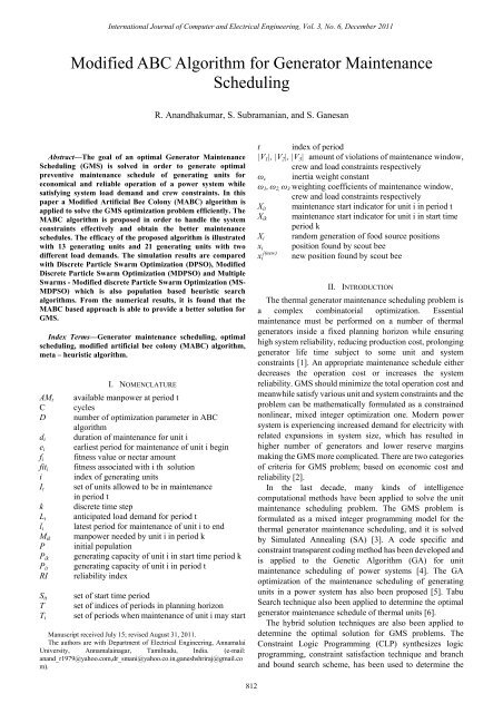
the weeks 28, 45, 46 and 52. From the comparison it is clear 

that the proposed MABC algorithm produce the better 

maintenance schedule in terms of attains maximum 

generation many times. The existing as well as the proposed 

algorithms is satisfying the load demand and crew 

requirements are exposed in Figs. 1 and 2. 

Available Generation (MW) 

DPSO MDPSO ABC 

Modified ABC Load Demand (5047 MW) Max. Generation (5688 MW) 

5800 

5600 

5400 

5200 

5000 

1 4 7 10 13 16 19 22 25 28 31 34 37 40 43 46 49 52 

Maintenace Period (Weeks) 

Fig. 1. Available generation of case 1 

DPSO MDPSO ABC Modified ABC Max. Crew (40) 

VII. SIMULATION RESULTS AND DISCUSSIONS 

This paper considers a test problem of scheduling 

maintenance of 21 generating units over a planning period of 

52 weeks and 13 generating units over a planning period of 

26 weeks. This test problem is loosely derived from the 

example presented in the literature [10], [11] and [12]. The 

performance of the proposed Modified ABC based generator 

maintenance scheduling algorithm is implemented using 

Matlab on a Intel (R) Core(TM) 2 Duo 2.10 GHz personal 

computer. The selected control parameters of ABC are 

N = 100, MCN =100 and Limit = 30. For Modified ABC, the 

control parameters are N=100, MCN=100 and Limit = 2501. 

A. Case 1: 21 Unit System [10] 

The proposed MABC algorithm is applied to GMS 

problem, with 21 generating units. The maintenance outages 

for the generating units are scheduled to minimize the sum of 

the squares of reserves and satisfying the following 

constraints. Maintenance window – each unit must be 

maintained exactly once every 52 weeks without interruption, 

the system peak load demand including 6.5% spinning 

reserve is 5047 MW, and there are 40 crew available each 

week for the maintenance work [8]. 

The maintenance schedule is obtained by DPSO, 

MDPSO, ABC and MABC is presented in Table 1. In the 

DPSO and MDPSO algorithm there is no low maintenance 

task for first 26 weeks i.e. entire 26 weeks the maintenance 

activities are carried out resulting in high available 

generation is not possible. Where as in ABC and MABC 

week 26 indicate period with low maintenance activity (no 

unit is scheduled for maintenance) resulting in comparatively 

high available generation on same week 26. In the last 26 

weeks, using the DPSO algorithm week 33 and using the 

MDPSO algorithm week 43 are indicate periods with low 

maintenance activity (no unit is scheduled for maintenance) 

resulting in comparatively high available generation on same 

weeks 33 and 43. Where as in ABC algorithm, weeks 28 and 

52 with low maintenance activity (no unit is scheduled for 

maintenance) resulting in comparatively high available 

generation on same weeks 28 and 52. The proposed MABC 

algorithm attains the maximum generation of 5688 MW in 

Crew 

45 

40 

35 

30 

25 

20 

15 

10 

5 

0 

1 11 21 31 41 51 

Maintenance Period (Weeks) 

Fig. 2. Crew requirements of case 1 

The convergence of the objective function (fitness) 

obtained over 5000 trials for ABC and MABC are presented 

in Fig. 3 and it is clear that the MABC converged quickly 

then ABC. 

Fitness 

9.00E+07 

8.00E+07 

7.00E+07 

6.00E+07 

5.00E+07 

4.00E+07 

3.00E+07 

2.00E+07 

1.00E+07 

0.00E+00 

1 1001 2001 3001 4001 5001 

Iterations 

ABC 

Fig. 3. Fitness versus iterations for case 1 

Modified ABC 

The Reliability Index (RI) given by Eq. (10) describes the 

degree of performance of the algorithms that results in 

optimal maintenance schedules. It is computed by taking the 

minimum of the ratio of available generation to load demand 

over 5000 trials and the entire operational period [8]. The 

functional aspect of the reliability indices is that they show 

the generation adequacy and the ability of the system to 

supply the aggregate electrical energy and meet demand 

requirements of the customers at all times during 

maintenance period. 

⎛ 

⎜ 

RI = Min( 

over5000trails) 

⎜Min( 

over52weeks) 

⎝ 

⎛ AvailGen . 

⎞⎞ 

⎜ if AvailGen . . ≤ Load⎟⎟ 

⎜ Load 

⎟⎟ 

⎝1 

otherwise ⎠⎠ 

(10) 

The RI s versus iterations for ABC and MABC are plotted 

in Fig. 4. 

815






0.95 

2.50E+07 

Reliability Index 

0.9 

0.85 

0.8 

0.75 

Fitness 

2.00E+07 

1.50E+07 

1.00E+07 

5.00E+06 

0.7 

1 1000 1999 2998 3997 4996 

Iterations 

0.00E+00 

1 1000 1999 2998 3997 4996 

Iterations 

Fig. 4. Reliability index versus iterations for case 1 

The MABC is seen to produce the most reliable schedule 

compared with ABC over 5000 trials. The result reveals that 

MABC produce better maintenance schedules then ABC. 

B. Case 2: 21 Unit System [11] 

In order to test the performance of the MABC algorithm, 

the same sample system is considered with the system peak 

load demand of 4739 MW, and 35 crew available each week 

for the maintenance work [11]. The complete maintenance 

schedule is obtained by MDPSO, MS-MDPSO, ABC and 

MABC is given in Table 2. 

In the MDPSO algorithm the weeks 23 & 35, the weeks 30 

& 36 in MS-MDPSO algorithm and the weeks 26, 33, 40 & 

52 in ABC and the weeks 25, 26, 32, 39, 40, 50, 51 & 52 in 

MABC represents the low maintenance activities that is no 

unit is scheduled for maintenance. From the comparison it is 

clear that the MABC algorithm produce the improved 

maintenance schedules then existing algorithms. The weekly 

available generation and crew requirements are depicted in 

Figs. 5 and 6 respectively. 


MDPSO MS-MDPSO ABC 

Modified ABC Load Demand (4739 MW) Max. Generation (5688 MW) 

5900 

5700 

5500 

5300 

5100 

4900 

4700 

1 11 21 31 41 51 



MDPSO MS-MDPSO ABC Modified ABC Max. Crew (35) 

Reliability Index 

0.95 

0.9 

0.85 

0.8 

0.75 

0.7 

0.65 

0.6 

Fig. 7. Fitness versus iterations for case 2 

1 1000 1999 2998 3997 4996 

Iterations 



Fig. 8. Reliability index versus iterations for case 2 

C. Case 3: 13 Unit System [12] 

The test system consists of 13 generating units with the 

system peak load with 6.5% spinning reserve is 2500 MW, 

available man power for maintenance per week is limited to 

40 and the maximum generation is 3150 MW [12]. The 

complete maintenance schedules obtained by DPSO, 

MDPSO and ABC are presented in Table 3. In DPSO and 

MDPSO algorithms entire 26 weeks the maintenance 

activities are carried out resulting in high available 

generation is not possible. The ABC algorithm reaches the 

high available generation of 3150 MW in week 13 since no 

units is scheduled for maintenance whereas the proposed 

MABC algorithm produce the better maintenance schedules 

in terms of attains the high available generation in the weeks 

14, 25 and 26. The weekly available generation and crew 

requirements are plotted in Fig. 9 & 10 respectively. From the 

comparison it is clear that the proposed ABC algorithm 

produce the better maintenance schedules than existing 

algorithms. 

DPSO MDPSO ABC MABC Max. Gen (3150 MW) Load (2500 MW) 

Crew 

40 

35 

30 

25 

20 

15 

10 

5 

0 

1 4 7 10 13 16 19 22 25 28 31 34 37 40 43 46 49 52 



3200 

2900 

2600 

2300 

1 6 11 16 21 26 




All the algorithms are satisfying the load requirements and 

crew requirements excepting MDPSO. The MDPSO 

algorithm does not satisfy the crew requirement on week 8 

due to heightened maintenance activities carried out 

simultaneously on units 3, 6 and 11. The convergence of the 

objective function and reliability index are presented in fig. 7 

& 8 respectively. The converged results clearly present 

minimization of the objective function and the optimization 

process demonstrates the capabilities of the MABC algorithm 

in minimizing large variations of system net reserve in case 

they occur 

Crew 

50 

40 

30 

20 

10 

0 

DPSO MDPSO ABC MABC Max. Crew (40) 

1 6 11 16 21 26 



816


TABLE I: GMS SCHEDULE FOR CASE 1 

WEEK NO 

GENERATING UNITS SCHEDULED FOR MAINTENANCE 


WEEK NO 

DPSO MDPSO ABC MABC DPSO MDPSO ABC MABC 

1 5 3,12 1 4 27 16 20 18 18,20 

2 5 2,12 1 4 28 16,18 16 ---- ---- 

3 5 2 1 4 29 16 16 14 16 

4 4 6 1 5 30 16 16 14 16 

5 4 6,9,13 1 5 31 16 16 14 16 

6 4 6,9,13 1 5 32 16 16 14 16 

7 3,6 6,13 1 1 33 --- 16 14 16 

8 6,10,13 6,7 5 1 34 20 19 16 16 

9 6,10,13 6,7,10 5 1,13 35 21 17,19 16 14 

10 6,10,13 6,7,10 5 1,13 36 21 17 16 14 

11 6,9,10 6,7,10 4 1,13 37 21 17 16 14 

12 6,9 6,7,11 4 1,11 38 21 14 16 14 

13 6 6,8,11 4 1,11 39 19 14 16 14 

14 6,7 5 6,13 6,10 40 19 14 19 19 

15 6,7 5 6,11,13 6,10 41 15 14 19,21 19,21 

16 6,7 5 6,11,13 6,10 42 15 14 21 17,21 

17 2,7 1 3,6 3,6,10 43 15 --- 21 17,21 

18 2,12 1 6,9,10 6,9 44 15 15 17,21 17,21 

19 8,12 1 6,9,10 6,9 45 15 15 17 --- 

20 1 1 6,8,10 6,8 46 17 15 17,20 --- 

21 1 1 6,10 6,7 47 17 15 15 15 

22 1 1 6,7 6,7 48 14,17 15 15 15 

23 1 1 6,7 6,7 49 14 21 15 15 

24 1 4 2,7,12 2,7,12 50 14 21 15 15 

25 1 4 2,7,12 2,12 51 14 21 15 15 

26 1 4 --- --- 52 14 18,21 ---- ---- 

WEEK 

NO 

TABLE II: GMS SCHEDULE FOR CASE 2 



WEEK 

MS - 

MS - 

MDPSO 

ABC MABC NO MDPSO 

ABC MABC 

MDPSO 

MDPSO 

1 1 12,13 8,10 1,10,13 27 19 17,20 17,21 15 

2 1 12,13 10 1,10,13 28 19,20 17,19 17,21 15 

3 1 4,13 1,10 1,10,13 29 16 17,19 17,21 15 

4 1 4 1,10 1,10 30 16 --- 21 15 

5 1 4 1 1,11 31 16 14 19 15 

6 1 2,6 1 1,11 32 16 14 19 --- 

7 1,6 2,6 1 1 33 16 14 --- 16,18 

8 3,6,11 6 1 --- 34 16 14 14 16 

9 2,6,11 6 1 4 35 --- 14 14 16 

10 2,6 6,7,8 2 2,4 36 17 --- 14 16 

11 6 6,7 2,4 2,4 37 17 21 14 16 

12 6 6,7 4 5,9 38 17 21 14 16 

13 6,13 6,7 4,9 5,9 39 14 21 20 --- 

14 6,10,13 6,7,11 5,9 5 40 14 21 --- --- 

15 6,10,13 6,11 3,5 3,6 41 14 18 16 14,19 

16 6,7,10 6 5,6 6 42 14 16 16 14,19 

17 7,10 6 6 6 43 14 16 16 14 

18 7,9,12 5,9 6 6 44 21 16 16,18 14 

19 7,9,12 5,9 6,12,13 6,12 45 18,21 16 16 14 

20 4 1 6,12,13 6,12 46 21 16 16 20,21 

21 4 1 6,11,13 6,7 47 21 16 15 17,21 

22 4 1,10 6,7,11 6,7 48 15 15 15 17,21 

23 --- 1,10 6,7 6,7 49 15 15 15 17,21 

24 5 1,10 6,7 6,7,8 50 15 15 15 --- 

25 5 1,10 6,7 ---- 51 15 15 15 --- 

26 5,8 1 --- ---- 52 15 15 --- --- 

817


WEEK 

NO 

TABLE III: GMS SCHEDULE FOR CASE 3 


DPSO MDPSO ABC MABC 

1 4 4 2,6 1,10 

2 4 4 2,6 1,10 

3 4 4 6,3 1,10 

4 6 6 6,7 1,10 

5 6,7 2,6,13 6,7 1,11,13 

6 6,7 2,6,13 6,7 1,11,13 

7 2,6,7 6,13 6,7 1,13 

8 2,6,7 3,6 6,13 4 

9 3,6,13 6,12 6,13 4 

10 6,13 6,11,12 6,13 4 

11 6,10 6,10,11 11,12 5 

12 6,10 6,10 11,12 5 

13 6,10,11 6,7,10 ---- 5 

14 10,11 7,10 4 ---- 

15 12 7 4 2,6,7 

16 12 7,8 4 2,6,7 

17 5 5 5 6,7 

18 5 5 5 6,7 

19 5 5 5 6,8 

20 1 1 1,8 6,9 

21 1 1 1,9 6,9 

22 1 1 1,9 6,12 

23 1 1 1,10 6,12 

24 1,8 1 1,10 6,3 

25 1,9 1,9 1,10 --- 

26 1,9 1,9 1,10 --- 

VIII. CONCLUSION 

The problem of generating optimal maintenance schedules 

of generating units for the purpose of maximizing economic 

benefits and improving reliable operation of a power system, 

subject to satisfying system constraints. In this paper, a 

Modified Artificial Bee Colony (MABC) algorithm is 

proposed to solve a challenging power system optimization 

problem of generating unit maintenance schedule. The 

MABC is a novel bio inspired algorithm suitable for 

engineering optimization problems, which is simple, robust 

and efficient in handling the constraints and produce better 

maintenance schedules. The modifications are made in the 

initialization stage and control parameter (limit) of the ABC 

algorithm, however these do not alter but improve the 

inherent search process of the algorithm. The performance of 

the proposed algorithm for solving GMS is tested with the 13 

and 21 unit test system and the results are compared with 

earlier reported methods. It is evident from the comparison 

the Modified ABC provides a competitive performance in 

terms of optimal solution. It is also found that this method is 

to be a promising alternative approach for solving GMS 

problems in practical power system. 

ACKNOWLEDGMENT 

The authors gratefully acknowledge the management the 

support and facilities provided by the authorities of 

Annamalai University, Annamalainagar, India to carry out 

this research work. 

REFERENCES 

[1] A. J. Wood and B. F. Wollenberg, Power generation operation and 

control, New York: John Wiley and Sons, 1996. 

[2] R. Mukerji, H. M. Merrill, B. W. Erickson, and J. H. Parker, “Power 

plant maintenance scheduling: Optimizing economics and reliability,” 

IEEE Trans. Power Systems, Vol. 6, pp. 476-483, May 1991. 

[3] T. Satoh and K. Nara, “Maintenance scheduling by using simulated 

annealing method,” IEEE Trans. Power Systems, Vol. 6, pp. 850-857, 

May 1991. 

[4] Y. Wang and E. Handschin, “A new genetic algorithm for preventive 

unit maintenance scheduling of power systems,” Elect. Power Ener. 

Syst, Vol. 22, pp. 343-348, 2000. 

[5] A. Volkanovski, B. Mavko, T. Boševski, A. Čauševski, and M. Čepin, 

“Genetic algorithm optimization of the maintenance scheduling of 

generating units in a power system,” Reliab. Eng. Syst. Safety, Vol. 93, 

pp. 757-767, 2008. 

[6] I. El-Amin, S. Duffuaa, and M. Abbas, “A Tabu search algorithm for 

maintenance scheduling of generating units,” Elect. Power Syst. Res., 

Vol. 54, pp. 91- 99, 2000. 

[7] K. Y. Huang and H. T. Yang, “Effective algorithm for handling 

constraints in generator maintenance scheduling,” IEE Proc. 

Generation, Transmission and Distribution, Vol. 149, pp. 274-282, 

May 2002. 

[8] K. P. Dahal and N. Chakpitak, “Generator maintenance scheduling in 

power systems using metaheuristic-based hybrid approaches,” Elect. 

Power Syst. Res, Vol. 77, pp. 771-779, 2007. 

[9] S. P. Canto, “Application of Benders’ decomposition to power plant 

preventive maintenance scheduling,” Europ. J. Oper. Res. Vol. 184, pp. 

759-777, 2008. 

[10] Y. Yare, G. K. Venayagamoorthy, and U. O. Aliyu, “Optimal generator 

maintenance scheduling using a modified discrete PSO,” IET Gener. 

Transm. Distrib. Vol. 2, pp. 834-846, May 2008. 

[11] Y. Yare and G. K. Venayagamoorthy, “Optimal-maintenance 

scheduling of generators using multiple swarms-MDPSO framework,” 

Engg. App. Artifi. Intelli, Vol. 23, pp. 895-910, 2010. 

[12] Yusuf Yare and Ganesh K. Venayagamoorthy, “Optimal scheduling of 

generator maintenance using modified discrete particle swarm 

optimization,” Proceedings of IEEE on iREP Symposium, August 

19-24, Charleston, SC, USA, 2007. 

[13] D. Karaboga and B. Basturk, “On the performance of Artificial Bee 

Colony (ABC) Algorithm,” App. Soft Comput, Vol. 8, pp. 687-697, 

2008. 

[14] Z. Changsheng, O. Dantong, and N. Jiaxu, “An artificial bee colony 

approach for clustering,” Expert Syst. with App, Vol. 37, pp. 4761-4767, 

2010. 

[15] A. Bilal, “Chaotic bee colony algorithms for global numerical 

optimization,” Expert Syst. with App, Vol. 37, pp. 5682-5687, 2010. 

[16] S. L. Sabat, S. K. Udgata, and A. Abraham, “Artificial bee colony 

algorithm for small signal model parameter extraction of MESFET,” 

Engg. App. of Artifi. Intelli, Vol. 23, pp. 689-694, 2010. 

818


R.Anandhakumar received the B.E degree in 

Electrical and Electronics Engineering and the 

M.E degree in Power Systems with distinction 

from Annamalai University, Annamalainagar, 

India in the year 2000 and 2008 respectively. He 

is currently with the Department of Electrical 

Engineering as a Assistant Professor. His research 

interests include power system operation and 

control and computational intelligence applications. 

He published 130 research articles in various referred international 

journals, national journals, international conferences and national 

conferences. He is a review committee member for various international and 

national journals. His area of interest includes power system operation and 

control, design analysis of electrical machines, power system state estimation 

and power system voltage stability studies. His biography has been included 

in MARQUIS who is who in the world, MARQUIS who is who in 

Engineering and International Biographical Centre (IBC), UK. He received 

the best teacher award in recognition of his research contributions in 

Annamalai University. 

S. Subramanian is a Professor with the 

Department of Electrical Engineering, Annamalai 

University, Annamalainagar, India. He is a Senior 

member in IEEE, Fellow of Institution of 

Engineers (India) and a member of various 

professional bodies such as System Society of 

India, India Society for Technical Education and 

Indian Science Congress Association. He received 

the B.E degree in Electrical and Electronics 

Engineering and the M.E degree in Power Systems with distinction from 

Madurai Kamaraj University, Madurai, India in the year 1989 and 1990 

respectively. He received the Ph.D degree in the year 2001 from Annamalai 

University, Annamalainagar, India. 

S. Ganesan is working as an Assistant Professor 

in the Department of Electrical Engineering, 

Annamalai University. He received the B.E degree 

in Electrical and Electronics Engineering from 

Government College of Engineering, Salem, India 

in 2002 and M.E degree in Power Systems with 

distinction in the year 2008 from Annamalai 

University, Annamalainagar, India. He is currently 

pursuing Ph.D degree (Part-time) in the 

Department of Electrical Engineering, Annamalai University, 

Annamalainagar, India. His research topics include power systems operation 

and control. 

819

Modified ABC Algorithm for Generator Maintenance Scheduling - ijcee

You also want an ePaper? Increase the reach of your titles

Delete template?

Save as template?