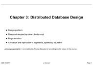
Chapter 6: Query Decomposition and Data Localization

Chapter 6: Query Decomposition and Data 

Localization 

• Query Decomposition 

• Data Localization 

Acknowledgements: I am indebted to Arturas Mazeika for providing me his slides of this course. 

DDB 2008/09 J. Gamper Page 1

Query Decomposition 

• Query decomposition: Mapping of calculus 

query (SQL) to algebra operations (select, 

project, join, rename) 

• Both input and output queries refer to global relations, 

without knowledge of the distribution of 

data. 

• The output query is semantically correct and 

good in the sense that redundant work is 

avoided. 

• Query decomposistion consists of 4 steps: 

1. Normalization: Transform query to a normalized form 

2. Analysis: Detect and reject ”incorrect” queries; possible only for a subset of relational 

calculus 

3. Elimination of redundancy: Eliminate redundant predicates 

4. Rewriting: Transform query to RA and optimize query 


Query Decomposition – Normalization 

• Normalization: Transform the query to a normalized form to facilitate further processing. 

Consists mainly of two steps. 

1. Lexical and syntactic analysis 

– Check validity (similar to compilers) 

– Check for attributes and relations 

– Type checking on the qualification 

2. Put into normal form 

– With SQL, the query qualification (WHERE clause) is the most difficult part as it 

might be an arbitrary complex predicate preceeded by quantifiers (∃, ∀) 

– Conjunctive normal form 

(p 11 ∨ p 12 ∨ · · · ∨ p 1n ) ∧ · · · ∧ (p m1 ∨ p m2 ∨ · · · ∨ p mn ) 

– Disjunctive normal form 

(p 11 ∧ p 12 ∧ · · · ∧ p 1n ) ∨ · · · ∨ (p m1 ∧ p m2 ∧ · · · ∧ p mn ) 

– In the disjunctive normal form, the query can be processed as independent 

conjunctive subqueries linked by unions (corresponding to the disjunction) 


Query Decomposition – Normalization . . . 

• Example: Consider the following query: Find the names of employees who have been 

working on project P1 for 12 or 24 months? 

• The query in SQL: 

SELECT ENAME 

FROM EMP, ASG 

WHERE EMP.ENO = ASG.ENO AND 

ASG.PNO = ‘‘P1’’ AND 

DUR = 12 OR DUR = 24 

• The qualification in conjunctive normal form: 

EMP.ENO = ASG.ENO ∧ ASG.PNO = ”P1” ∧ (DUR = 12 ∨ DUR = 24) 

• The qualification in disjunctive normal form: 

(EMP.ENO = ASG.ENO ∧ ASG.PNO = ”P1” ∧ DUR = 12) ∨ 

(EMP.ENO = ASG.ENO ∧ ASG.PNO = ”P1” ∧ DUR = 24) 


Query Decomposition – Analysis 

• Analysis: Identify and reject type incorrect or semantically incorrect queries 

• Type incorrect 

– Checks whether the attributes and relation names of a query are defined in the global 

schema 

– Checks whether the operations on attributes do not conflict with the types of the 

attributes, e.g., a comparison > operation with an attribute of type string 

• Semantically incorrect 

– Checks whether the components contribute in any way to the generation of the result 

– Only a subset of relational calculus queries can be tested for correctness, i.e., those 

that do not contain disjunction and negation 

– Typical data structures used to detect the semantically incorrect queries are: 

∗ Connection graph (query graph) 

∗ Join graph 


Query Decomposition – Analysis . . . 

• Example: Consider a query: 

SELECT ENAME,RESP 

FROM EMP, ASG, PROJ 

WHERE EMP.ENO = ASG.ENO 

AND ASG.PNO = PROJ.PNO 

AND PNAME = "CAD/CAM" 

AND DUR ≥ 36 

AND TITLE = "Programmer" 

• Query/connection graph 

– Nodes represent operand or result relation 

– Edge represents a join if both connected 

nodes represent an operand relation, otherwise 

it is a projection 

• Join graph 

– a subgraph of the query graph that considers 

only the joins 

• Since the query graph is connected, the query is semantically correct 


Query Decomposition – Analysis . . . 

• Example: Consider the following query and its query graph: 

SELECT ENAME,RESP 

FROM EMP, ASG, PROJ 

WHERE EMP.ENO = ASG.ENO 

AND PNAME = "CAD/CAM" 

AND DUR ≥ 36 

AND TITLE = "Programmer" 

• Since the graph is not connected, the query is semantically incorrect. 

• 3 possible solutions: 

– Reject the query 

– Assume an implicit Cartesian Product between ASG and PROJ 

– Infer from the schema the missing join predicate ASG.PNO = PROJ.PNO 


Query Decomposition – Elimination of Redundancy 

• Elimination of redundancy: Simplify the query by eliminate redundancies, e.g., 

redundant predicates 

– Redundancies are often due to semantic integrity constraints expressed in the query 

language 

– e.g., queries on views are expanded into queries on relations that satiesfy certain 

integrity and security constraints 

• Transformation rules are used, e.g., 

– p ∧ p ⇐⇒ p 

– p ∨ p ⇐⇒ p 

– p ∧ true ⇐⇒ p 

– p ∨ false ⇐⇒ p 

– p ∧ false ⇐⇒ false 

– p ∨ true ⇐⇒ true 

– p ∧ ¬p ⇐⇒ false 

– p ∨ ¬p ⇐⇒ true 

– p 1 ∧ (p 1 ∨ p 2 ) ⇐⇒ p 1 

– p 1 ∨ (p 1 ∧ p 2 ) ⇐⇒ p 1 


Query Decomposition – Elimination of Redundancy . . . 

• Example: Consider the following query: 

SELECT TITLE 

FROM EMP 

WHERE EMP.ENAME = "J. Doe" 

OR (NOT(EMP.TITLE = "Programmer") 

AND ( EMP.TITLE = "Elect. Eng." 

OR EMP.TITLE = "Programmer" ) 

AND NOT(EMP.TITLE = "Elect. Eng.")) 

• Let p 1 be ENAME = ”J. Doe”, p 2 be TITLE = ”Programmer” and p 3 be TITLE = ”Elect. 

Eng.” 

• Then the qualification can be written as p 1 ∨ (¬p 2 ∧ (p 2 ∨ p 3 ) ∧ ¬p 3 ) 

and then be transformed into p 1 

• Simplified query: 

SELECT TITLE 

FROM EMP 

WHERE 

EMP.ENAME = "J. Doe" 


Query Decomposition – Rewriting 

• Rewriting: Convert relational calculus query to relational algebra query and find an 

efficient expression. 

• Example: Find the names of employees other 

than J. Doe who worked on the CAD/CAM 

project for either 1 or 2 years. 

• SELECT 

FROM 

WHERE 

AND 

AND 

AND 

ENAME 

EMP, ASG, PROJ 

EMP.ENO = ASG.ENO 

ASG.PNO = PROJ.PNO 

ENAME ≠ "J. Doe" 

PNAME = "CAD/CAM" 

AND (DUR = 12 OR DUR = 24) 

• A query tree represents the RA-expression 

– Relations are leaves (FROM clause) 

– Result attributes are root (SELECT clause) 

– Intermediate leaves should give a result 

from the leaves to the root 


Query Decomposition – Rewriting . . . 

• By applying transformation rules, many different trees/expressions may be found that 

are equivalent to the original tree/expression, but might be more efficient. 

• In the following we assume relations R(A 1 , . . . , A n ), S(B 1 , . . . , B n ), and T which is 

union-compatible to R. 

• Commutativity of binary operations 

– R × S = S × R 

– R ⋊⋉ S = S ⋊⋉ R 

– R ∪ S = S ∪ R 

• Associativity of binary operations 

– (R × S) × T = R × (S × T) 

– (R ⋊⋉ S) ⋊⋉ T = R ⋊⋉ (S ⋊⋉ T) 

• Idempotence of unary operations 

– Π A (Π A (R)) = Π A (R) 

– σ p1(A1) (σ p2(A2) (R)) = σ p1(A1)∧p2(A2) (R) 



• Commuting selection with binary operations 

– σ p(A) (R × S) ⇐⇒ σ p(A) (R) × S 

– σ p(A1 )(R ⋊⋉ p(A2 ,B 2 ) S) ⇐⇒ σ p(A1 )(R) ⋊⋉ p(A2 ,B 2 ) S 

– σ p(A) (R ∪ T) ⇐⇒ σ p(A) (R) ∪ σ p(A) (T) 

∗ (A belongs to R and T ) 

• Commuting projection with binary operations (assume C = A ′ ∪ B ′ , 

A ′ ⊆ A, B ′ ⊆ B) 

– Π C (R × S) ⇐⇒ Π A ′(R) × Π B ′(S) 

– Π C (R ⋊⋉ p(A ′ ,B ′ ) S) ⇐⇒ Π A ′(R) ⋊⋉ p(A ′ ,B ′ ) Π B ′(S) 

– Π C (R ∪ S) ⇐⇒ Π C (R) ∪ Π C (S) 



• Example: Two equivalent query trees for the previous example 

– Recall the schemas: EMP(ENO, ENAME, TITLE) 

PROJ(PNO, PNAME, BUDGET) 

ASG(ENO, PNO, RESP, DUR) 



• Example (contd.): Another equivalent query tree, which allows a more efficient query 

evaluation, since the most selective operations are applied first. 


Data Localization 

• Data localization 

– Input: Algebraic query on global conceptual 

schema 

– Purpose: 

∗ Apply data distribution information to the 

algebra operations and determine which 

fragments are involved 

∗ Substitute global query with queries on 

fragments 

∗ Optimize the global query 


Data Localization . . . 

• Example: 

– Assume EMP is horizontally fragmented 

into EMP1, EMP2, EMP3 as follows: 

∗ EMP1 = σ ENO≤”E3” (EMP) 

∗ EMP2 = σ ”E3””E6” (EMP) 

– ASG fragmented into ASG1 and ASG2 as 

follows: 

∗ ASG1 = σ ENO≤”E3” (ASG) 

∗ ASG2 = σ ENO>”E3” (ASG) 

• Simple approach: Replace in all queries 

– EMP by (EMP1∪EMP2∪ EMP3) 

– ASG by (ASG1∪ASG2) 

– Result is also called generic query 

• In general, the generic query is inefficient since important restructurings and 

simplifications can be done. 



• Example (contd.): Parallelsim in the evaluation is often possible 

– Depending on the horizontal fragmentation, the fragments can be joined in parallel 

followed by the union of the intermediate results. 



• Example (contd.): Unnecessary work can be eliminated 

– e.g., EMP 3 ⋊⋉ ASG 1 gives an empty result 

∗ EMP3 = σ ENO>”E6” (EMP) 



Data Localizations Issues 

• Various more advanced reduction techniques are possible to generate simpler and 

optimized queries. 

• Reduction of horizontal fragmentation (HF) 

– Reduction with selection 

– Reduction with join 

• Reduction of vertical fragmentation (VF) 

– Find empty relations 


Data Localizations Issues – Reduction of HF 

• Reduction with selection for HF 

– Consider relation R with horizontal fragmentation F = {R 1 , R 2 , . . . , R k }, where 

R i = σ pi (R) 

– Rule1: Selections on fragments, σ pj (R i ), that have a qualification contradicting the 

qualification of the fragmentation generate empty relations, i.e., 

σ pj (R i ) = ∅ ⇐⇒ ∀x ∈ R(p i (x) ∧ p j (x) = false) 

– Can be applied if fragmentation predicate is inconsistent with the query selection 

predicate. 

• Example: Consider the query: SELECT * FROM EMP WHERE ENO=”E5” 

After commuting the selection 

with the union operation, 

it is easy to detect that the 

selection predicate contradicts 

the predicates of EMP 1 

and EMP 3 . 


Data Localizations Issues – Reduction for HF . . . 

• Reduction with join for HF 

– Joins on horizontally fragmented relations can be simplified when the joined relations 

are fragmented according to the join attributes. 

– Distribute join over union 

(R 1 ∪ R 2 ) ⋊⋉ S ⇐⇒ (R 1 ⋊⋉ S) ∪ (R 2 ⋊⋉ S) 

– Rule 2: Useless joins of fragments, R i = σ pi (R) and R j = σ pj (R), can be 

determined when the qualifications of the joined fragments are contradicting, i.e., 

R i ⋊⋉ R j = ∅ ⇐⇒ ∀x ∈ R i , ∀y ∈ R j (p i (x) ∧ p j (y) = false) 

∪ 

⋊⋉ 

R i 

R 1 R 2 R 3 

⋊⋉ pi ,p 1 

∪ 

⋊⋉ pi ,p 2 

⋊⋉ pi ,p 3 

R i R 1 R i R 2 R i R 3 



• Example: Consider the following query and fragmentation: 

– Query: SELECT * FROM EMP, ASG WHERE EMP.ENO=ASG.ENO 

– Horizontal fragmentation: 

∗ EMP1 = σ ENO≤”E3” (EMP) 

∗ EMP2 = σ ”E3””E6” (EMP) 


∗ ASG2 = σ ENO>”E3” (ASG) 

– Generic query 

– The query reduced by distributing 

joins over unions and applying 

rule 2 can be implemented 

as a union of three partial joins 

that can be done in parallel. 



• Reduction with join for derived HF 

– The horizontal fragmentation of one relation is derived from the horizontal 

fragmentation of another relation by using semijoins. 

• If the fragmentation is not on the same predicate as the join (as in the previous 

example), derived horizontal fragmentation can be applied in order to make efficient join 

processing possible. 

• Example: Assume the following query and fragmentation of the EMP relation: 

– Query: SELECT * FROM EMP, ASG WHERE EMP.ENO=ASG.ENO 

– Fragmentation (not on the join attribute): 

∗ EMP1 = σ TITLE=“Prgrammer” (EMP) 

∗ EMP2 = σ TITLE≠“Prgrammer” (EMP) 

– To achieve efficient joins ASG can be fragmented as follows: 

∗ ASG1= ASG⊲< ENO EMP1 

∗ ASG2= ASG⊲< ENO EMP2 

– The fragmentation of ASG is derived from the fragmentation of EMP 

– Queries on derived fragments can be reduced, e.g., ASG 1 ⋊⋉ EMP 2 = ∅ 


Data Localizations Issues – Reduction for VF 

• Reduction for Vertical Fragmentation 

– Recall, VF distributes a relation based on projection, and the reconstruction operator 

is the join. 

– Similar to HF, it is possible to identify useless intermediate relations, i.e., fragments 

that do not contribute to the result. 

– Assume a relation R(A) with A = {A 1 , . . . , A n }, which is vertically fragmented as 

R i = π A 

′ 

i 

(R), where A ′ i ⊆ A. 

– Rule 3: π D,K (R i ) is useless if the set of projection attributes D is not in A ′ i and K 

is the key attribute. 

– Note that the result is not empty, but it is useless, as it contains only the key attribute. 


Data Localizations Issues – Reduction for VF . . . 

• Example: Consider the following query and vertical fragmentation: 

– Query: SELECT ENAME FROM EMP 

– Fragmentation: 

∗ EMP1 = Π ENO,ENAME (EMP) 

∗ EMP2 = Π ENO,TITLE (EMP) 

• Generic query 

• Reduced query 

– By commuting the projection with the join (i.e., projecting 

on ENO, ENAME), we can see that the projection 

on EMP 2 is useless because ENAME is not 

in EMP 2 . 


Conclusion 

• Query decomposition and data localization maps calculus query into algebra operations 

and applies data distribution information to the algebra operations. 

• Query decomposition consists of normalization, analysis, elimination of redundancy, and 

rewriting. 

• Data localization reduces horizontal fragmentation with join and selection, and vertical 

fragmentation with joins, and aims to find empty relations.

Chapter 6: Query Decomposition and Data Localization

You also want an ePaper? Increase the reach of your titles

Delete template?

Save as template?