Tutorial slides

EDBT Summer School 

Database Performance 

Pat & Betty (Elizabeth) O’Neil 

Sept. 6, 2007

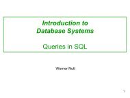
Database Performance: Outline 

 

 

 

 

 

 

Here is an outline of our two-lecture course 

First, we explain why OLTP performance is no longer thought to 

be an important problem by most researchers and developers 

But we’ll introduce a new popular Transactional product called 

Snapshot Isolation that supports updates & concurrent queries 

Then we look at queries, especially Data Warehouse queries, 

which get the most performance attention currently 

We explain early query performance concepts, e.g. index Filter 

Factor, then look at cubical clustering, the new crucial factor 

Data Warehousing is where most new purchases are made at 

present, and we examine the area in detail 

2

DB Performance: OLTP 

Jim Gray said years ago: OLTP is a solved problem 

Older established companies that do OLTP Order Entry have 

solutions in place, efficient enough not to need change 

One reason is that change is very difficult: rewriting a company’s 

OLTP programs is called the “Dusty Decks” problem 

Nobody remembers how all the code works! 

Also, the cost of hardware to support update transactions 

compared to programming costs, or even terminal costs, is low 

We explain this in the slides immediately following 

But some new installations use new transactional approaches 

that better support queries, such as Snapshot Isolation 

We explain Snapshot Isolation a bit later (starting on Slide 7) 

3

OLTP DebitCredit Benchmark 

Anon [Jim Gray] et al. paper (in Datamation, 1985) 

introduced the DebitCredit benchmark. 

Bank Transaction tables: Acct, Teller, Brnch, History, with 100 byte rows 

Read 100 bytes from terminal: aid, tid, bid, delta 

Begin Transaction; 

Update Accnt set Accnt_bal = Accnt_bal +:delta where Accnt_ID = :aid; 

Insert to History values (:aid,:tid, :bid, :delta, Time_stamp); 

Update Teller set Teller_bal = Teller_bal + :delta where Teller_ID = :tid; 

Update Brnch set Brnch_bal = Brnch_bal+:delta where Brnch_ID = :bid; 

Commit; 

Write 200 bytes to terminal including: aid, tid, bid, delta, Accnt_bal 

Transactions per second (tps) scaled with size of tables: each tps had 

100,000 Accnts, 10 Brnches, 100 Tellers; History held 90 days of inserts 

1 History of DebitCredit/TPC-A in Jim Gray’s “The Benchmark Handbook”, Chapter 2. 

4

OLTP DebitCredit Benchmark 

 

 

 

 

 

 

 

DebitCredit restrictions; performance features tested 

Terminal request response time required 95% under 1 second; 

throughput driver had to be titrated to give needed response 

Think time was 100 secs (after response): meant much context 

had to be held in memory for terminals (10,000 for 100 tps) 

Terminal simulators were used; Variant TP1 benchmark drove 

transactions by software loop generation with trivial think time 

Mirrored Tx logs required to provide guaranteed recovery 

History Inserts (50 byte rows) costly if pages locked 

System had to be priced, measured in $/tps 

5

OLTP DebitCredit/TPC-A Benchmark 

 

 

 

 

Vendors cheated when running DebitCredit 

Jim Gray welcomed new Transaction Processing Performance 

Council (TPC), consortium of vendors, created TPC-A 1 in 1989 

Change from DebitCredit: measurement rules were carefully 

specified and auditors were required for results to be published 

Detail changes: 

For each 1 tps, only one Branch instead of 10: meant concurrency 

would be tougher: important to update Branch LAST 

Instead of 100 sec Think Time, used 10 sec. Unrealistic, but reason 

was that TERMINAL PRICES WERE TOO HIGH WITH 100 SEC! 

Terminal prices were more than all other costs for benchmark 

Even in 1989, transactions were cheap to run! 

1 History of DebitCredit/TPC-A in Jim Gray’s “The Benchmark Handbook”, Chapter 2. In ACM 

SIGMOD Anthology, http://www.sigmod.org/dblp/db/books/collections/gray93.html 

6

DB Performance: OLTP & Queries 

 

 

 

 

 

 

Amazon doesn’t use OLTP of any DBMS to enter purchases in 

a customer’s shopping cart (does for dollar transactions though) 

Each purchase is saved using a PC file system, with mirroring & 

replication for failover in case of node drop-out: log not needed 

Classical OLTP not needed because only one purchase saved 

at a time on a single-user shopping cart 

There is one new approach to transactional isolation adopted for 

some new applications, mainly used to support faster queries 

It is called “Snapshot Isolation” 1 (SI), and it has been adopted in 

both the Oracle and Microsoft SQL Server database products 

SI is not fully Serializable, so it is officially an Isolation Level, but 

anomalies are rare and Queries aren’t blocked by Update Tx’s 

1 First published in SIGMOD 2005. A Critique of ANSI Isolation Levels. by Hal Berenson, Phil 

Bernstein, Jim Gray, Jim Melton, Pat O’Neil and Elizabeth O’Neil 

7

DB Performance: Snapshot Isolation (SI) 

 

 

 

 

 

 

A transaction T i executing under Snapshot Isolation (SI) reads 

only committed data as of the time Start(T i ) 

This doesn’t work by taking a “snapshot” of all data when new 

Tx starts, but by taking a timestamp and keeping old versions of 

data when new versions are written: Histories in SI read & write 

“versions” of data items 

Data read, including both row values and indexes, time travels 

to Start(T i ), so predicates read by T i also time travel to Start(T i ) 

A transaction T i in SI also maintains data it has written in a local 

cache, so if it rereads this data, it will read what it wrote 

No T k concurrent with T i (overlapping lifetimes) can read what T i 

has written (can only read data committed as of Start(T k )) 

If concurrent transactions both update same data item A, then 

second one trying to commit will abort (First committer wins rule) 

8

DB Performance: Snapshot Isolation (SI) 

 

 

 

 

 

 

SI Histories read and write Versions of data items: (X0, X1, X2); 

X0 is value before updates, X2 would be written by T 2 , X7 by T 7 

Standard Tx’l anomalies of non-SR behavior don’t occur in SI 

Lost Update anomaly in Isolation Level READ COMMITTED 

(READ COMMITTED is Default Isolation Level on all DB products) : 

(I’m underlining T 2 ’s operations just to group them visually) 

H1: R 1 (X,50) R 2 (X,50) W 2 (X,70) C 2 W 1 (X,60) C 1 (X should be 80) 

In SI, First Committer Wins property prevents this anomaly: 

H1 SI : R 1 (X0,50) R 2 (X0,50) W 2 (X2,70) C 2 W 1 (X1,60) A 1 

Inconsistent View anomaly possible in READ COMMITTED: 

H2: R 1 (X,50) R 2 (X,50) W 2 (X,70) R 2 (Y,50) W 2 (Y,30) C 2 R 1 (Y,30) C 1 

Here T1 sees X+Y = 80; In SI, Snapshot Read avoids this anomaly 

H2 SI : R 1 (X0,50) R 2 (X0,50) W 2 (X2,70) R 2 (Y0,50) W 2 (Y2,30) C 2 

R 1 (Y0,50) C 1 (T 1 reads sum of X+Y = 100, valid at Start(T 1 ) 

9

DB Performance: Snapshot Isolation 

In SI, READ-ONLY T 1 never has to wait for Update T 2 

since T 1 reads consistent committed data at Start(T 1 ) 

Customers LIKE this property! 

SI was adopted by Oracle to avoid implementing DB2 

Key Value Locking that prevents predicate anomalies 

In SI, new row insert by T 2 into predicate read by T 1 

won’t be accessed by T 1 (since index entries have 

versions as well) 

Customers using Oracle asked Microsoft to adopt SI 

as well, so Readers wouldn’t have to WAIT 

10


 

 

 

 

 

Oracle calls the SI Isolation Level “SERIALIZABLE” 

SI is not truly SERIALIZABLE (SR); anomalies exist 

Assume husband and wife have bank account balances A and B 

with starting values 100; Bank allows withdrawals from these 

accounts to bring balances A or B negative as long as A+B > 0 

This is a weird constraint; banks probably wouldn’t impose it 

In SI can see following history: 

H3: R 1 (A0,100) R 1 (B0,100) R 2 (A0,100) R 2 (B0,100) W 2 (A2,-30) C 2 

W 1 (B1,-30) C 1 

Both T 1 and T 2 expect total balance will end positive, but it goes 

negative because each Tx has value it read changed by other Tx 

This is called a “Skew Writes” anomaly: weird constraint fails 

11

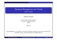
Snapshot Isolation Skew-Write Anomaly 

R 1 (A0,100) R 1 (B0,100) R 2 (A0,100) R 2 (B0,100) W 2 (A2,-30) C 2 W 1 (B1,-30) C 1 

R 1 (A0,100) R 1 (B0,100) 

T1 

W 1 (B1,-30) C 1 

T2 

Conflict cycle 

allowed by SI 

R 2 (A0,100) R 2 (B0,100) W 2 (A2,-30) C 2 

Time-->


 

 

Here is a Skew Write anomaly with no pre-existing constraint 

Assume T 1 copies data item X to Y and T 2 copies Y to X 

R 1 (X0,10) R 2 (Y0,20) W 1 (Y1,10) C 1 W 2 (X2,20) C 2 

Concurrent T 1 & T 2 only exchange values of X and Y 

 

 

But any serial execution of T 1 & T 2 would end with X and Y 

identical, so this history is not SR 

Once again we see an example of skew writes: each concurrent 

Tx depends on value that gets changed 

The rule (constraint?) broken is quite odd, and unavoidable: it is 

one that comes into existence only as a post-condition! 

13


 

 

 

 

 

SI anomalies rarely occur in commercial applications 

Oracle called SI “SERIALIZABLE” when they learned it had no 

anomalies in the (Tx’l) TPC-C benchmark 

It is also usually possible to prevent SI anomalies with proper 

forethought 1 : here is Skew Write anomaly 

R 1 (X0,10) R 2 (Y0,20) W 1 (Y1,10) C 1 W 2 (X2,20) C 2 

Can “Select For Update” Oracle, like Writing same value so 

Crucial read is stable (symbolize below with RU) 

RU 1 (X0,10) RU 2 (Y0,20) W 1 (Y1,10) C 1 W 2 (X2,20) A 2 

SI shows there is transactional research possible, but ANTS 

product writeup 1 seems to push OLTP performance to its limit! 

1 For details see: A. Fekete, D. Liarokapis, E. O’Neil, P. O’Neil and D. Shasha. 

Making Snapshot Isolation Serializable. ACM TODS, Vol 30, No. 2, June 2005 

2 Download from http://www.cs.umb.edu/~poneil/ANTS.pdf 

14

DB Performance: Queries 

Companies are spending the most money now on 

developing query systems, with few, if any, updates 

I’ll start with some historical development 

E. F. Codd’s Relational Paper was published in 1970; 

Codd worked at IBM; DB2 was first released in 1982 

SEQUEL, early SQL, was published 1 in 1974 for 

use in IBM’s System R, a DB2 precursor 

ORACLE (then Relational Software, Inc.) put out a 

commercial version of SQL in 1979 

1 

Donald Chamberlin and Raymond Boyce, 1974. SEQUEL: A Structured English Query 

Language. SIGFIDET (later SIGMOD), pp. 249-264. 

15

DB Performance: Early DB2 & M204 

DB2 Query Indexes were explained in 1979 paper 1 

 

 

 

 

Rather primitive: Choose single column restriction that gives 

smallest “selectivity factor” F 

Selectivity factor was later “Filter Factor” in documentation 

The ability to AND Filter Factors waited until DB2 V2, 1988 

After DB2 was introduced, Pat was working at CCA, which sold 

a DBMS called Model 204 (M204) with efficient bitmap indexing 

Pat published a paper called “The Set Query Benchmark” 2 that 

compared M204 query performance to that of DB2 on MVS 

Lucky that DB2 allowed this: DBMS products today would sue 

1 P.G. Selinger et al., Access Path Selection in a relational database management system. 

SIGMOD 1979; 2 P. O'Neil. The Set Query Benchmark. Chapter 6 in The Benchmark Handbook for 

Database and Transaction Processing Systems. (1st Edition, 1989, 2nd Ed., 1993) 

16

DB Performance: Set Query Benchmark 

 

 

 

 

 

 

 

Set Query Benchmark (SQB) has one table: BENCH (we tested 

table join performance using self-joins on single BENCH table) 

BENCH table has 1,000,000 200-byte rows with a clustering 

column KSEQ having sequential values 1, 2, . . ., 1,000,000 

Also 12 random-valued columns, names indicating cardinality: 

K2, K4, K5, K10, K25, K100, K1K, K10K, K100K, K250K, K500K 

E.g.: K10K has 10,000 values, each appearing randomly on 

about 100 rows & K5 has 5 values, each on about 200,000 rows 

Additionally, 8 char string columns bring row up to 200 bytes 

Finally, we had 9 Query Suites providing “functional coverage” 

of different forms of decision support in application use 

Each Suite has multiple queries with a range of different Filter 

Factors (FFs) to provide “selectivity coverage”; SSB can be used as 

a “micro-benchmark” to predict performance of applications 

17

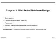
Set Query Benchmark KNK columns 

K5 has 5 values, each appearing randomly on about 200,000 rows 

4 

1 

5 

3 

4 

2 

5 

1 

… 

K5=3 on 1/5 of 

the rows,so we 

say FF = 1/5 

for K5=3 

K10K has 10,000 values, each appearing 

randomly on about 100 rows 

3457 

0003 

5790 

0123 

4523 

… 

K10K=3 on 

1/10000 of the 

rows,so its FF 

= 1/10000

DB Performance: Set Query Benchmark 

 

Here is an example of Query Suite Q3B (underline: fix handout) 

SELECT SUM(K1K) FROM BENCH 

WHERE (KSEQ between 400000 and 410000 OR KSEQ between 420000 and 430000 

OR KSEQ between 440000 and 450000 OR KSEQ between 460000 and 470000 

OR KSEQ between 480000 and 500000) AND KN = 3; -- KN varies from K5 to K100K 

---------------------------|==|---|==|---|==|---|==|---|==|==|--------------------------------------------------------- 

KSEQ-> 400000 500000 (midpoint in KSEQ) 

 

 

 

 

This query sums dollar sales of a product of varying popularity 

sold in a given locale (thus in a broken range of zip codes) 

DB2 and M204 both ran on IBM mainframe system MVS; Note 

that the FF for KSEQ range is 0.06 and for KN = 3 is 1/CARD(KN) 

DB2 did very well on queries requiring sequential or skipsequential 

access to data (called sequential prefetch or listprefetch 

by DB2), useful in Q3B 

We wish to contrast performance in 1988-9 measurements of 

MVS DB2 vs 2007 measurements of DB2 UDB on Windows 

19

DB Performance: Set Query Comparison 

On Windows ran DB2 UDB on a 10,000,000 row BENCH table 

using very fast modern system (very cheap compared to 1990) 

Query Plans for UDB same as MVS for KN = K100K, K10K & K5, 

but different for KN = K100, K25 and K10 

Composite FF for N = K10K is 0.06*(1/10,000) = 0.000006, so 6 

rows retrieved from MVS’s 1M, 62 rows from UDB’s 10M 

KN Used 

In Q3B 

Rows Read 

(of 1M) 

DB2 MVS 

1M Rows 

Index usage 

DB2 UDB 

10M Rows 

Index usage 

DB2 MVS 

1M Rows 

Time secs 

K100K 1 K100 K100 1.4 0.7 

K10K 6 K10K K10K 2.4 3.1 

K100 597 K100, KSEQ KSEQ 14.9 2.1 

K25 2423 K25, KSEQ KSEQ 20.8 2.4 

K10 5959 K10, KSEQ KSEQ 31.4 2.3 

K5 12011 KSEQ KSEQ 49.1 2.1 

DB2 UDB 

10M Rows 

Time secs 

20

Set Query Benchmark KNK index example 

K10K has 10,000 values, each 

appearing on about 100 rows 

K10K 

3457 

0003 

5790 

0123 

4523 

… 

100 entries for 

key = 3 

K10K index : B-tree of entries 

(only leaf level shown) 

Key RID 

… 

… 

002 23548901 

003 56893467 

003 59856230 

003 64908876 

… 

004 45980456 

… 

…


 

 

 

For both DB2 MVS & DB2 UDB, Query Plan for KN = K100K & 

K10K is: access rows with KN = 3 & test KSEQ in proper ranges 

DB2 MVS had .0001*(.06)*1,000,000 = 6 rows accessed for 

K10K; DB2 UDB with 10,000,000 rows, had 62 rows accessed 

In these cases of very low selectivity, index driven access to 

individual rows is still the best Query Plan 

KN Used 

In Q3B 

Rows Read 

(of 1M) 

DB2 MVS 

Index usage 

DB2 UDB 

Index usage 

DB2 MVS 

Time secs 

K100K 1 K100 K100 1.4 0.7 

K10K 6 K10K K10K 2.4 3.1 

DB2 UDB 

Time secs 

22


 

 

For KN = K100, K25 and K10, DB2 MVS ANDED KSEQ and 

KN = 3 RID-lists, and accessed rows by RID to sum K1K values 

x x x x x x x x x x xx x x x x x x x x xx x x xx x x x 

|=====|———|=====|———|=====| ———|=====| ———|==========| 

DB2 UDB on the other hand, scans each of five KSEQ ranges 

specified & tests KN = 3 before summing K1K; DB2 MVS and 

DB2 UDB both use that same plan for K5 

Scan&Tst Scan&Tst Scan&Tst Scan&Tst Scan and Test 

|=====|———|=====| ———|=====| ———|=====| ———|==========| 

KN Used 

In Q3B 

Rows Read 

(of 1M) 

DB2 MVS 

Index usage 

DB2 UDB 

Index usage 

DB2 MVS 

Time secs 

K100 597 K100, KSEQ KSEQ 14.9 2.1 

K25 2423 K25, KSEQ KSEQ 20.8 2.4 

K10 5959 K10, KSEQ KSEQ 31.4 2.3 

K5 12011 KSEQ KSEQ 49.1 2.1 

DB2 UDB 

Time secs 

23


 

 

 

Both indexed retrieval of individual rows and sequential scan 

have sped up since DB2 MVS, but sequential scan much more! 

Sequential scan speed has increased from MVS to UDB by a 

factor of 88; random row retrieval speed by a factor of 4 

FFs for speeding up random row retrieval are less important, but 

clustering is more important: reduces sequential scan range 

KN Used 

In Q3B 

Rows Read 

(of 1M) 

DB2 MVS 

Index usage 

DB2 UDB 

Index usage 

DB2 MVS 

Time secs 

K100K 1 K100 K100 1.4 0.7 

K10K 6 K10K K10K 2.4 3.1 

K100 597 K100, KSEQ KSEQ 14.9 2.1 

K25 2423 K25, KSEQ KSEQ 20.8 2.4 

K10 5959 K10, KSEQ KSEQ 31.4 2.3 

K5 12011 KSEQ KSEQ 49.1 2.1 

DB2 UDB 

Time secs 

24

Disk Performance 

 

 

 

 

Our “disktest” program generates read requests to a 20 GB file, 

as a database would 

Sits on 4-disk RAID system of enterprise disks (15K RPM) 

Various read request sizes: rsize = 4KB, 16KB, 64KB, 256KB 

From 1 to 300 read requests outstanding 

Either read whole file in order in rsize reads, or only some of 

it: “skip-sequential” reads 

We use random numbers to determine successive rsize 

blocks to read, with probability p, p = 1.0, 0.1, 0.01, 0.001 

Case of p = 1.0 specifies sequential reading, like a table scan 

Case of p < 1.0 specifies skip-sequential, like index-driven 

database access: ordered RIDs access rows left-to-right on disk 

DB2 orders RIDs before accessing, ORACLE seems not to 

25

Disk Performance 

 

 

 

Rectangles in disks above represent requests queued in each individual 

disk of a RAID set with multiple requests outstanding (SCSI or SATA) 

Each disk runs the “elevator” algorithm, modified to handle rotational 

position, to optimize its work 

For skip-sequential reading, we need 20 requests outstanding for good 

performance, 5 in each disk 

This is 3-5 times faster than with 1 request outstanding 

But not highest MB/s: disk has to rotate between reads 

Note: stripe size doesn’t matter here, as long as multiple stripes of 

data are in play 

26

Sequential Scan Performance 

 

 

 

 

 

 

Each disk can deliver 100MB/second with sequential scan 

But throughput from disk to memory is limited by controller/bus 

Disktest, reading sequentially, gets a maximum of 300MB/sec 

 

 

 

 

 

Need reads aligned to stripe boundaries to achieve maximum 300MB/sec 

Our 4-disk RAID has 64KB stripe size, the Windows page I/O size 

With 256KB reads (4 disk stripe set), only need 2 requests outstanding for 

300MB/sec 

64KB reads (1 disk stripe at a time), 20 requests outstanding for 300MB/sec 

Maximum read speed is not attainable with 4KB or 16KB reads 

DBs get about 140 MB/second using tablescan (after tuning) 

 

Slowed down by needing to interpret data read in, extract rows, etc. 

Need to tune DBs to use large reads, multiple outstanding reads 

Oracle and Vertica recommend 1MB stripe size for DB RAID 

27

Pointers on Setting up disks for DBs 

 

 

 

 

 

 

 

When experimenting, should partition RAID into (say) 5 parts 

Then can save tuned databases on different partitions 

Can reinitialize file system on old partition and copy data from 

another; avoids file system fragmentation of multiple loads 

Can also build a new database on reinitialized partition 

Don’t worry about “raw disk”: current OS file I/O is great 

You will find that the lower-numbered partitions have faster 

sequential reads, because of disk “zones” 

effect is about 30% for enterprise disks, more for cheap disks 

Just be aware of this effect, so you don’t misinterpret results 

You can buy enterprise disks to use on an ordinary tower PC 

We used a Dell PowerEdge 2900, nice accessible internals 

Added SAS RAID controller, SAS disks 

28

DB Performance:Outline of What Follows 

First, we’ll examine Clustering historically, then a new 

DB2 concept of Multi-Dimensional Clustering (MDC) 

We show how a form of MDC can be applied to other 

DBMS products as well, e.g., Oracle, Sybase IQ 

We want to apply this capability in the case of Star 

Schema Data Warehousing, but there’s a problem 

We explain Star Schemas, and how the problem can 

be addressed by Adjoined Dimension Columns 

We introduce a “Star Schema Benchmark” and show 

performance comparisons of three products 

29

DB Performance: Linear Clustering 

 

 

 

 

 

 

Indexed clustering is an old idea; in 1980s one company had 

demographic data on 80 million families from warranty cards 

They crafted mail lists for sales promotions of client companies 

Typically, they concentrated on local areas (store localities) for 

these companies to announce targeted sales: sports, toys, etc. 

To speed searches, they kept families in order by zipcode; also 

had other data, so could restrict by incomeclass, hobbies, etc. 

The result was something like like Q3B: a 50 mile radius circle in 

a state will result in a small union of ranges on zipcode 

The Q3B range union was a fraction 0.06 of all possible values 

in clustering column KSEQ in BENCH 

Clustered ranges are all the more important with modern disks 

30

Multi-Dimensional Clustering 

Clustering by a single column of a table is fine if almost all 

queries restrict by that column, but this is not always true 

DB2 was the first DBMS to provide a means of clustering by 

more than one column at a time using MDC 1 

MDC partitions table data into Cells by treating some columns 

within the table as axes of a Cube 

Each Cell in a Cube is defined by a combination of values in 

Cube axis columns: Each row’s axis values define its Cell 

New rows are placed in its Cell, which sits on a sequence of 

Blocks on disk; Blocks must be large enough so sequential scan 

access speed on the cell swamps inter-cell access seek 

Queries with multiple range predicates on axis columns will 

retrieve only data from Cells in range intersection 

1 S. Lightstone, T. Teory and T. Nadeau. Physical Database Design. Morgan Kaufmann 

31

DB Performance: Multi-Dim Clustering 

Example cube on dimensions: Year, Nation, Product Category 

Year 

Category 

Nation 

32


 

 

 

 

 

 

Define DB2 MDC Cells in Create Table statement 

create table Sales(units int, dollars decimal(9.2), prodid int, category int, nation 

char(12), selldate date, year smallint, . . .) 

organize by dimensions (category, nation, year); 

Cells on category, nation and year are created, sit on blocks 

Each value of a dimension gives a Slice of the multi-dimensional 

cube; has Block index entry listing BIDs of Blocks with that value 

The BIDs in the intersection of all orthogonal Slices is for a Cell 

DB2 supports Inserts of new rows of a table in MDC form; new 

rows are placed in some Block of the valid Cell, with new Block 

added if necessary; after Deletes, empty Blocks are freed 

No guarantee Blocks for a Cell are near each other, but interblock 

time swamped by speed of sequentially access to a block 

33

MDC organization on disk 

Example: MDC with three axes (AKA dimensions), nation, 

year, category, each with values 1, 2, 3, 4. 

Let C123 stand for cell with axis values (1,2,3), I.e., nation = 

1, year = 2, category = 3 

On disk, each block (1 MB say) belongs to a cell. 

The sequence of blocks on disk is disordered: 

C321 C411 C342 C433 C412 C143 C411 C231 C112 … 

One cell, say C411, (nation = 4, year = 1, category = 1) has 

several blocks,in different places, but since each block is 1 

MB, it’s worth a seek.

DB Performance: Star Schema (SS) 

 

 

A Data Warehouse is a Query-mostly Database, typically made 

up of multiple Star Schemas, called Data Marts 

Star Schema has Fact table and various Dimension tables 

Date Dimension 

Date Key (PK) 

Many Attributes 

Store Dimension 

Store Key (PK) 


POS Transaction Fact 

Date Key (FK) 

Product Key (FK) 

Store Key (FK) 

Promotion Key (FK) 

Transaction Number 

Sales Quantity 

Sales Dollars 

Cost Dollars 

Profit Dollars 

Product Dimension 

Product Key (PK) 


Promotion Dimension 

Promotion Key (PK) 


35

DB Performance: Star Schema (SS) 

 

 

 

 

 

In general, Dimension tables have a very small number of rows 

compared to a Fact table 

POS Transaction Fact Table has 9 columns, 40 byte rows 

Maximum size of a POS table on an inexpensive PC might need 

a few hundred GB of disk, which would amount to 5 billion rows 

Dimension tables are much smaller: few thousand rows in Date, 

Store Dimensions, 100s in Promotion, few million in Product 

Practitioners keep Fact tables lean,Foreign Keys, TID and 

Measures, have many descriptive columns in Dimension Tables 

E.g. Product Dimension might have: ProdKey (artificial key), 

Product Name, SKU (natural key), Brand_Name, Category 

(paper product), Department (sporting goods), Package_Type, 

Package _Size, etc 

36

DB Performance: Data Warehousing 

 

Data Warehouse is made up of collection of Star Schemas often 

representing supply chain on conforming dimensions 1 

1 R. Kimball & M. Ross, The Data Warehouse Toolkit, 2nd Ed., Wiley 

CONFORMING DIMENSIONS 

SUPPLY CHAIN STAR SCHEMAS 

Date 

Product 

Store 

Promotion 

Warehouse 

Vendor 

Contract 

Shipper 

Etc. 

Retail Sales X X X X 

Retail Inventory X X X 

Retail Deliveries X X X 

Warehouse Inventory X X X X 

Warehouse Deliveries X X X X 

Purchase Orders X X X X X X 

37

DB Performance: Star Schema Queries 

 

 

 

 

Queries on Star Schemas typically retrieve aggregates of Fact 

table measures (Sales Quantity/Dollars/Cost/Profit) 

The Query Where Clauses typically restrict Dimension Columns: 

Product Category, Store Region, Month, etc. 

Usually some Group By for Aggregation 

Example Query 2.1 from Star Schema Benchmark (SSB): 

select sum(lo_revenue), d_year, p_brand1 

from lineorder, date, part, supplier 

where lo_orderdate = d_datekey and lo_partkey = p_partkey 

and lo_suppkey = s_suppkey and p_category = 'MFGR#12' 

and s_region = 'AMERICA' 

group by d_year, p_brand1 order by d_year, p_brand1; 

38


 

 

 

 

 

 

Recall that DB2’s MDC treats table columns as orthogonal axes 

of a Cube; these columns are called “Dimensions” 

But MDC “Dimensions” are columns in a table turned into a 

Cube, not columns in Dimension tables of a Star Schema 

Of course we can’t embed all Dimension columns of a Star 

Schema in the Fact table: would take up too much space for 

huge number of rows 

How does DB2 MDC handle Star Schemas? Not entirely clear 

For a foreign key of type Date a user can define a “generated 

column” YearAndMonth mapped from Date by DB2; this 

column’s values can then be used to define MDC Cells 

But not all Dimension columns can have generated columns 

defined on foreign keys: Product foreign key will not give brand 

39

Adjoined Dimension Columns (ADC) 

 

 

 

 

 

 

To use columns of Star Schema Dimension tables in MDC as 

Cube Axes we adjoin copies of Dimension columns to Fact table 

We call this “ADC”: Adjoined Dimension Columns for Cube Axes 

Only 3-5 columns adjoined of relatively low cardinality, since the 

number of Cells is the product of table Axis column values 

Why is low cardinality important? 

Each Cell (or Block of a Cell) must sit on a MB of disk or more, 

so sequential access in Cell swamps seek time between Cells 

(DB2 MDC documents don’t describe this, but that’s the idea) 

The ADC approach generalizes to DBMS without MDC if we sort 

Fact table by concatenation of adjoined columns 

We explain all this and measure performance in what follows 

40

ADC: Outline of What Follows 

ADC works well with DB2 MDC or Oracle partitions or 

even a DBMS that simply has good indexing 

ADC can have problems with inserts to the base table 

if Cells are not defined on a Materialized View 

We will measure performance using a Star Schema 

benchmark (SSB): The SSB schema is defined as a 

transformation of a TPC-H benchmark schema 

We analyze SSB Queries by clustering performed: 

Cluster Factor (CF) instead of Filter Factor (FF) 

Then we provide experimental results, further 

analysis, and conclusions 

41

Adjoining Dimension Columns: Example 

Consider adjoining the following dimension columns to the POS 

Transaction Fact table (Slide pg 27) to give POS ADC 

Date.Qtr in a 3 year history of transactions, 12 values, as POS.D_Qtr 

Store.Nation in multi-national sales with 9 nations, as POS.S_Nation 

Product.Dept, with 18 Departments in the business, POS.P_Dept 

Promotion.MediaType, with 9 such types, as POS.PR_Type 

Number of cells added to make POS ADC is: 12*9*18*9 = 17,496 

May see skew in count of rows in cell combinations of dimension 

column values: say smallest cells size is 1/2 size of largest 

We want each cell to contain at least 1 MB so sequential scan 

swamps seek time between cells: We should be safe assuming 

35000 cells of equal size: implies we need 70 GB in POS ADC 

42

Considerations and Futures of ADC 

If POS ADC is not a materialized view, updates don’t keep POS up 

to date: may be OK if it’s only POS ADC we want to work with 

POS ADC isn’t much fatter than POS, four extra columns with small 

cardinality: can make these columns tiny with good compression 

E.g., character string values can EACH be mapped to small ints 

1-12; this approach was used in M204: “Coding” compression 

POS ADC Inserts might be slow if must look up ADC in Dimensions 

But it seems possible to encode column values of a dimension 

hierarchy in a hierarchical foreign key: Region (4 values), Nation 

(up to 25 per region), City (up to 25 per Nation): 2 + 5 + 5 bits. 

An added advantage is that the DBMS becomes hierarchy aware 

with just a foreign key: can recognize that an equal match on City 

implies equal match on containing Country and Region 

This obviates the needs to put “hints” in query of Country/Region 

44

Compressing ADC 

Won’t have all tricks of prior slide in any current DBMS 

But we can usually compress adjoined dimension columns to 

small ints: use UDF for mapping so Store.Nation = ‘United 

States’ maps to small int 7 

create function NATcode (nat char(18)) returns small int 

… 

return case nat 

when ‘United Kingdom’ then 1 

… 

when ‘United States’ then 7 

… 

end 

Now a user can write: 

Select … from POS where S_Nation = Natcode(‘United States’)… 

Natcode will translate ‘United States’ to the int 7; thus all ADC 

can be two-byte (or less) small ints with proper UDFs defined 

45

Using ADC With Oracle 

Oracle has a feature “Partitioning” that corresponds to DB2 MDC 

Given ADCs C1, C2, C3 and C4, create Cells of a Cube using the 

Partition clause in Create Table on a concatenation of these 

columns (assume values for columns are 0, 1 & 2, for illustration) 

… 

partition C0001 values less than (0,0,0,1) tablespace TS1 


partition C0010 values less than (0,0,1,0) tablespace TS1 -- (0,0,1,0) next after (0,0,0,2) 

… 


… 

-- NOTE: Inserts of new rows also work with partitioning 

Map Dimension value to number, Oracle compresses to byte if fits 

create or replace function natcode (nat char(18)) return number is 

begin 

return case nat 

when ‘United Kingdom’ then 1 

… 

46

Create Cells Using Table Order & ADC 

For DBMS with good indexing, define Cells by concatenating (4) 

Adjoined Dimension Columns and sorting table by this order 

Each cell represents unique combination of ADC values (2,7,4,3) 

 

 

 

 

A Where clause with ANDed range predicates on four ADCs, each range 

over 3 ADC values, will select 81 cells on the table 

Cells Selected will not sit close to each other, except for cells differing 

only in the final ADC values, e.g.: (2,7,4,3) and (2,7,4,4) 

Obviously this approach doesn’t allow later inserts into given cells 

The Vertica DBMS uses this approach, but since new inserts go into 

WOS in memory, later merged out to disk ROS, new ad hoc inserts ARE 

possible 

47

Star Schema Benchmark (SSB) 

Recall: Kimball defines a Data Warehouse made up Data Marts 

represented by Star Schemas on conforming dimensions (pg 27) 

To measure query performance on a Star Schema Data Mart with 

and without ADC, we define the Star Schema Benchmark (SSB) 1 

The SSB design is based on that of the TPC-H benchmark 2 , used 

by many vendors to claim superior Data Warehouse performance 

“[TPC-H] is cleverly constructed to avoid using a Snowflake [Star] 

Schema; [two dozen CIOs have] never seen a data warehouse 

that did not use a Snowflake schema” 3 

We base SSB on TPC-H for data warehouse needs; Note TPC 

has been trying for years to develop a Star Schema benchmark 

1 P. O’Neil, E. O’Neil, X. Chen. The Star Schema Benchmark. 

http://www.cs.umb.edu/~poneil/StarSchemaB.PDF 

2 TPC-H, an ad-hoc decision support benchmark. http://www.tpc.org/tpch/ 

3 M. Stonebraker et al., One Size Fits All? — Part 2: Benchmarking Results. http://wwwdb.cs.wisc.edu/cidr/cidr2007/index.html, 

press ‘Electronic Proceedings’ to download 

48

Star Schema Benchmark (SSB) 

Created to Measure Star Schema Query Performance 

49

SSB is Derived From TPC-H Benchmark 

PART (P_) 

SF*200,000 

PARTKEY 

PARTSUPP (PS_) 

SF*800,000 

PARTKEY 

LINEITEM (L_) 

SF*6,000,000 

ORDERKEY 

ORDERS (O_) 

SF*1,500,000 

ORDERKEY 

NAME 

SUPPKEY 

PARTKEY 

CUSTKEY 

MFGR 

AVAILQTY 

SUPPKEY 

ORDERSTATUS 

BRAND 

SUPPLYCOST 

LINENUMBER 

TOTALPRICE 

TYPE 

COMMENT 

QUANTITY 

ORDERDATE 

SIZE 

CONTAINER 

RETAILPRICE 

COMMENT 

SUPPLIER (S_) 

SF*10,000 

SUPPKEY 

NAME 

ADDRESS 

NATIONKEY 

PHONE 

ACCTBAL 

CUSTOMER (C_) 

SF*150,000 

CUSTKEY 

NAME 

ADDRESS 

NATIONKEY 

PHONE 

ACCTBAL 

MKTSEGMENT 

COMMENT 

NATION (N_) 

25 

NATIONKEY 

EXTENDED- 

PRICE 

DISCOUNT 

TAX 

RETURNFLAG 

LINESTATUS 

SHIPDATE 

COMMITDATE 

RECEIPTDATE 

SHIPINSTRUCT 

SHIPMODE 

COMMENT 

ORDER- 

PRIORITY 

CLERK 

SHIP- 

PRIORITY 

COMMENT 

COMMENT 

NAME 

REGIONKEY 

REGION (R_) 

5 

REGIONKEY 

COMMENT 

NAME 

COMMENT 

50

Why Changes to TPC-H Make Sense 

TPC-H has PARTSUPP table listing Suppliers of ordered Parts to 

provide information on SUPPLYCOST and AVAILQTY 

This is silly: there are seven years of orders (broken into ORDERS 

and LINEITEM table) and SUPPLYCOST not stable for that period 

PARTSUPP looks like OLTP, not a Query table: as I fill orders I 

would want to know AVAILQTY, but meaningless over 7 years? 

AVAILQTY and SUPPLYCOST are never Refressed in TPC-H 

either; We say PARTSUPP has the wrong temporal “granularity” 1 

One suspects the real reason for PARTSUPP is to break up what 

would be a Star Schema, so Query Plans become harder 

Combining LINEITEM and ORDER in TPC-H to get LINEORDER in 

SSB, with one row for each one in LINEITEM, is common practice 1 

1 

The Data Warehouse Toolkit, 2nd Ed, Ralph Kimball and Margy Ross. Wiley 

51

Why Changes to TPC-H Make Sense 

To take the place of PARTSUPP, we have a column SUPPLYCOST 

in LINEORDER of SSB to give cost of each item when ordered 

Note that a part order might be broken into two or more lineitems 

of the order if lowest cost supplier didn’t have enough parts 

Another modification of TPC-H for SSB was that TPC-H columns 

SHIPDATE, RECEIPTDATE and RETURNFLAG were all dropped 

This information isn’t known until long after the order is placed; 

we kept ORDERDATE and COMMITDATE (the commit date is a 

commitment made at order time as to when shipment will occur) 

One would typically need multiple star schemas to contain other 

dates from TPC-H, and we didn’t want SSB that complicated 

A number of other modifications were made; for a complete list, 

see: http://www.cs.umb.edu/~poneil/StarSchemaB.PDF 

52

Star Schema Benchmark Queries 

SSB has 13 queries of TPC-H form, with varying numbers of dimension 

columns restricted & varying selectivity of restrictions; examples follow 

Q1.1: Select the total discount given in 1993 for parts sold in quantity < 25 

and with discounts of 1-3% 

select sum(lo_extendedprice*lo_discount) as revenue 

from lineorder, date 

where lo_orderdate = d_datekey and d_year = 1993 

and lo_discount between1 and 3 and lo_quantity < 25; 

Q2.1: Measure total revenue for a given part category from a supplier in a certain 

geographical area 

select sum(lo_revenue), d_year, p_brand1 

from lineorder, date, part, supplier 

where lo_orderdate = d_datekey and lo_partkey = p_partkey and lo_suppkey 

= s_suppkey and p_category = 'MFGR#12’ and s_region = 'AMERICA' 

group by d_year, p_brand1 order by d_year, p_brand1; 

53

Star Schema Benchmark Queries 

Successive Queries in a flight (Q1.2, Q1.3 in flight Q1) use tighter 

restrictions to reduce Where clause selectivity 

Q1.1:Select the total discount given in 1993 for parts sold in quantity < 25 

and with discounts of 1-3% 



where lo_orderdate = d_datekey and d_year = 1993 

and lo_discount between1 and 3 and lo_quantity < 25; 

Q1.3: Same as Q1.1, except parts sold in smaller range and date limited to 

one week 



where lo_orderdate = d_datekey and d_weeknuminyear = 6 and d. year = 1994 

and lo_discount between 5 and 7 and lo_quantity between 25 and 35 

See list of queries starting on page 9 of ADC Index preprint handout 

54

Star Schema Benchmark Cluster Factors 

Query 

CF on 

lineorder 

CF on 

discount 

& quantity 

CF on 

Date 

CFs of indexable predicates 

on dimension columns 

CF on CF on CF on 

part supplier customer 

Brand1 city roll-up city rollup 

roll-up 

Combined CF Effect 

on lineorder 

Q1.1 .47*3/11 1/7 .019 

Q1.2 .2*3/11 1/84 .00065 

Q1.3 .1*3/11 1/364 .000075 

Q2.1 1/25 1/5 1/125 = .0080 

Q2.2 1/125 1/5 1/625 = .0016 

Q2.3 1/1000 1/5 1/5000 = .00020 

Q3.1 6/7 1/5 1/5 6/175 = .034 

Q3.2 6/7 1/25 1/25 6/4375 = .0014 

Q3.3 6/7 1/125 1/125 6/109375 =.000055 

Q3.4 1/84 1/125 1/125 1/1312500= .000000762 

Q4.1 2/5 1/5 1/5 2/125 = .016 

Q4.2 2/7 2/5 1/5 1/5 4/875 = .0046 

Q4.3 2/7 1/25 1/25 1/5 2/21875 = .000091 

55

SSB Test Specifications 

We measured three DB products we call A, B, and C, using SSB 

tables at Scale Factor 10, where LINEORDER has about 6 GB 

Tests were performed on a Dell 2900 running Windows Server 

2003, with 8 GB of RAM (all queries had cold starts), two 64-bit 

dual core processors (3.2 GHz each), and data loaded on RAID0 

with 4 Seagate 15000 RPM SAS disks (136 GB each), with stripe 

size 64 KB This is a fast system in current terms; 

We had to experiment to find good tuning settings for number of 

reads outstanding: parallel threads, prefetching 

Adjoined dimension columns were d.year, s.region, c.region, and 

p.category (brand-hierarchy), cardinalities 7, 5, 5, and 25 

In LINEORDER table these adjoined columns were named year, 

sregion, cregion, category, and used in the SSB Queries 

56

SSB Load 

 

 

 

We performed two loads for DBs A, B and C, one with adjoined columns 

and one with no adjoined columns, called BASIC form 

First we generated rows of SSB LINEORDER and dimensions using 

generator that populates TPC-H, with needed modifications 

After loading LINEORDER in Basic form, used a query (below) to output 

the data with adjoined columns in order by concatenation; could use this 

order to load DB with indexing, or to help speed up DB2 MDC load and 

Oracle Partition load 

select L.*, d_year, s_region, c_region, p_category 

from lineorder, customer, supplier, part, date 

where lo_custkey = c_custkey and lo_suppkey = s_suppkey 

and lo_partkey = p_partkey and lo_datekey = d_datekey 

order by d_year, s_region, c_region, p_category; 

57

DB Products A, B & C Times in Seconds 

58

A, B & C Geom. Mean of ADC Measures 

It’s clear that the queries of SSB are best optimized by a column 

store (also referred to as “vertically partitioned”), DB Product C 

Normal way to summarize N time measures is a geometric mean 

(used by TPC) : Nth root (Product of N measures) 

The assumption is that faster queries (smaller times) will be used 

more often, so all queries will have equal weight 

Here are Geometric Means of elapsed & CPU times for A,B,C 

Product A 

(row DB) 

Base Case 

Product B 

(row DB) 

Base Case 

Product C 

(Col, DB) 

Base Case 

Product A 

(row DB) 

ADC Case 

Product B 

(row DB) 

ADC Case 

Product C 

(Col, DB) 

ADC Case 

Geometric 

Mean of 

Elapsed/CPU 

Seconds 

44.7/3.4 36.8/1.5 12.6/1.6 3.60/0.24 4.23/0.236 2.29/0.0081 

59

Analysis of SSB and Conclusions 

Query Times vs. Cluster Factor, CF (on log scale) 

60

Analysis of SSB and Conclusions 

 

 

 

 

 

On plot of slide 56, differentiate three regions of cluster factor: CF 

At low end of the CF Axis (CF < 1/10000), secondary indexes are 

effective at retrieving few rows qualified: ADC has little advantage 

For CF up near 1.0, the whole table is read with sequential scan 

regardless of ADC, and the times again group together 

For CF in the intermediate range where most queries lie, ADC reduces 

query times very effectively compared to the BASE case 

Time is reduced from approximately that required for a sequential scan 

down to a few seconds (at most ten seconds) 

We believe this demonstrates the validity of our ADC approach 

61

Analysis and Conclusions 

 

 

 

 

Readers should bear in mind that the Star Schema Benchmark has quite 

small dimensions, with rather simple rollup hierarchies 

With more complex dimensions and query workloads in large 

commercial applications, no single ADC choice will speed up all possible 

queries 

Of course this has always been the case with clustering solutions: they 

never improve performance of all possible queries 

Still, there are many commercial data warehouse applications where 

clustering of this sort should be an invaluable aid 

62

Bibliography 

H. Berenson, P Bernstein, J. Gray, J. Melton, P. O’Neil, E. O’Neil, A Critique of 

ANSI Isolation Levels. SIGMOD 2005. 

D. Chamberlin and R. Boyce, SEQUEL: A Structured English Query Language. 

SIGFIDET 1974 (later SIGMOD), pp. 249-264. 

A. Fekete, D. Liarokapis, E. O’Neil, P. O’Neil and D. Shasha. Making Snapshot 

Isolation Serializable. ACM TODS, Vol 30, No. 2, June 2005 

Jim Gray, ed., The Benchmark Handbook, in ACM SIGMOD Anthology, 

http://www.sigmod.org/dblp/db/books/collections/gray93.html 

R. Kimball & M. Ross, The Data Warehouse Toolkit, 2nd Ed., Wiley, 2002 

S. Lightstone, T. Teory and T. Nadeau. Physical Database Design, Morgan 

Kaufmann, 2007 

P. O’Neil, E. O’Neil, X. Chen. The Star Schema Benchmark. 

http://www.cs.umb.edu/~poneil/StarSchemaB.PDF 

63

Bibliography 

P.G. Selinger et al., Access Path Selection in a relational database 

management system. SIGMOD 1979; 

M. Stonebraker et al, C-Store, A Column-Oriented DBMS, VLDB 2005. 

http://db.csail.mit.edu/projects/cstore/vldb.pdf 

M. Stonebraker et al., One Size Fits All? — Part 2: Benchmarking Results. 

CIDR 2007 http://www-cs.wisc.edu/cidr/cidr2007/index.html, press 

‘Electronic Proceedings’ to download 

TPC-H, an ad-hoc decision support benchmark. http://www.tpc.org/tpch/ 

64

Tutorial slides

Create successful ePaper yourself

Delete template?

Save as template?