Correlated Multi-Jittered Sampling - Pixar Graphics Technologies
Correlated Multi-Jittered Sampling - Pixar Graphics Technologies
Correlated Multi-Jittered Sampling - Pixar Graphics Technologies

Create successful ePaper yourself
Turn your PDF publications into a flip-book with our unique Google optimized e-Paper software.
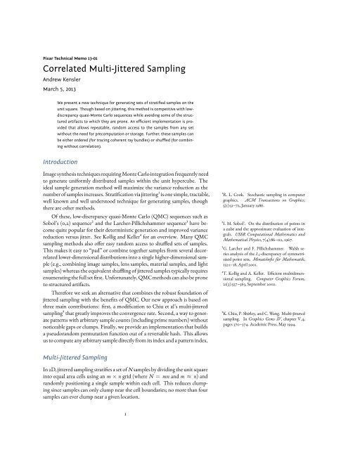
<strong>Pixar</strong> Technical Memo 13-01<br />
<strong>Correlated</strong> <strong>Multi</strong>-<strong>Jittered</strong> <strong>Sampling</strong><br />
Andrew Kensler<br />
March 5, 2013<br />
We present a new technique for generating sets of stratified samples on the<br />
unit square. Though based on jittering, this method is competitive with lowdiscrepancy<br />
quasi-Monte Carlo sequences while avoiding some of the structured<br />
artifacts to which they are prone. An efficient implementation is provided<br />
that allows repeatable, random access to the samples from any set<br />
without the need for precomputation or storage. Further, these samples can<br />
be either ordered (for tracing coherent ray bundles) or shuffled (for combining<br />
without correlation).<br />
Introduction<br />
Image synthesis techniques requiring Monte Carlo integration frequently need<br />
to generate uniformly distributed samples within the unit hypercube. The<br />
ideal sample generation method will maximize the variance reduction as the<br />
number of samples increases. Stratication via jittering is one simple, tractable,<br />
well known and well understood technique for generating samples, though<br />
there are other methods.<br />
Of these, low-discrepancy quasi-Monte Carlo (QMC) sequences such as<br />
Sobol’s (0,2) sequence and the Larcher-Pillichshammer sequence have become<br />
quite popular for their deterministic generation and improved variance<br />
reduction versus jitter. See Kollig and Keller for an overview. Many QMC<br />
sampling methods also oer easy random access to shued sets of samples.<br />
This makes it easy to “pad” or combine together samples from several decorrelated<br />
lower-dimensional distributions into a single higher-dimensional sample<br />
(e.g., combining image samples, lens samples, material samples, and light<br />
samples) whereas the equivalent shuing of jittered samples typically requires<br />
enumerating the full set rst. Unfortunately, QMC methods can also be prone<br />
to structured artifacts.<br />
Therefore we seek an alternative that combines the robust foundation of<br />
jittered sampling with the benets of QMC. Our new approach is based on<br />
three main contributions: rst, a modication to Chiu et al’s multi-jittered<br />
sampling that greatly improves the convergence rate. Second, a way to generate<br />
patterns with arbitrary sample counts (including prime numbers) without<br />
noticeable gaps or clumps. Finally, we provide an implementation that builds<br />
a pseudorandom permutation function out of a reversable hash. This allows<br />
us to compute any arbitrary sample directly from its index and a pattern index.<br />
R. L. Cook. Stochastic sampling in computer<br />
graphics. ACM Transactions on <strong>Graphics</strong>,<br />
5(1):51–72, January 1986.<br />
I. M. Sobol’. On the distribution of points in<br />
a cube and the approximate evaluation of integrals.<br />
USSR Computational Mathematics and<br />
Mathematical Physics, 7(4):86–112, 1967.<br />
G. Larcher and F. Pillichshammer. Walsh series<br />
analysis of the L -discrepancy of symmetrisized<br />
point sets. Monatshee für Mathematik,<br />
132:1–18, April 2001.<br />
T. Kollig and A. Keller. Ecient multidimensional<br />
sampling. Computer <strong>Graphics</strong> Forum,<br />
21(3):557–563, September 2002.<br />
K. Chiu, P. Shirley, and C. Wang. <strong>Multi</strong>-jittered<br />
sampling. In <strong>Graphics</strong> Gems IV, chapter V.4,<br />
pages 370–374. Academic Press, May 1994.<br />
<strong>Multi</strong>-<strong>Jittered</strong> <strong>Sampling</strong><br />
In 2D, jittered sampling straties a set of N samples by dividing the unit square<br />
into equal area cells using an m × n grid (where N = mn and m ≈ n) and<br />
randomly positioning a single sample within each cell. This reduces clumping<br />
since samples can only clump near the cell boundaries; no more than four<br />
samples can ever clump near a given location.<br />
1
However, jittering suers when these samples are projected onto the X- or<br />
Y-axis. In this case, we eectively have only m or n strata rather than N. This<br />
can greatly increase the variance at edges, especially when they are nearly axisaligned.<br />
The N-rooks sampling pattern xes this by jittering independently in<br />
each dimension, shuing the samples from one of the dimensions, and then<br />
pairing the samples from each dimension. This gives the full N strata when<br />
projecting onto an axis, but may result in more clumping in 2D.<br />
Chiu et al’s multi-jittered sample pattern achieves both of these properties<br />
simultaneously. Each cell and each horizontal or vertical substratum is occupied<br />
by a single jittered sample. Their method for producing these samples<br />
begins by placing them in an ordered, “canonical” arrangement as shown in<br />
Figure 1:<br />
P. Shirley. Discrepancy as a quality measure for<br />
sample distributions. In Eurographics ’91, pages<br />
183–193, September 1991.<br />
Listing 1: Producing the canonical arrangement.<br />
for (int j = 0; j < n; ++j) {<br />
for (int i = 0; i < m; ++i) {<br />
p[j * m + i].x = (i + (j + drand48()) / n) / m;<br />
p[j * m + i].y = (j + (i + drand48()) / m) / n;<br />
}<br />
}<br />
The next step shues the arrangement. First, the X coordinates in each<br />
column of 2D cells are shued. Then, the Y coordinates in each row are shuf-<br />
ed:<br />
Figure 1: The canonical arrangement. Heavy<br />
lines show the boundaries of the 2D jitter cells.<br />
Light lines show the horizontal and vertical substrata<br />
of N-rooks sampling. Samples are jittered<br />
within the subcells.<br />
Listing 2: Shuing the canonical arrangement.<br />
for (int j = 0; j < n; ++j) {<br />
for (int i = 0; i < m; ++i) {<br />
<br />
int k = j + drand48() * (n - j);<br />
<br />
std::swap(p[j * m + i].x,<br />
<br />
p[k * m + i].x);<br />
}<br />
}<br />
for (int i = 0; i < m; ++i) {<br />
for (int j = 0; j < n; ++j) {<br />
<br />
int k = i + drand48() * (m - i);<br />
<br />
std::swap(p[j * m + i].y,<br />
<br />
p[j * m + k].y);<br />
}<br />
}<br />
Figure 2 shows an example of the result. The shue preserves the 2D jitter<br />
and the N-rooks properties of the original canonical arrangement. The result<br />
is slightly better than plain jitter, but still shows a degree of clumpiness and<br />
unevenness in the distribution of samples.<br />
<strong>Correlated</strong> <strong>Multi</strong>-<strong>Jittered</strong> <strong>Sampling</strong><br />
Figure 2: A multi-jittered sampling pattern.<br />
Our key observation is that a small tweak to the shuing strategy can make a<br />
dramatic improvement to the sample distribution: apply the same shue to<br />
the X coordinates in each column, and apply the same shue to the Y coordinates<br />
in each row. Listing 2 can be trivially changed to accomplish this simply<br />
by exchanging line 2 with 3, and line 9 with 10.<br />
This change greatly reduces the clumpiness as shown by the example pattern<br />
in Figure 3. There is a still a randomness to the position of the samples<br />
but they are much more evenly distributed throughout the unit square. The<br />
correlation in the shues means that each sample is now roughly /m apart<br />
2<br />
Figure 3: With correlated shuing.
horizontally from its neighbors to the le and right in the 2D jitter cells and /n<br />
apart vertically from its top and bottom neighbors (though they have greater<br />
lateral freedom in the relative placement). The only chance for clumping is<br />
from samples in diagonally connected jitter cells and because of the nature of<br />
the initial pattern and the special shuing, no more than two pairs of samples<br />
within a pattern may ever be in directly diagonally neighboring subcells. Note<br />
that these properties hold even under toroidal shis.<br />
If N is prime or otherwise not easily factored into m and n, there is a slight<br />
variation on the above algorithm that works very well. Choose m and n by<br />
rounding up such that N ≤ mn but they are otherwise as close to equal as<br />
possible. Then stretch the pattern along one axis by mn/N and clip the last<br />
mn − N samples (which should now be outside the unit square) from the<br />
end. This is illustrated in Figure 4. The remaining samples are evenly spaced<br />
along the stretched axis. Though this produces gaps in the substrata along the<br />
other axis, they will tend to be well distributed. It can also also result in minor<br />
clumping of the samples when wrapping the stretched axis toroidally.<br />
Figure 4: Irregular sample counts (N = in<br />
this example) by stretching and clipping.<br />
Results of <strong>Sampling</strong> on the Square<br />
Figure 5 shows an example of correlated multi-jittered sampling in use in a direct<br />
lighting test. Here, it compares favorably to jittered and QMC techniques<br />
for sampling an area light source; it is less noisy than the standard jittered sampling<br />
and avoids the structured artifacts seen with the Larcher-Pillichshammer<br />
sampling.<br />
Figure 5: <strong>Sampling</strong> a square area light. Rendered using 1 image sample and 25 light samples per pixel with per-pixel scrambling. The light-blockers are<br />
hidden to the camera. From top to bottom: standard jitter, Larcher-Pillichshammer, and correlated multi-jittered sampling.<br />
3
The cause of the artifacts for Larcher-Pillichshammer is shown in Figure 6;<br />
each sample falls at a regular /N interval along one axis (X in this case). This<br />
property is shared with Hammersley sampling and it is part of what gives them<br />
such low discrepancy. Presumably, adding jitter could help with this, albeit at<br />
the cost of increasing noise. Alternatively, instead of using per-pixel scrambling<br />
to produce a unique pattern at each pixel, some sampling patterns may<br />
be stretched over the entire image and used to produce all of the samples.<br />
This strategy can still alias, however (e.g., using the Halton sequence for image<br />
plane samples with an innite checkerboard plain scene). In general, lowdiscrepancy<br />
QMC sequences trade a higher potential for structured artifacts<br />
against faster convergence.<br />
The convergence rate of these and other sampling patterns in the above<br />
scene is shown in Figure 7. Here, variance is measured as the mean squared<br />
error relative to a reference image computed using 16384 jittered light samples<br />
per pixel. Above 25 samples per pixel, correlated multi-jittering generally outperforms<br />
all other methods except for the Larcher-Pillichshammer sequence.<br />
Figure 6: Larcher-Pillichshammer points. Light<br />
lines are at /N intervals.<br />
M. Pharr and G. Humphreys. Physically Based<br />
Rendering: From Theory To Implementation.<br />
Morgan Kaufmann, 2nd edition, 2010.<br />
10 -3 1 10 100 1000<br />
10 -4<br />
Uniform random<br />
<strong>Jittered</strong><br />
<strong>Multi</strong>-jittered<br />
Sobol's (0,2)<br />
<strong>Correlated</strong> multi-jittered<br />
Larcher-Pillichshammer<br />
10 -5<br />
Variance<br />
10 -6<br />
10 -7<br />
10 -8<br />
Samples per Pixel<br />
Figure 7: Samples per pixel versus variance in the above rectangular light source test scene.<br />
Similar measurements were done on scenes that tested other applications<br />
including the sampling of disk area lights, uniform- and cosine-weighted hemispheres<br />
for BRDFs, image plane positions for antialiasing, and lens positions<br />
for depth of eld. All showed the variance with correlated multi-jittering to<br />
be competitive with Sobol’s (0,2) sequence and occasionally competitive with<br />
the Larcher-Pillichshammer sequence. However, Sobol’s sequence has an advantage<br />
in that it does not require a bound on the number of samples to be<br />
known ahead of time and that it is hierarchical (i.e., the initial points in the<br />
sequence are well distributed) which can simplify progressive rendering.<br />
Table 1 shows the results of our nal evaluation method: for a number<br />
of dierent pattern generation algorithms, an example point set containing<br />
Pattern<br />
Discrepancy<br />
Uniform random .<br />
N-rooks<br />
.<br />
Poisson disk<br />
.<br />
<strong>Jittered</strong><br />
.<br />
<strong>Multi</strong>-jittered<br />
.<br />
Halton<br />
.<br />
Sobol’s (0,2)<br />
.<br />
<strong>Correlated</strong> multi-jittered .<br />
Hammersley<br />
.<br />
Larcher-Pillichshammer .<br />
Table 1: Patterns ordered by decreasing star discrepancy.<br />
4
1600 points on the unit square was generated and the star discrepancy was E. Thiémard. An algorithm to compute bounds<br />
estimated to within 0.0001. The relative ranking here corresponds well to the for the star discrepancy. Journal of Complexity,<br />
17(4):850–880, September 2001.<br />
ranking seen in Figure 7. In this test, correlated multi-jittered sampling had<br />
lower discrepancy than Halton and Sobol, the two hierarchical low-discrepancy<br />
sequences. Note that low discrepancy does not guarantee a good image however;<br />
the two lowest discrepancy patterns here are also the two most prone to<br />
the artifact seen in Figure 5.<br />
Results of <strong>Sampling</strong> on the Disk<br />
Because sampling disks and hemispheres are so crucial to BRDFs, we repeated<br />
the variance measurements using several methods for uniformly sampling a<br />
disk. The simplest of these approaches would be to assume that m ≈ n ≈<br />
√<br />
N as for sampling a square and then warp the samples from (x, y) in the<br />
square to polar coordinates on the disk with (θ, r) = (πx, √ y ). Figure 8<br />
shows an example of this. Note that the “seam” in the mapping is well hidden<br />
because the sample pattern wraps toroidally.<br />
A variation from Ward and Heckbert uses standard jittering with the same<br />
square-to-disk polar mapping, but chooses the number of 2D jitter cells so that<br />
m ≈ πn in order to stratify more strongly along the axis used for the angular<br />
component. This is perfectly doable with our correlated multi-jittering as well<br />
and an example of the result is shown in Figure 9.<br />
The last approach that we tested, illustrated in Figure 10, was to use the<br />
original m ≈ n ratio, but instead of the simple polar mapping we used Shirley<br />
and Chiu’s low distortion “concentric” disk mapping.<br />
Surprisingly, the simpler polar mapping consistently outperformed Shirley<br />
and Chiu’s mapping in terms of variance when used with our sampling algorithm.<br />
Of the two jitter stratication ratios, m ≈ n appeared to give slightly<br />
better results for sampling hemispheres (both uniformly and cosine weighted)<br />
while m ≈ πn was the slightly better ratio for so shadows from disk shaped<br />
area light sources. Note that the exact ratio is somewhat less relevant to correlated<br />
multi-jittering when compared to standard jittering due to the N-rooks<br />
property of the former; regardless of the actual ratio, the samples will be distributed<br />
into N strata when projected onto the X- or Y-axis. It is still important<br />
to maintaining the average 2D distance between the points, however.<br />
Figure 8: Polar warp with m = , n = .<br />
Heavy lines show the edges from the original<br />
unit square. Light lines show the boundaries of<br />
the 2D jitter cells.<br />
Figure 9: Polar warp with m = , n = .<br />
G. J. Ward and P. S. Heckbert. Irradiance gradients.<br />
In Third Eurographics Rendering Workshop,<br />
pages 85–98, May 1992.<br />
Pseudorandom Permutations<br />
The previously described method for generating correlated multi-jittered samples<br />
suces if we wish to generate all the samples in a given pattern at once.<br />
For practical reasons, however, we also want to be able to deterministically and<br />
repeatably compute an arbitrary sample out of the set of N in a given pattern.<br />
These samples may be needed in any order and some samples may never actually<br />
be needed.<br />
The diculty, then, arises mainly from the random shues on m or n<br />
elements at a time. As a shue is equivalent to indexing through a random<br />
permutation vector, we can reduce this to needing to eciently compute the<br />
element at position i in a random permutation vector of length l where the<br />
value p is used to select one of the l ! possible permutations.<br />
Interestingly, it turns out that this is a problem well studied in cryptography.<br />
For example, a 128-bit block cipher such as the Advanced Encryption<br />
Figure 10: “Concentric” disk mapping with m =<br />
, n = .<br />
P. Shirley and K. Chiu. A low distortion map<br />
between disk and square. Journal of <strong>Graphics</strong><br />
Tools, 2(3):45–52, 1997.<br />
5
Standard divides the plain text into 128-bit blocks and maps these through<br />
a permutation selected by bits from the key. It must be a permutation to be<br />
decryptable, and it must be statistically indistinguishable from a random permutation<br />
in order to be strong against an adversary.<br />
National Institute of Standards and Technology.<br />
Specication for the Advanced Encryption Standard<br />
(AES). Federal Information Processing<br />
Standards Publication (FIPS 197), 2001.<br />
Unfortunately, the domain of most block ciphers is much larger than we<br />
need. “Format preserving”, “data preserving”, or “small block” encryption attempts<br />
to address the need for smaller domains but can be quite expensive in<br />
time or space due to the need to withstand an adversary. Nonetheless, some<br />
of the concepts will prove useful.<br />
For a simpler, faster method we turn to hash functions. Several of the elementary<br />
functions used to create hash functions are reversible: B. Mulvey. Hash functions. http://home.<br />
comcast.net/~bretm/hash/, 2007.<br />
hash ^= constant;<br />
hash *= constant; // if constant is odd<br />
hash += constant;<br />
hash -= constant;<br />
hash ^= hash >> constant;<br />
hash ^= hash 1;<br />
w |= w >> 2;<br />
w |= w >> 4;<br />
w |= w >> 8;<br />
w |= w >> 16;<br />
do {<br />
i ^= p; i *= 0xe170893d;<br />
i ^= p >> 16;<br />
6
i ^= (i & w) >> 4;<br />
i ^= p >> 8; i *= 0x0929eb3f;<br />
i ^= p >> 23;<br />
i ^= (i & w) >> 1; i *= 1 | p >> 27;<br />
<br />
i *= 0x6935fa69;<br />
i ^= (i & w) >> 11; i *= 0x74dcb303;<br />
i ^= (i & w) >> 2; i *= 0x9e501cc3;<br />
i ^= (i & w) >> 2; i *= 0xc860a3df;<br />
i &= w;<br />
i ^= i >> 5;<br />
} while (i >= l);<br />
return (i + p) % l;<br />
}<br />
The other piece that we will need (for repeatable jittering within the substrata)<br />
is a way to map an integer value to a pseudorandom oating point number<br />
in the [0,1) interval where the sequence is determined by a second integer.<br />
Again using hill-climbing to evaluate candidate hash functions for the<br />
avalanche property we found the following to work well:<br />
Listing 4: A pseudorandom oating point number generator.<br />
float randfloat(unsigned i, unsigned p) {<br />
i ^= p;<br />
i ^= i >> 17;<br />
i ^= i >> 10; i *= 0xb36534e5;<br />
i ^= i >> 12;<br />
i ^= i >> 21; i *= 0x93fc4795;<br />
i ^= 0xdf6e307f;<br />
i ^= i >> 17; i *= 1 | p >> 18;<br />
return i * (1.0f / 4294967808.0f);<br />
}<br />
Implementation<br />
Given these pieces, we can now construct a function that eciently computes<br />
a repeatable arbitrary sample s from a set of N = mn samples in the pattern p<br />
without requiring signicant precomputation or storage:<br />
Listing 5: Computing an arbitrary sample from a correlated multi-jittered pattern.<br />
xy cmj(int s, int m, int n, int p) {<br />
int sx = permute(s % m, m, p * 0xa511e9b3);<br />
int sy = permute(s / m, n, p * 0x63d83595);<br />
float jx = randfloat(s, p * 0xa399d265);<br />
float jy = randfloat(s, p * 0x711ad6a5);<br />
xy r = {(s % m + (sy + jx) / n) / m,<br />
<br />
(s / m + (sx + jy) / m) / n};<br />
return r;<br />
}<br />
Essentially, this maps s to its 2D jitter cell and then osets it within that cell<br />
to the appropriate substratum in X by the permutation of its cell coordinate<br />
in Y and vice-versa. A small bit of additional random jitter is also added to its<br />
position in the substratum. With higher sample counts (e.g., N ≥ ), this<br />
may be removed to slightly reduce the variance. For lower sample counts, it is<br />
necessary for avoiding structured artifacts. If strict repeatability is not needed,<br />
the randfloat() function may be omitted and calls to it replaced with calls<br />
to drand48() or similar.<br />
Note that this function produces samples in roughly scan-line order by jitter<br />
cell as s increases. This may actually be desirable for ray coherence. Furthermore,<br />
this makes it straightforward to enumerate the samples from within a<br />
7
subregion of the full pattern. If the ordering is not wanted, an additional permutation<br />
step on s can be added to decorrelate corresponding samples from<br />
dierent patterns.<br />
With a small variation, we can also easily implement the stretching and<br />
clipping method previously described for handling irregular N. The following<br />
modies the previous function to compute a suitable m and n with aspect ratio<br />
a and apply the stretch and clip. It also shues the samples’ order:<br />
Listing 6: The nal sampling code.<br />
xy cmj(int s, int N, int p, float a = 1.0f) {<br />
int m = static_cast(sqrtf(N * a));<br />
int n = (N + m - 1) / m;<br />
s = permute(s, N, p * 0x51633e2d);<br />
int sx = permute(s % m, m, p * 0x68bc21eb);<br />
int sy = permute(s / m, n, p * 0x02e5be93);<br />
float jx = randfloat(s, p * 0x967a889b);<br />
float jy = randfloat(s, p * 0x368cc8b7);<br />
xy r = {(sx + (sy + jx) / n) / m,<br />
<br />
(s + jy) / N};<br />
return r;<br />
}<br />
Finally, note that though the code shown here is aimed at conciseness rather<br />
than speed, most C++ compilers do a good job of optimizing it by moving invariants<br />
out of the loop when computing a pattern’s worth of samples at a<br />
time; we can get 16.9M samples/s on a single 2.8GHz Xeon X5660 core with<br />
ICC 12.1. Computing a single sample at a time (as for path tracing), however,<br />
tends to defeat this and force recomputation of the invariants. Manually creating<br />
a small thread-local single-item cache that recomputes the permutation<br />
masks and multiplicative inverses only when N truly does change can provide<br />
a signicant speed improvement.<br />
Conclusion<br />
We have presented a modication to jittering and multi-jittering that greatly<br />
reduces the noise in rendered images at higher sample counts while gracefully<br />
degrading to unstructured noise at low sample counts. The provided implementation<br />
is well suited for parallel environments: it produces repeatable samples,<br />
is exible with respect to sample ordering, and allows for ecient sampling<br />
from subregions of a full pattern. It will be the foundation for stratied<br />
sampling in <strong>Pixar</strong>’s RenderMan Pro Server begining with version 18.0.<br />
While the focus of this work has been on 2D, the functions permute()<br />
and randfloat() can trivially be used for shued 1D jittered sampling as<br />
well. The ease of shuing makes generating higher dimensional samples from<br />
combinations of 1D and 2D samples quite straightforward. Nonetheless, we<br />
are currently exploring generalizations of the algorithm to 3D and above.<br />
Other areas for future work include modifying the shuing of the samples’<br />
order to visit well-spaced samples rst. This would make the sample sequence<br />
hierarchical and improve the initial feedback in progressive rendering.<br />
We would also like to consider spatially-varying sample densities, arbitrary dimensional<br />
samples (for paths), and mapping sample patterns over entire images<br />
rather than individual pixels.<br />
The author wishes to thank the members of the RenderMan team for their<br />
help on this project, especially Per Christensen who commented on early dras<br />
of this paper. Leonhard Grünschloß of Weta also provided helpful comments.<br />
8