Astigmatic mirror multipass absorption cells for long-path-length ...
Astigmatic mirror multipass absorption cells for long-path-length ...
Astigmatic mirror multipass absorption cells for long-path-length ...
- No tags were found...

Create successful ePaper yourself
Turn your PDF publications into a flip-book with our unique Google optimized e-Paper software.
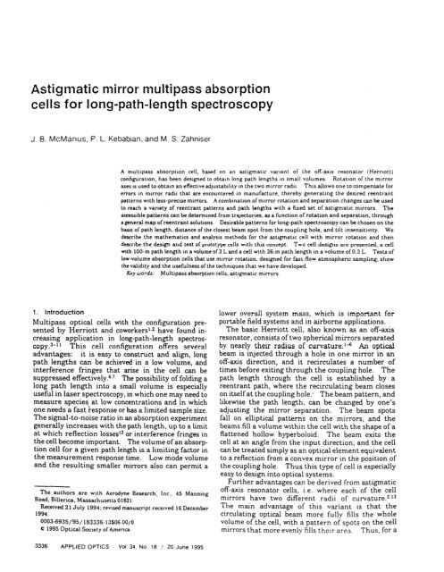
<strong>Astigmatic</strong> <strong>mirror</strong> <strong>multipass</strong> <strong>absorption</strong><br />
<strong>cells</strong> <strong>for</strong> <strong>long</strong>-<strong>path</strong>-<strong>length</strong> spectroscopy<br />
J. 6. McManus, P. L. Kebabian. and M. S. Zahniser<br />
A <strong>multipass</strong> absorptton cell, based on an astigmatx variant of the off-axis resonator (Herrtott)<br />
contiguratton. has been desrgned to obtain <strong>long</strong> <strong>path</strong> <strong>length</strong>s in small volumes. Rotatron of the mtrror<br />
axes 1s used to obtam an effective adjustabtlity in the two <strong>mirror</strong> radii. Thus allows one to compensate <strong>for</strong><br />
errors rn <strong>mirror</strong> radii that are encountered In manufacture, thereby generating the dewed reentrant<br />
patterns wth less-precise <strong>mirror</strong>s. A combination of <strong>mirror</strong> rotation and separation changes can be used<br />
to reach a variety of reentrant patterns and <strong>path</strong> <strong>length</strong>s with a fixed set of astigmatic mu-rors. The<br />
accessible patterns can be determined from trajectories, as a function of rotation and separation. through<br />
a general map of reentrant solutions. Desirable patterns <strong>for</strong> <strong>long</strong>-<strong>path</strong> spectroscopy can be chosen on the<br />
basis of <strong>path</strong> <strong>length</strong>. distance of the closest beam spot from the coupling hole, and tilt insensitivity. We<br />
describe the mathematics and analysis methods <strong>for</strong> the asttgmatic cell with mtrror rotation and then<br />
describe the design and test of prototype <strong>cells</strong> with this concept. Two cell designs are presented, a cell<br />
tith 100-m <strong>path</strong> <strong>length</strong> in a volume of 3 L and a cell with 36-m <strong>path</strong> <strong>length</strong> in a volume of 0.3 L. Tests of<br />
low-volume <strong>absorption</strong> <strong>cells</strong> that use <strong>mirror</strong> rotation. designed <strong>for</strong> fast-flow atmospheric sampling, show<br />
the validity and the usefulness of the techniques that we have developed.<br />
Key words: Multipass <strong>absorption</strong> <strong>cells</strong>, asttgmatic <strong>mirror</strong>s<br />
1. Introduction<br />
Multipass optical <strong>cells</strong> with the configuration presented<br />
by Herriott and coworkers1.2 have found increasing<br />
application in <strong>long</strong>-<strong>path</strong>-<strong>length</strong> spectroscopy.z-‘1<br />
This cell configuration offers several<br />
advantages: it is easy to construct and align, <strong>long</strong><br />
<strong>path</strong> <strong>length</strong>s can be achieved in a low volume, and<br />
interference fringes that arise in the cell can be<br />
suppressed effectively.6.7 The possibility of folding a<br />
<strong>long</strong> <strong>path</strong> <strong>length</strong> into a small volume is especially<br />
useful in laser spectroscopy, in which one may need to<br />
measure species at low concentrations and in which<br />
one needs a fast ‘response or has a limited sample size.<br />
The signal-to-noise ratio in an <strong>absorption</strong> experiment<br />
generally increases with the <strong>path</strong> <strong>length</strong>, up to a limit<br />
at which reflection losses*2 or interference fringes in<br />
the cell become important. The volume of an <strong>absorption</strong><br />
cell <strong>for</strong> a given <strong>path</strong> <strong>length</strong> is a limiting factor in<br />
the measurement response time. Low mode volume<br />
and the resulting smaller <strong>mirror</strong>s also can permit a<br />
The authors are with Aerodyne Research. Inc.. 45 Manning<br />
Road. Billerica. MassachusettsO1821.<br />
Received 21 July 1994; revised manuscript recerved 16 December<br />
1994.<br />
0003-6935/95/183336-13$06.00/O.<br />
0 1995 Optical Society of America<br />
lower overall system mass, which is important <strong>for</strong><br />
portable field systems and in airborne applications.<br />
The basic Kerriott cell, also known as an off-axis<br />
resonator, consists of two spherical <strong>mirror</strong>s separated<br />
by nearly their radius of curvature.rd An optical<br />
beam is injected through a hole in one <strong>mirror</strong> in an<br />
off-axis direction, and it recirculates a number of<br />
times be<strong>for</strong>e exiting through the coupling hole. The<br />
<strong>path</strong> <strong>length</strong> through the cell is established by a<br />
reentrant <strong>path</strong>, where the recirculating beam closes<br />
on itself at the coupling hole: The beam pattern, and<br />
likewise the <strong>path</strong> <strong>length</strong>, can be changed by one’s<br />
adjusting the <strong>mirror</strong> separation. The beam spots<br />
fall on elliptical patterns on the <strong>mirror</strong>s, and the<br />
beams fill a volume within the cell with the shape of a<br />
flattened hollow hyperboloid. The beam exits the<br />
cell at an angle from the input direction, and the cell<br />
can be treated simply as an optical element equivalent<br />
to a reflection from a convex <strong>mirror</strong> in the position of<br />
the coupling hole. Thus this type of cell is especially<br />
easy to design into optical systems.<br />
Further advantages can be derived from astigmatic<br />
off-axis resonator <strong>cells</strong>, i.e. where each of the cell<br />
<strong>mirror</strong>s have two different radii of curvature.2.‘3<br />
The main advantage of this variant is that the<br />
circulating optical beam more fully fills the whole<br />
volume of the cell, with a pattern of spots on the cell<br />
<strong>mirror</strong>s that more evenly fills their area. Thus, <strong>for</strong> a<br />
3336 APPLIED OPTICS Vol 34. No. 16 / 20 June 1995
given number of passes through the cell, the beam<br />
spots are more widely spaced than in other types of<br />
<strong>cells</strong> (conventional Herriott <strong>cells</strong> or White ceils”),<br />
permitting smaller mode volumes and smaller <strong>mirror</strong>s.<br />
One difficulty that has discouraged the USC of<br />
astigmatic <strong>cells</strong> has been the need <strong>for</strong> extreme preci-<br />
SIOII In the manufacture of the <strong>mirror</strong>s. One may<br />
need to define two different radii with an accuracy of<br />
1 part in 10’ to ensure that the pattern will close<br />
With a spherical <strong>mirror</strong> cell. changes tn the <strong>mirror</strong><br />
spacing can accommodate errors 111 the radll, and the<br />
desired pattern always can be achieved With astigmatlc<br />
<strong>mirror</strong>s, a reentrant condition must be establlshed<br />
<strong>for</strong> two axes simultaneously, so adlustment of<br />
the <strong>mirror</strong> spacing alone cannot compensate <strong>for</strong> both<br />
axes. Circumventing this problem by one’s stressing<br />
the <strong>mirror</strong> is possible, but this would be unwieldy<br />
In many applications. We have Investigated a<br />
method13 of adjusting <strong>for</strong> <strong>mirror</strong> radii errors by<br />
rotating one <strong>mirror</strong> about its optical axis. This<br />
allows us to compensate <strong>for</strong> manufacturing errors in<br />
the radii, permitting the nlirrors to be made with<br />
relaxed tolerances and reduced cost.<br />
An additional advantage of the use of ihe <strong>mirror</strong>twist<br />
degree of freedom is that other reentrant patterns,<br />
corresponding to different <strong>path</strong> <strong>length</strong>s, become<br />
accessible with a given set of <strong>mirror</strong>s. By<br />
translating and rotating the <strong>mirror</strong>s, one can use a<br />
variety of cell patterns and <strong>path</strong> <strong>length</strong>s. This can<br />
be especially useful during setup, when a shorter <strong>path</strong><br />
<strong>length</strong> may be desired. Small changes in <strong>mirror</strong><br />
separation and twist also may be used to establish<br />
<strong>path</strong> <strong>length</strong>s that are significantly greater than the<br />
nominal design.<br />
In this paper we describe the mathematics and<br />
analysis methods <strong>for</strong> the astigmatic cell with <strong>mirror</strong><br />
rotation and then describe the design and test of<br />
prototype <strong>cells</strong> with this concept. We review the<br />
basic reentrant equations <strong>for</strong> astigmatic <strong>cells</strong> and<br />
then discuss methods of selecting favorable reentrant<br />
patterns. We show how <strong>mirror</strong> rotation can be used<br />
to accommodate <strong>mirror</strong>-manufacturing errors and to<br />
achieve different patterns. We then show how the<br />
set of all possible patterns can be organized in a<br />
coordinate space-and how one can move through that<br />
space by changing <strong>mirror</strong> separation and rotation.<br />
Two prototype low-volume <strong>absorption</strong> <strong>cells</strong> that use<br />
<strong>mirror</strong> rotation have been designed <strong>for</strong> fast-flow<br />
atmospheric sampling. The larger cell has a 100-m<br />
<strong>path</strong> <strong>length</strong> in a volume of 3 L, and the smaller cell<br />
has a 36-m <strong>path</strong> <strong>length</strong> in a volume of 0.3 L. Tests of<br />
these <strong>cells</strong> show the validity and the usefulness of the<br />
techniques we have developed.<br />
2. Cell Analysis<br />
A Basic Reentrant Equations<br />
The circulation of the beams within the cell can be<br />
described approximately with the equations presented<br />
by Herriott and coworkers ’ L The location of<br />
the centroid of the beam on each <strong>mirror</strong> is described<br />
by sinusoidal equations, with an angular advance on<br />
each pass, 0, that is a function of the <strong>mirror</strong> radii and<br />
spacing. In this simplified analysis, the two <strong>mirror</strong>s<br />
are assumed to be identical. \vlth no tilt or rotation<br />
This analysis is an idealization of the beam propagation<br />
that IS useful <strong>for</strong> an understanding of the basic<br />
bchavlors of the cell. especially the rcenlrant beam<br />
patterns A description with 1 x 4 matrIces, presentcd<br />
below. IS used to account <strong>for</strong> the effects of<br />
rotation of the <strong>mirror</strong> principal axes with respect to<br />
each other, as well as <strong>mirror</strong> tilt and nontdentical<br />
<strong>mirror</strong>s.<br />
With astigrnatlc <strong>mirror</strong>s,? there are two lndepcndent<br />
reentrant equations that describe the ctrculatlon<br />
of beams wlthln the cavltv. _ A single integer 1 IS used<br />
to count the beam reflections from both <strong>mirror</strong>s, as IC<br />
the spot patterns were combined on a single plane<br />
The s-v coordinates of the lth beam spot are gven b!<br />
x, = X0 sinllex), y, = Y, sm(10,),<br />
D<br />
0, = cos-’ ( 1 - p 1 t e,=cos-ll--, (1,<br />
I ( R, 1<br />
where X0 and Y0 define the size of the overall spot<br />
pattern, R, and R, are the <strong>mirror</strong> radii of curvature (if<br />
we assume that the two <strong>mirror</strong>s are identical), and D<br />
is the <strong>mirror</strong> separation. Thus the beam spots trace<br />
out a <strong>path</strong> on the <strong>mirror</strong>s that is sinusoidal in x and y<br />
but with different frequencies (i.e., a Lissajous pattern).<br />
For <strong>cells</strong> close to confocal spacing (D = RI,<br />
one has 0, = 7712 and 8, = ::;‘2. The reentrant<br />
condition is that the beam exits after N passes, I.e..<br />
xN=yh’= 0, which is satisfied <strong>for</strong><br />
NO, = M=T, N9,, = M+ (2)<br />
which yields the following <strong>for</strong> reentrant patterns:<br />
8, = nM,/N, 8) = srM,/N. (3)<br />
The integers N, M,, and -M, define the pattern of<br />
transits through the cell. A choice of (N, M,, M,j<br />
and a base <strong>length</strong> <strong>for</strong> the cell will result in design<br />
values <strong>for</strong> the <strong>mirror</strong> radii. In this basic description<br />
of the reentrant conditions, with the entrance and<br />
exit at the center of one <strong>mirror</strong>, N must be even (an<br />
integral number of round trips). For these patterns<br />
to be unique in terms of (N, M,, M,( there must be no<br />
common factors (other than 21 within this set of<br />
integers. If there are such factors, the pattern is<br />
degenerate, and at this value of 8, and 8, a pattern<br />
with a lower pass number (reduced by the common<br />
factor) will be supported by the cell.<br />
The size of a spot pattern on the <strong>mirror</strong>s is set by<br />
the imtlal alming of the first beam Into the cell at<br />
coordinates X0 and & That lnltlal spot will be near<br />
the maxImum radius of the overall spot pattern. and<br />
the rest of the beam-spot tocz:!nns will result from
the initial aiming; The pattern must be large enough<br />
that the recirculating beams avoid exiting through<br />
the coupling hole be<strong>for</strong>e intended. If the closest<br />
spots to the coupling hole are relatively far away in a<br />
given pattern, the whole pattern size may be reduced.<br />
We find it convenient to define reduced angularadvance<br />
variables +, and 4, where<br />
4, = 0, - 5 ’ e$y = 0, - 5. (4)<br />
For nearly confocal <strong>cells</strong>, 4, = 0 and bY = 0. We<br />
have used the + variable in our earlier discussion of<br />
cell algebra,6 and the results here are similar. In<br />
terms of the <strong>mirror</strong> radii and spacing we have<br />
+Iy = sin or, <strong>for</strong> D = R,<br />
4 ry = g-1.<br />
i SY 1<br />
Thus the 4 variables are approximately the distance<br />
in separation from confocal spacing <strong>for</strong> the separate<br />
radii, normalized by those radii. The arguments of<br />
the b’s are the negatives of the usual resonator<br />
parameters,15 g,, = (1 - D/R,,). 4 ranges from<br />
-u/Z (at D = 0 or R,, = =) to +u/2 at (D/R,, = 2).<br />
For DIR,, > 2, hy is undefined, but this corresponds<br />
to unstable resonator’conditions (g2 > l), so<br />
this range is unimportant practically. The 4’s also<br />
may be defined <strong>for</strong> reentrant patterns as<br />
(5)<br />
4ry = (6)<br />
Because we usually deal with patterns in nearly<br />
confocal <strong>cells</strong>, we have N = 2M, A new pair of<br />
pattern variables, k,, KY, may be defined as<br />
k, =N-2Mx, k,=N-2My (7)<br />
The k’s are even integers, which are small compared<br />
with MxJ, that are related to various pattern characteristics.<br />
In this case the reentrant 4 variables<br />
become :<br />
4ry = -bG)k,y/N. (8)<br />
There are numerous patterns of recirculating<br />
beams, as defined by choices of (N, M,, My) and different<br />
choices in this set can have beam-spot patterns<br />
with very different appearances. All the patterns<br />
are within a rectanguk.r boundary, but there will be<br />
different distances <strong>for</strong> the closest approach of spots to<br />
the coupling hole and diRerent sensitivities to misalignments<br />
of the <strong>mirror</strong>s. Examples of a few of<br />
these patterns (<strong>for</strong> the front <strong>mirror</strong>) are shown in<br />
Figs. l-3. Figure 1 shows a symmetrical pattern<br />
with even M, and MY and spots far from the coupling<br />
o” 0<br />
0 0<br />
00<br />
00<br />
0 0<br />
0 0 0<br />
0 O 0 0<br />
0 0<br />
0 0 -<br />
@<br />
0 O 0<br />
0 0<br />
0<br />
0<br />
0 0 0<br />
0 O 0 0<br />
0 00<br />
0 0”<br />
0<br />
00 0 0 00<br />
0<br />
00<br />
OO 0<br />
0 00 O0 0 0 O 0 OO<br />
Fig. 1. Symmetrical pattern (N = 182. M, = 80, M,, = 76). with<br />
even M,, and with spots far from the coupling hole. Only spots on<br />
the input <strong>mirror</strong> are shown. For all figures, a circle indicates the<br />
coupling hole.<br />
hole. Figure 2 shows a pattern with spots close to<br />
the hole. Figure 3 shows an asymmetrical pattern,<br />
with odd My.<br />
The coordinates of the beam spots fall on the<br />
Lissajous curve given by Eq. (l), where the ratio of<br />
frequencies is 0,/C+ = MJM,. The beam spots lie<br />
widely separated on this curve, so the spot pattern<br />
often looks unlike a familiar continuous Lissajous<br />
figure. In some cases the beam spots appear to lie on<br />
other Lissajous curves that are much coarser than<br />
those defined by the ratio MJM,. One can understand<br />
this effect by expressing the spot coordinates<br />
with reduced angles. If one considers only the front<strong>mirror</strong><br />
beam spots, their coordinates can be reduced<br />
when multiples of IT are removed from the sine<br />
moo0 0 0 0 0 0 0 0 ooow<br />
Qx)-z.00 0 0 0 0 0 0 cl OOOOD<br />
030000000@000000Qp<br />
Qcx)oooo 0 0 0 0 0 0000~<br />
moo0 0 0 0 0 0 0 0 000003<br />
Fig. 2. Pattern (190, 80. 761, with even M,, but with spots close<br />
to the hole Only spots on the input <strong>mirror</strong> are shown.<br />
3338 APPLIED OPTICS / Vol. 34. No. 18 / 20 June 1995
go0 ‘oooo 0 08<br />
O Oo 0 0 o" O<br />
O 0 0 O<br />
8" 0 0 "B<br />
0<br />
0<br />
0<br />
/a O<br />
0<br />
0 0<br />
0 0<br />
0 0<br />
0 0<br />
0<br />
0<br />
0<br />
0 : o” Oo o<br />
8 0 0 0<br />
00 O<br />
0<br />
0<br />
o 0”<br />
0 0 00 0 00 0 o”<br />
O<br />
0<br />
0<br />
0<br />
8<br />
OO 8<br />
Fig 3. AsymmetrIcal pattern 188. 86. 83:. with odd .4f, Only<br />
spots on the input <strong>mirror</strong> are show-n<br />
argument<br />
in Eqs. (1) yielding<br />
x, = (- 1)’ sin (j:h,/N), y, = ( - l)-‘ sin (j&,/N),<br />
where j counts the returns to the front <strong>mirror</strong>, i.e.,<br />
j = i/2. These coordinates lie on a Lissajous curve<br />
defined by the frequency ratio k,/k,. Similar arguments<br />
can be used to generate back-<strong>mirror</strong> reduced<br />
coordinates. In some cases even coarser curves can<br />
be generated by subtraction of multiples of 217 from<br />
the arguments in Eqs. (9). The value of the necessary<br />
multiple, which is different <strong>for</strong> x and y, can be<br />
found from Diophantine equations.i6 Similarly, the<br />
reduced frequency ratio fv/fx is found from integer<br />
solutions to be k,f, - k,f, = 2N.<br />
One usually cannot tell by simple observation of<br />
the spot pattern what the pattern parameters are.<br />
When one sets up a practical cell, changing the <strong>mirror</strong><br />
spacing causes a variety of nearly reentrant spot<br />
patterns to appear without an obvious sequential<br />
order. Identification generally requires that observed<br />
patterns be matched with calculated ones and<br />
that one possesses a detailed knowledge of the relation<br />
of patterns to each other.<br />
B. Properties of Spot Patterns and Advantageous Choices<br />
Advantageous patterns may be chosen <strong>for</strong> <strong>absorption</strong><br />
experiments in which the <strong>path</strong> <strong>length</strong> is <strong>long</strong> (large<br />
N), the beam pattern is compact, and the fringe levels<br />
are small Generally we use <strong>cells</strong> that are close to<br />
confocal, because this results in the minimum mode<br />
sizes <strong>for</strong> the propagating beam, yielding a smaller cell.<br />
Interference fringes produced in the cell can be made<br />
to appear at higher frequency (<strong>for</strong> greater ease of<br />
suppression) when the spots neighboring the coupling<br />
hole are nearly midway through the beam’s<br />
orbit.6 Patterns that are less sensitive to <strong>mirror</strong> tilt<br />
may also be chosen, so that intermediate beam spots<br />
(9)<br />
will be less susceptible to being driven out the coupling<br />
hole by misalignments.<br />
Patterns with even M, and I?, correspond to whole<br />
numbers of complete transverse oscillations of the<br />
beams in the cell by the use of Eqs. (2). The output<br />
beam <strong>for</strong> these patterns will exit from the diagonal<br />
corner in the square pattern; i.e., the last spot in the<br />
cell is at (x:y) = (- 1. - 1) <strong>for</strong> the first spot at (1, 1).<br />
In this case the beam will act as if it is reflecting from<br />
a <strong>mirror</strong> (equivalent to the back of the cell-input<br />
<strong>mirror</strong>) in the position of the input plane of the cell.<br />
This is a great advantage in the application of these<br />
<strong>cells</strong> to laser systems. and we use these patterns<br />
exclusively. These patterns also are more symmetrical<br />
in the distribution of spots on the <strong>mirror</strong>s than<br />
patterns with either :%I, or M, odd. The even M,,<br />
patterns are insensItIve to trlt. as can be seen by the<br />
total cell transfer matrix being unity [as explained<br />
below). With M, and M, even. N/2 must be odd to<br />
avoid common factors.<br />
For application to low-volume <strong>cells</strong>, we select patterns<br />
with the innermost spots on the input <strong>mirror</strong><br />
far from the center. Naturally, this permits the use<br />
of smaller <strong>mirror</strong>s and smaller mode volumes.<br />
There is a relatively large set of patterns with a<br />
similar wide spacing from the center available, and<br />
<strong>for</strong> -these patterns the spacing scales as<br />
l/I jc No 18 ;\P=‘LIE3 OPTICS 3339
&. M&ix Analysis of Mirror Rotation and lilt -<br />
A 4 x 4 matrix description of the cell allows us to<br />
investigate the effects of rotation of the <strong>mirror</strong>s about<br />
the optical axis, nonidentical <strong>mirror</strong>s, and <strong>mirror</strong> tilt.<br />
Once we derive a matrix description of a single<br />
traverse of the cell, the location and slope of a ray<br />
after N traverses results from the cell matrix raised to<br />
the Nth power, multiplying the input ray vector.<br />
Because we allow several nonideal effects to occur, the<br />
matrix descriptions tend to produce complex analytical<br />
expressions. There<strong>for</strong>e many of the results of<br />
the matrix analysis are achieved numerically.<br />
The geometry of the cell configuration is shown in<br />
Fig. 4. Concave astigmatic <strong>mirror</strong>s are located at z =<br />
0 and z = D. The principal radii of curvature, R, and<br />
Rb, are nominally aligned with the x and the y<br />
coordinate axes, respectively. A beam is injected<br />
into this system at x = y = z = 0, and it propagates<br />
between the two <strong>mirror</strong>s. We are concerned primarily<br />
with the transverse (x-y) position of the beam on<br />
each return to the <strong>mirror</strong> at z = 0. The basic<br />
geometry may be modified by rotation of the axes of<br />
the two <strong>mirror</strong>s with respect to each other by an angle<br />
0!. This rotation provides the added degree of freedom<br />
needed to correct <strong>for</strong> errors in the cell ‘radii,<br />
when it is used together with an adjustment of cell<br />
<strong>length</strong>.<br />
A propagating ray is represented by a column<br />
vector 2, with components [x, x’, y, y’], where x’ and<br />
y’ are the slopes in thex andy directions, respectively.<br />
The ray matrix <strong>for</strong> one cycle of the beam’s propagation<br />
through the cell is constructed from free-space<br />
propagation D(D) and <strong>mirror</strong> reflection matrices<br />
WC, Rd:<br />
t-2 = R(% Rb)D(D)R(&,, &)D(D). (10)<br />
The coordinate of the beam spot after n cycles, Z,, is<br />
given by CT&, where Z, is the initial vector with x =<br />
Y = 0. For <strong>mirror</strong> spacing (D) and <strong>mirror</strong> principle<br />
radii (R,, Rb) aligned with the coordinate axes, the<br />
I \<br />
Fig. 4. Ckom t e r-y of the cell with <strong>mirror</strong> axis rotation<br />
component matrices are given by<br />
D(D) =<br />
[l<br />
0<br />
D<br />
100<br />
0 01<br />
I<br />
OOlD'<br />
I<br />
0 0 0 1<br />
1 1 0 0 Ol<br />
I<br />
R(RcmRb) = o o 1 o . (11)<br />
-2/R., 0 01 -2/f& 0 o 1 i<br />
When the <strong>mirror</strong> principal axes are aligned with the<br />
coordinate axes, the cell matrix is block diagonal, with<br />
uncoupled 2 x 2 matrices <strong>for</strong> x and y motion. When<br />
the <strong>mirror</strong> axes are rotated by an angle 0, to the<br />
coordinate axes, the reflection matrix becomes<br />
R’UL Rd = T(-WW,, R,)T(e,), (12)<br />
where T(0,) is the rotation matrix,<br />
i cos 0 8, cos 0 8, sin 0 Bc sin 0 0. 1<br />
‘WV = -sin e o . cos e -’ . (13)<br />
I I I 0<br />
I<br />
1 0 -sin Br 0 cos 8, J<br />
The rotation matrices mix x and y components of the<br />
beam coordinates. Nevertheless the behavior of the<br />
cell is substantially similar to the unrotated case,<br />
with essentially sinusoidal x and y spot motions.<br />
The frequencies are altered and the overall pattern<br />
becomes mildly distorted, but complete reentrant<br />
patterns still can be achieved.<br />
We have explored the behavior of the <strong>multipass</strong> cell<br />
matrix by direct computation using a program written<br />
in the MATLAB langt~age.~~ We directed our initial<br />
ef<strong>for</strong>ts at finding the spacing and twist adjustments<br />
necessary to make up <strong>for</strong> errors in the <strong>mirror</strong> radii.<br />
For this type of calculation, we start with a set of<br />
<strong>mirror</strong> radii and a spacing that corresponds to a given<br />
reentrant, pattern. Then the <strong>mirror</strong> radii are assumed<br />
to deviate from those values by a small<br />
amount. We change the spacing by an amount S and<br />
change the <strong>mirror</strong> twist 0, so that the beam again<br />
exits the cell in the same pattern. For small deviation<br />
in the radii, the solution (8,, 6) that causes the<br />
beam to exit results in a slightly distorted version of<br />
the nominal pattern. When 0, and D are found by<br />
adjusting them to make the last spot in the pattern<br />
return to the origin, the resulting cell matrix CNi2 is<br />
the identity matrix (<strong>for</strong> even M, and M ), to within<br />
numerical tolerances. As an example of this adjustment<br />
procedure <strong>for</strong> the pattern (N = 182, M, = 80,<br />
My = 76) (Fig. l), we assume <strong>mirror</strong> errors of 2 X<br />
10A3, i.e., R, = RJ1.002 and Rb = RJ0.998. The<br />
required adjustments are 8, = -17.02” and 6/D =<br />
-3.93 x 10⁻⁴.<br />
3340 APPLIED OPTICS / Vol. 34. NO. 18 / 20 June 1995
We have used the matrix description of the cell to<br />
search systematically <strong>for</strong> advantageous patterns <strong>for</strong><br />
spectroscopic applications. The primary search has<br />
been in terms of finding patterns with wide spacing<br />
around the coupling hole. The search has been<br />
restricted to even M,, My, and odd N/2. Figure 1<br />
shows an example of one such pattern with good<br />
spacing. Other properties can be included in the<br />
search, as outlined above. The effect of our tilting<br />
the <strong>mirror</strong>s with respect to the cell z axis also has<br />
been investigated. Tilt can be accounted <strong>for</strong> by the<br />
addition of a constant to the slopes, (x’ ory’), at each<br />
reflection. As expected, in patterns with even M,<br />
and MI the coordinates of the last spot are insensitive<br />
to tilt.<br />
In addition to compensating <strong>for</strong> manufacturing<br />
errors, <strong>mirror</strong> rotation and separation changes can be<br />
used to achieve a variety of reentrant patterns that<br />
would not be possible with an unrotated set of<br />
astigmatic <strong>mirror</strong>s. This gives a valuable degree of<br />
flexibility to the astigmatic cell design. With <strong>mirror</strong><br />
rotation, we can select from a set of different <strong>path</strong><br />
<strong>length</strong>s with a single set of <strong>mirror</strong>s, similar to the<br />
selection of different reentrant patterns in the nonastigmatic<br />
cell through separation changes alone.<br />
.<br />
D. Iterative Equations and Recirculation Frequencies in<br />
the <strong>Astigmatic</strong> Cell<br />
Although the above 4 x 4 matrix description gives us<br />
the <strong>mirror</strong> spacing and rotation <strong>for</strong> pattern closure<br />
through numerical simulation, it would be desirable<br />
to have corresponding analytical expressions. The<br />
4 x 4 matrix description may be reduced to a pair of<br />
coupled difference equations18 that naturally yield<br />
analytical expressions <strong>for</strong> circulation frequencies in<br />
the cell. This approach, which we outline below, is<br />
analogous to the 2 x 2 matrix description of nonastigmatic<br />
(i.e., spherical) <strong>mirror</strong> off-axis resonators and<br />
the reduction of such a matrix to a single difference<br />
equation. I9 With the 4 x 4 matrix expressions <strong>for</strong><br />
one and two complete mund trips of the cell, the<br />
coordinates of the beam spot on the nth return to the<br />
front <strong>mirror</strong> (x,, y,,) are found in terms of the previous<br />
coordinates:<br />
where<br />
X” = (A* - 2 - e*)x,-, - x,,w2 + Ey,Ml,<br />
yn = (B* - 2 - e*)y,-, - yn..* - E xndl, (14)<br />
A = 2 - [(a,D)cos* T + (d)sin* T],<br />
B = 2 - [(a$)sin* T + (a&)cos* T]<br />
e = (1/2)(a, - q)D sin(27),<br />
E = -(l/4)1(%<br />
- ab)D]*sin(4r),<br />
and where a, = 2/R,, q = 2/R&, T = 6,/2; i.e., T is one<br />
half the total rotation angle between the <strong>mirror</strong>s.<br />
In the basis used here, the <strong>mirror</strong>s are rotated<br />
symmetrically by +T and -1. The coupling term E.<br />
usually will be small. If the coupling were zero in<br />
Eqs. (14), the resultant motions would be*&usoidal<br />
inx andy, with cosines of the angular advances in two .<br />
passes given by (A’ - 2 - e’)/2 and (B’ - 2 - e*)/2.<br />
The coupled difference equations can be expresssed<br />
in the <strong>for</strong>m of a 2 x 2 matrix with the A? operator,<br />
Azx, = x,,, - %I,, + x, m2:<br />
(151<br />
with /, = (A’ - 2 - eZ) and /,. = (B’ - 2 - e’). This<br />
pair of equations is analogous to the pair of differential<br />
equations <strong>for</strong> coupled oscillators. The motions<br />
of coupled oscillators are described by shifted normal<br />
mode frequencies that are arrived by one’s diagonalizing<br />
the matrix <strong>for</strong> the coupled equations. In a<br />
similar fashion, the difference equation matrix can be<br />
diagonalized to yield shifted normal mode frequencies<br />
<strong>for</strong> circulation through the cell. The results are, <strong>for</strong><br />
the cosines of the angular advances in two passes,<br />
cos or* = ( 1/2)(Az - 2 - e* - Q.<br />
cos ey2 = (1/2)(B* - 2 - e* + 0, (16)<br />
with 5 = (1/2)(B* - A*)(- 1 + [ 1 - 4Ez j(B* - A2)*]11 *.<br />
When 5 -=x(B* - A*), 5 = -&*/(B2 - A’).<br />
These angular advances describe the motion of<br />
compound variables that are linear combinations of x<br />
and y, although the amount of mixing is small.<br />
However, <strong>for</strong> reentrant patterns both x and y will<br />
simultaneously be zero when the beam exits, so the<br />
mixed variables will be zero as well. There<strong>for</strong>e the<br />
angles given in Eqs. (16) can be used to find reentrant<br />
solutions in the astigmatic <strong>cells</strong> with rotated <strong>mirror</strong><br />
axes.<br />
E. Beam Escape and Maps of Pattern Location<br />
When the <strong>mirror</strong> spacing is displaced from the exact<br />
reentrant condition, the last beam spot is swept<br />
across the coupling hole. The tolerance <strong>for</strong> spacing<br />
changes, i.e., the range over which the beam still falls<br />
within the coupling-hole diameter (dh), is a function<br />
of the pass number and the various cell parameters.<br />
To express the spacing tolerance, we define a transverse<br />
spot velocity IJ, = dS/dD, where S is the lateral<br />
position of the last beam spot on the input <strong>mirror</strong>.<br />
The tolerance then is AD = dh/u,. Based on Eq. (l),<br />
the (vector) spot velocity is<br />
u, = 3?X,i cos(iO,)[D(2R, - D)]-’ *<br />
+ yY,i cos(iCl,)[D(2R, - D)]-“*. (17)<br />
For the last spot, i = N and cos(NB) = ~1.<br />
Furthermore, if& = Y0 = ( 1/J2)Ro, and D = RzJ, the<br />
scalar velocity is approximately<br />
“* = (1/J2)NRo([D(2R, - D))-’ f [D(2R, - D)]-‘I’/*<br />
= NR,/D. (18)<br />
Thus, as the number of passes increases, the spot<br />
20 June 1995 VOI 34, No If3 APPLIED OPTICS 334 1
velocity increases proportionately, and the <strong>mirror</strong>spacing<br />
tolerance becomes correspondingly tighter.<br />
If the <strong>mirror</strong> spacing changes beyond the tolerance<br />
range, the beam pattern will change, yielding a<br />
greater or a smaller number of passes be<strong>for</strong>e the<br />
beam exists. This behavior may be investigated<br />
numerically if we assume a set of <strong>mirror</strong> radii, derive<br />
cb, and 6, as a function of <strong>mirror</strong> spacing from<br />
relations (5), and iterate the beam coordinates until<br />
the spot falls within the coupling-hole radius, i.e., it<br />
escapes. A plot of the number of passes as a function<br />
of <strong>mirror</strong> spacing <strong>for</strong> a fixed set of <strong>mirror</strong> radii has an<br />
irregular appearance. Indeed, in tests of actual <strong>cells</strong>.<br />
changing the <strong>mirror</strong> separation permits the beam to<br />
exit in many nearly reentrant patterns with a widely<br />
varying number of passes, without apparent logical<br />
progression.<br />
A general map of the location of reentrant solutions<br />
In the two-dimensional space of (4,. 6,) can provide a<br />
more complete picture of astigmatic cell behavior.<br />
At an arbitrary point (c$,, &, I. one may calculate how<br />
many times the beam circulates be<strong>for</strong>e it escapes.<br />
The recirculating beam escapes at cycle j, (N = 2,)<br />
when the beam coordinate is within the coupling-hole<br />
radius p (ignoring the finite beam size), I.e.,<br />
sin*(2j,&,) + sin’(2j,,&,) < 13~.<br />
Here the hole radius is normalized by the overall<br />
pattern size, or X,, = Y. = 1. The result of iteration<br />
of relation (19) is shown in Fig. 5, in which the escape<br />
pass number is plotted <strong>for</strong> the region -0.2 < 6, <<br />
-0.18, -0.27 < &I~ < -0.25. Forachoiceof<strong>mirror</strong><br />
radii and spacing within an appropriate range, one<br />
can WxIate 4, and $ and find the corresponding<br />
number of passes from Fig. 5. The “+-space” plot,<br />
N(p, &:, 6,). is a general map of the location of<br />
reentrant patterns that is independent of specific<br />
choices of cell parameters. The plot is made up of<br />
overlapping circular zones (or radius P;N), each<br />
supporting a single spot pattern with a constant pass<br />
number corresponding to nearly reentrant conditions.<br />
For a zone with pass number N and zone center<br />
coordinates (da,. $,.), the pattern parameters can be<br />
recovered from Eqs. (8). When larger zones completely<br />
or partially overlie smaller ones. the beam<br />
esits in the lower pass-number pattern.<br />
The b-space plot can be constructed by the use of<br />
geometric methods to produce maps of nearly reen-<br />
Leant solutions with higher accuracy and more quickly<br />
than b!. numerical iteration of relation i 19). The<br />
constructlon algorithm. described In Appendix A. also<br />
elucidates the structure of the solution space. Such<br />
3 constructed plot is shown in Fig. 6. The plot of<br />
~L:IP< 6,. &I shown in Figs. 5 and 6 Includes beam<br />
escapes In any direction from the cell. If we consider<br />
only patterns In which the beam exits in the opposite<br />
quadrant from the input [i.e., the ( - 1, - 1) quadrant],<br />
then a more sparse &space plot results, as shown in<br />
Fig. 7. These zones correspond to even M, and hi!,<br />
and odd N/2, i.e., where the cell behaves like a<br />
<strong>mirror</strong>, which is the subset that we use in practical<br />
cell designs.<br />
For a fixed set of <strong>mirror</strong> radii, changing the <strong>mirror</strong><br />
spacing generates a nearly linear trajectory through<br />
this (6,. do,) space. Relations 5 may be considered a<br />
-.ZSO<br />
Phiy<br />
-.270<br />
-.200 ..;os -.ioo -.16S -.160<br />
Phh<br />
Fig. 5. Iterated solution <strong>for</strong> cell escape as a functron of 6.. br, with<br />
normalized hole radius p = 0.1. The logarithm of the number of<br />
passes is encoded as tone. The location of pattern ir\I = 182.<br />
M, = 80. M, = 76) is indicated<br />
Fig. 6 Plot of *ones of nearly reentrant patterns constructed<br />
wl:h the algorithm described in Appendix A. Patterns with the<br />
beam exlrlng m any dlrection up to a limiting number of 1000<br />
round trips are shown The location of our pattern wth 182<br />
passes IC indicated<br />
3342 APPLIED OPTICS Vol 34 No 18 20 June 1095
Phiy<br />
0.260<br />
:;i; w !irV LOCP-<br />
-l<br />
1.6 1.65 2.3 2.66 a<br />
0-J<br />
- There are several approximations that -al’e built<br />
into the use of these maps to find cell patterns. The<br />
maps are idealized and general. without effects that<br />
are specific to particular <strong>mirror</strong>s or implementations.<br />
The maps do not include <strong>mirror</strong> tilt, which would<br />
tend to smear odd-M zones. The maps do not include<br />
the effects of pattern distortion that occur at<br />
larger <strong>mirror</strong>-rotation angles, which would also lead<br />
to distortion of the zones. The maps also do not<br />
include the effect of re-aiming the input beam.<br />
Despite these approximations, the maps are a useful<br />
tool in cell setup.<br />
3. Prototype Cell Designs and Test Results<br />
4.270<br />
Fig. 7. Plot of zones of nearly reentrant patterns constructed<br />
with the algorithm described In Appendix A. Patterns with the<br />
beam exiting in the f - 1. -l! quadrant only; up to a limiting<br />
number of 1000 passes, are shown. Trajectories showing the<br />
patterns accessible to the system as the <strong>mirror</strong> separation and<br />
rotation angle are changed are drawn. The three lines are <strong>for</strong><br />
spacing changes (tics are placed at intervals of 0.2% of the base<br />
<strong>length</strong>) with fixed <strong>mirror</strong> axis angles of O’, 22’. and 30’.<br />
parametric equation <strong>for</strong> 6, and $J in terms of D.<br />
The trajectory may be expressed directly as<br />
4190<br />
Phlx<br />
$.,(b,) = sin-‘(7 sin 6, + (Y - l)], (20)<br />
where y = R,/Rb. If b is small, then &CC&) =<br />
[Ydh + (Y - 111.<br />
The above analysis provides an expression [Eqs.<br />
(16)] <strong>for</strong> the cosines of the angular-advance angles as<br />
a function of <strong>mirror</strong> rotation and spacing. From<br />
Eqs. (16), one can derive a trajectory through the<br />
(&J,, 4) plane as the <strong>mirror</strong> rotation and spacing are<br />
adjusted. Such a set of trajectories is shown in Fig. 6<br />
<strong>for</strong> a set of <strong>mirror</strong>s that is designed to access the<br />
pattern { 182;‘80, 76) at a rotation angle of 22”. As in<br />
Eq. (20), these trajectories are nearly linear when the<br />
rotation angle is fixed.<br />
Together the maps and trajectories in 4 space<br />
provide useful tools in setting up astigmatic <strong>cells</strong>.<br />
One can locate desirable and accessible patterns and<br />
move to them with the right combination of translation<br />
and rotation of the <strong>mirror</strong>s. At the initial setup<br />
of a cell, errors in the <strong>mirror</strong> radii can be seen as an<br />
offset in the location of the patterns from their<br />
expected values. Using the map, one can then determine<br />
the actual <strong>mirror</strong> radii. If one wants to move<br />
between patterns with different total <strong>length</strong>s, the<br />
map and trajectory plot shows what combination of<br />
translation and rotation is needed.<br />
A. Cell Designs. 100 and 36 m<br />
We have produced astigmatic <strong>cells</strong> with the <strong>mirror</strong>twist<br />
concept <strong>for</strong> application to fast-response atmospheric<br />
trace-gas sampling.‘0-22 The low mode volume<br />
af<strong>for</strong>ded by the astigmatic design is critical in<br />
such applications. Two cell designs have been constructed:<br />
the larger one has a <strong>path</strong> <strong>length</strong> of 100 m<br />
in a base <strong>length</strong> of 0.55 m and a volume of 3.2 L, and<br />
the smaller one has a <strong>path</strong> <strong>length</strong> of 36 m in a base<br />
<strong>length</strong> of 0.2 m and a volume of 0.3 L. Both of the<br />
<strong>cells</strong> are based on a nominal 182 passes in the pattern<br />
(N, M,, My] = { 182, 80, 761. As described in Section<br />
2, it is possible to align these <strong>cells</strong> to have pass<br />
numbers between approximately 0.5 and 2 times the<br />
nominal number of passes. Both of these <strong>cells</strong> have<br />
been used in laboratory and field measurements.<br />
The 100-m cell has been used in measurements of<br />
HO2 line broadening*O and in combustion diagnostics.*’<br />
The 36-m cell has been incorporated in a<br />
tunable diode laser based system <strong>for</strong> fast (lo-20-Hz)<br />
concentration measurements <strong>for</strong> eddy correlation<br />
determinations of trace-gas fluxes to the atmosphere.**<br />
We primarily describe the larger fast-flow cell,<br />
because we have done the most extensive tests on it<br />
and the smaller cell is very similar. The design of<br />
the larger cell is shown in Fig. 8. The cell structure<br />
is built on an aluminum base with a glass tube center<br />
section. End assemblies hold the <strong>mirror</strong>s, provide<br />
optical access, shape the-gas flow, and pressure-seal<br />
the cell.’ The front <strong>mirror</strong> is bolted directly to the<br />
front flange with no adjustments. The rear <strong>mirror</strong> is<br />
mounted with a post-and-collar arrangement to permit<br />
<strong>length</strong> and rotation adjustments. An alignment<br />
jig is attached to the <strong>mirror</strong> support post during setup<br />
and alignment. After setup, the <strong>mirror</strong> post is locked<br />
to the collar, the alignment jig is removed, and the cell<br />
cover plate is attached.<br />
The <strong>mirror</strong>s are made of aluminum in the <strong>for</strong>m of<br />
octagons that are 7.6 cm across. The active cell<br />
volume, defined by the cylindrical space between the<br />
<strong>mirror</strong>s, is 8.6 cm in diameter and 55 cm <strong>long</strong>,<br />
yielding a total volume of 3.2 L. The volume occupied<br />
by the beams is defined to the first order by the<br />
square spot pattern on the <strong>mirror</strong>s ( - 5 cm on a side).<br />
yielding - 1.4 L. The <strong>mirror</strong> size in this design is<br />
20 June 1995 ‘.‘Ol 34 r40 18 APPLIED OPTICS 3343
Exhaust ’ \ 0. Ring<br />
Pap*<br />
EX?UUSl<br />
Plwlurn ‘*<br />
Mlnw<br />
SSll<br />
1Ocm<br />
t<br />
FIN. 8. Cross-secttonal view of the 100.m-<strong>path</strong>.len@h. 3.2-L fast-flow cell. The cell IS shown lo scale. with an overall <strong>length</strong> of 66.7 cm<br />
and a diameter of 15 cm.<br />
based on considerations of mode size at the maximum<br />
design wave<strong>length</strong> of 10 pm. We have used the<br />
criterion that the separation between the input beam<br />
and the closest recirculated beam spot on the input<br />
<strong>mirror</strong> should be 10 times the Gaussian beam radius<br />
(intensity). The coupling-hole radius (0.44 cm) is<br />
then one half the distance to the nearest beam spot.<br />
This yields a conservative design that may be made<br />
tighter in applications in which cell volume is at a<br />
premium.-<br />
The scaling of the cell volume with pass number,<br />
base <strong>length</strong>, and wave<strong>length</strong> can be estimated simply<br />
if we consider the case of nearly confocal <strong>cells</strong>. A<br />
recirculating beam matched to a confocal cell has all<br />
the beam spots the same size, w,, at ,z times the<br />
radius at the center of the cell, wg = (Ad:‘2~;)’ *, where<br />
d is the <strong>mirror</strong> spacing. For a pattern width of W,<br />
the maximum s acing between spots, S, is approximately<br />
S = W/ P N. If we equate the pattern spacing<br />
with some factor a times the spot radius w,, we arrive<br />
at the design pattern width, W = a(kdN.‘T;)’ *, and<br />
the volume V = dW* = a*hd*Ni-rr. Thus the volume<br />
will scale as the square and the <strong>mirror</strong> width will scale<br />
as the square root of the base <strong>length</strong>. The scaling<br />
arguments will change somewhat <strong>for</strong> departures from<br />
the confocal condition or if beams that are injected<br />
are not matched to the cell. However, the above<br />
argument shows the general trend of scaling. With<br />
our small-cell base <strong>length</strong> (20 cm), which is 0.36 times<br />
that of the larger cell, we designed the <strong>mirror</strong> width to<br />
be somewhat smaller (a factor of 0.5 rather than 0.6)<br />
than would result from the scaling argument. The<br />
factor of 2.8 reduction in <strong>path</strong> <strong>length</strong> yielded a<br />
factor-of-10 decrease in volume.<br />
An inlet system was designed to supply a uni<strong>for</strong>m,<br />
low-pressure flow.of the sampled gas to the optical<br />
measurement volume. Rapid response of the cell<br />
depends on one’s maintaining as uni<strong>for</strong>m a flow as<br />
possible with a minimum of recirculation zones that,<br />
by trapping gas and slowly releasing it to the main<br />
flow, would degrade the response. We typically operate<br />
the cell at a pressure of -30 Torr. This pressure,<br />
at which the collisional and the Doppler widths<br />
are approximately equal, is optimum <strong>for</strong> atmospheric<br />
trace-gas analysis. We maintain the pressure in the<br />
fast-flow cell pumping at a fixed volume flow (10 L. s),<br />
with a sonic inlet nozzle at the end of a 1.73~cm-i.d.<br />
sampling tube. The sonic inlet nozzle is a stainlesssteel<br />
conical tip with an inlet orifice 0.16 cm in<br />
diameter. The nozzle is tapered on the inlet side and<br />
polished throughout the conical expansion to the<br />
sampling tube to ensure smooth flow into the sampling<br />
probe tube. The cell inlet is shaped to direct<br />
the flow past the <strong>mirror</strong> and into the volume smoothly.<br />
At 30 Torr, the flow is laminar, with a Reynold’s<br />
number of - 400. The mean flow velocity in the<br />
cylindrical optical volume is (10 L/s)/‘((n/4) (8.5<br />
cm)*] = 176 cm/s. The mean residence time is the<br />
<strong>length</strong> of the optical cell divided by the mean flow<br />
velocity, (55 cm)/(176 cm/s) = 0.31 s. The gas exits<br />
around the periphery of the input <strong>mirror</strong> and enters<br />
an exhaust plenum, which helps to maintain uni<strong>for</strong>m<br />
circumferential flow around the downstream <strong>mirror</strong>.<br />
B. Cell Tests<br />
The cell-per<strong>for</strong>mance issues include ease of setup to<br />
the desired pattern, optical loss, optical fringe levels,<br />
and flow response. The flow response includes a<br />
comparison between the expected and the actual<br />
flowing-gas replacement times. The cell has been<br />
tested with infrared light derived from a tunable<br />
diode laser operating near 2200 cm-i (4.5 Frn) and<br />
140Ocm-i (7.5 prn).*O The tunable diode laser spectrometer<br />
allows <strong>for</strong> frequency-stabilized and rapidly<br />
swept laser operation with rapid (up to 30 Hz) data<br />
collection and display. The data acquisition is based<br />
on rapid-sweep integration over the full infrared<br />
transition line shape with synchronous measurement<br />
of the transmitted infrared light intensity. Two<br />
molecules were observed in the lests, nitrous oxide<br />
(N20) and water vapor, as examples of nonsticky and<br />
sticky molecules, respectively. The N20 line monitored<br />
was at 2197.699 cm-’ and had a line strength of<br />
5.4 x lo-i9 cm2 molecules-’ cm-i. The water transition<br />
was at 1329.9 cm-i and had a line strength of<br />
4 x lo-** cm2 molecules-’ cm-’ at 296 K.<br />
3344 APPLIED OPTICS I( Vol. 34. No 18 20 June 1995
C. Optical Setup<br />
A carefully coaligned visible trace laser beam makes<br />
infrared beam alignment relatively simple, and setup<br />
of the desired reentrant pattern can be accomplished<br />
rapidly. We have typically aligned the cell to operate<br />
on the 182-pass pattern but also have tested it at 90,<br />
274. 366, and 454 passes by making small changes in<br />
the <strong>mirror</strong> separation and twist. The maps of the<br />
pass number as a function of spacing and twist (Fig.<br />
7) make the setup operation much easier. Typically<br />
one will not know the precise spacing of the <strong>mirror</strong>s,<br />
and small manufacturing errors lead to further uncertainty<br />
as to the initial C$ coordinates. Being able to<br />
move among a set of reentrant solutions adds confidence<br />
that the location in C$ space is known and that<br />
the identificatidn of higher-order patterns is correct.<br />
The final step in the setup is to confirm that the cell<br />
spot pattern corresponds to the calculated patterns.<br />
Generally we achieve a very close match between<br />
observed and calculated patterns. An example is<br />
shown in Fig. 9 <strong>for</strong> the 182-pass pattern with a 17”<br />
<strong>mirror</strong> rotation.<br />
The infrared beam in the tunable diode laser<br />
spectrometer is at a high f-number (> 40), with a<br />
focus near the center of the cell. This yields a beam<br />
that is nearly matched to the cell, where.the -recirculating<br />
beam maintains a nearly constant size at the<br />
<strong>mirror</strong>s. This yields the minimum cell-volume con-<br />
dition. If the focus is made closer to the coupling<br />
hole, the beam spots on the outer edges of the <strong>mirror</strong>s<br />
become larger. However, changing the input-focusing<br />
condition within reasonable limits does not<br />
strongly affect the transmission through the cell.<br />
The cell transmission as a function of pass number<br />
was measured to check reflection losses. The transmission<br />
at 2200 cm-l <strong>for</strong> the 182-pass pattern is 20%,<br />
yielding a <strong>mirror</strong> reflectivity of 99.2%. which is<br />
consistent with specifications <strong>for</strong> the enhanced silver<br />
coating. We have also tested the fringe levels <strong>for</strong> the<br />
Cell near 2200 cm-‘. The high-frequency. (0.005-<br />
cm-‘) fringe amplitude on the transmitted beam is<br />
-5 x 10-S p.-p. This detected fringe amplitude is<br />
probably lower than the actual amplitude because<br />
there is a frequency jitter on the laser of - 1 x 10-J<br />
cm-‘, which will wash out the highest-frequency<br />
fringes ( > 10-m source <strong>length</strong>).<br />
0. Flow-Response Tests<br />
We per<strong>for</strong>med flow-response tests by rapidly injecting<br />
small amounts N20 or H20 into a stream of carrier<br />
gas (dry nitrogen) Rowing through the cell and then<br />
by measuring the spectral contrast of <strong>absorption</strong> lines<br />
as a function of time. The gas was injected both as<br />
an impulse and as a rectangular wave. The first<br />
experiment measured the time response of the fast-<br />
Row cell to an impulse of N20. supplied by a pulsed<br />
valve (Veeco Model pv-10) with a response time of a<br />
few milliseconds. The output of the valve mixed<br />
rapidly with a carrier gas and entered the flow-cell<br />
sampling orifice in less than 10 ms. The result of the<br />
pulse-response experiment is displayed in Fig. 10.<br />
The rise time of the <strong>absorption</strong> signal is 40 ms and is<br />
limited by the response time of the data-acquisition<br />
system. This is not surprising because the gas transit<br />
time from the orifice to the optical volume is less<br />
than 5 ms. Hence the total time delay between the<br />
pulsed valve and the optical volume is no more than<br />
15 ms, and the time blurring is presumably even less.<br />
The <strong>absorption</strong> signal decays with a much <strong>long</strong>er time<br />
constant (T - 300 ms), which can be fitted to a single<br />
exponential decay over 2 orders of magnitude. The<br />
time constant <strong>for</strong> this decay is equal to the expected<br />
pump-out time <strong>for</strong> the 3-L cell with a lo-L/s pumping<br />
speed. As Fig. 10 shows, at least 99% of the gas flow<br />
can be accounted <strong>for</strong> by single exponential decay.<br />
No <strong>long</strong> time tailing is apparent, which suggests that<br />
the flow cell is well mixed on a 100-ms time scale.<br />
A second N20 experiment with rectangular-wave<br />
Fig. 9. Comparison of calculated and observed rear-<strong>mirror</strong> spot patterns <strong>for</strong> the patkrn (182, 80, 76). The caJcula& pattern IS on the<br />
left and includes 17’ of rotation between the <strong>mirror</strong> axes. The spot diameter decreases exponentially 10 slmo!ate decreasing brightness,<br />
.A photograph of the observed spot pattern. with a visible trace beam. is shown on the right<br />
20 June 1995 : Voi 34, tic ‘: A-Z=_ ~2 ,Z?TICS 3345
i<br />
“1,~: )<br />
tim~” (second:;<br />
20<br />
Fig. 10. Response of the IOO-m-<strong>path</strong>-<strong>length</strong>. 3.2-L fast-flow cell to<br />
an impulse of NsO. With a pumping speed of 5 L/s. the Rushing<br />
time 010.33 s (a 3-s-r rate)<br />
gas injection provides further evidence that the cell<br />
flow is well mixed on short time scales. The result of<br />
this experiment is displayed in Fig. 11. The optical<br />
response signal is roughly a rectangular wave, but<br />
both the rising and the falling edges are rounded.<br />
As is shown in Fig. 11, the rising edge is I well<br />
described by an exponential approach to the peak<br />
signal, and the falling edge is well described by an<br />
exponential decay. The time constants in each case<br />
are approximately equal to the 300-ms pump-out<br />
time <strong>for</strong> the cell. This is exactly the result expected<br />
when the impulse response function of Fig. 9 is<br />
convolved with a sharp rectangular wave. A careful<br />
look at Fig. 11 reveals a small deviation between the<br />
observed signal and the fit to it in the tail of the signal<br />
decay. It is not clear whether this weak, <strong>long</strong> time<br />
tail is a property of the cell or an irregularity of the<br />
pulsed valve. Its appearance seemed to be intermittent<br />
and is of little practical consequence.<br />
Our final flow-response test with the larger cell was<br />
with a sticky molecule, water. In principle, the<br />
response of the cell to a sticky molecule such as water<br />
vapor might be much more sluggish than <strong>for</strong> a<br />
nonsticky molecule (N,O), because of surface adsorp-<br />
Fig. 12. Response of the 100.m-<strong>path</strong>-<strong>length</strong>. 3.2-L fast-flow cell to<br />
a rectangular wave of HsO. The recorded stream data are shown<br />
by the dotted curve. and an exponential fit to the fall is shown as a<br />
solid curve. With a pumping speed of 5 L/s, the flushing time is<br />
0.33 s (a 3-s-r rate).<br />
tion-desorption. In this experiment we tested the<br />
step response by rapidly switching between ambient<br />
(humid) air and dry nitrogen. The result, displayed<br />
in Fig. 12, shows very little <strong>long</strong> time tailing from<br />
surface effects. There may be a trace of a <strong>long</strong> time<br />
component, but its amplitude is no more than 1% of<br />
the total signal.<br />
A similar set of tests was conducted <strong>for</strong> our smaller<br />
cell design. This 36-m-<strong>path</strong>-<strong>length</strong> cell, with a volume<br />
of 0.27 L, was tested at a pumping speed of 5<br />
L/s. In Fig. 13 we show the result of injecting a<br />
square wave of CH,. The response time of 0.04 s is<br />
consistent with the cell volume and pumping speed.<br />
These response-time tests have shown that the<br />
response of the cell is strongly dominated by a single<br />
exponential component whose characteristic time is<br />
determined by the cell volume divided by the pumping<br />
speed. This suggests that the cell is well mixed<br />
on a fast scale and that further improvements in<br />
response time may be achieved with smaller <strong>cells</strong> and<br />
bigger pumps. This is an important consideration in<br />
atmospheric-sampling appiications that require subsecond<br />
response times, such as eddy correlation flux<br />
measurements.22 Furthermore, the water responsetime<br />
tests indicate that surface effects <strong>for</strong> sticky<br />
molecules may be overcome by high-volume laminar<br />
I<br />
. :: : I---\<br />
f L ‘\ \ i yorallme<br />
CL<br />
i?i 0.17 b&o me late =3.5 s"<br />
3<br />
c :<br />
i<br />
= l<br />
L<br />
g 1.<br />
L<br />
0.01<br />
j<br />
I<br />
I<br />
-3.4 s-’<br />
\<br />
,h<br />
$%Yl<br />
: ,L<br />
0 S 10 1S<br />
time (seconds)<br />
Fig. 11. Response of the lOO-m-<strong>path</strong>-<strong>length</strong>, 3.2-L fast-flow cell to<br />
a rectangular wave of NsO. The recorded data stream is shown by<br />
the dotted curve. and exponential tits to the rise and fall are shown<br />
as solid curves. With a pumping speed of 5 L/s, the Rushing time<br />
is -0.29 s (a 3.4-3.5-s-t rate).<br />
0 5 10 15 20 2s 30<br />
TIME<br />
(sea.ods)<br />
Fig. 13. Response of the 36-m-<strong>path</strong>-<strong>length</strong>, 0.27-L fast-flow cell to<br />
a square wave of CH, With a pumping speed of 5 L/S. the<br />
flushing time is 0 04 s la 25-s-i rate)<br />
3346 APPLIED OPTICS / Vol 34. No. 18 / 20 June 1995
flow. This is important in sampling a variety of<br />
atmospheric species that either interact with surfaces<br />
(e.g., NHS, HN03) or that are reactive (e.g., H02).*0<br />
4. Conclusions<br />
In conclusion, we have explored the application of<br />
astigmatic <strong>mirror</strong>s to <strong>multipass</strong> <strong>absorption</strong> <strong>cells</strong> <strong>for</strong><br />
fast-flow spectroscopic applications. By rotating the<br />
<strong>mirror</strong>s about their optic axis, we can make up <strong>for</strong><br />
finite manufacturing tolerances and can make a<br />
variety of reentrant patterns accessible. Thus the<br />
same set of <strong>mirror</strong>s can be used to provide a range of<br />
<strong>path</strong> <strong>length</strong>s by making small changes in the <strong>mirror</strong><br />
separation and rotation angle. We have developed<br />
techniques <strong>for</strong> mapping the available patterns and<br />
have shown how the patterns are reached with <strong>mirror</strong><br />
separation and rotation.<br />
We have designed and tested <strong>absorption</strong> <strong>cells</strong> with<br />
the <strong>mirror</strong>-rotation concept. The technique IS useful<br />
and easy to apply. The cell designs have base<br />
<strong>path</strong> <strong>length</strong>s of 100 m (in 3.6 L) and 36 m (in 0.27 L),<br />
w:th 182 passes in their nominal reentrant patterns.<br />
Other patterns have been accessible with <strong>mirror</strong><br />
rotation and separation changes, which permits <strong>path</strong><br />
<strong>length</strong>s between 0.5 and 3 times the nominal values.<br />
The <strong>cells</strong> show flow-response times consistent with<br />
their active-volumes and show low fringe levels.<br />
Appendix A. Structure of “0 Space”<br />
In this appendix we describe in more detail the<br />
properties of the solution space <strong>for</strong> relation (19),<br />
which gives us the number of passes be<strong>for</strong>e escape <strong>for</strong><br />
arbitrary 4 coordinates, N(p, +,, +,.). As noted above,<br />
a plot of N(p, +,, $-“) shows overlapping circular zones<br />
(of radius p/N), each supporting a single spot pattern<br />
with a constant pass number corresponding to nearly<br />
reentrant conditions. The radius of the zones can be<br />
understood when the velocity of the last spot is<br />
expressed in terms of the do coordinates. Considering<br />
first +,, we obtain dX,/d$, = N cos N+, = N,<br />
with similar results <strong>for</strong> 6,. The tolerance in 4 is<br />
then A+ = p/N, where p-is the <strong>mirror</strong>-hole radius<br />
normalized by the pattern size.<br />
Plots of N(p, b,, by), as shown in Figs. 5 and 6, show<br />
striking patterns of high complexity with structure<br />
on a wide range of scales. N(p, +,, 9) is highly<br />
symmetrical, with all the quadrants of ++,, *&<br />
having the same structure, with the additional symmetry<br />
of reflection about the 45” line within the<br />
quadrants. If one starts at a point N(p, b,, +Y), with<br />
a corresponding (N, K,, k,) spot pattern and moves to<br />
a corresponding point N(p, &,‘, b,‘), the cell spot<br />
patterns are related in specific ways. For coordinate<br />
exchange, (b,‘, 4,‘) = (by, b,), the patterns of spots on<br />
the <strong>mirror</strong>s are rotated by 90” but are otherwise<br />
identical. For sign changes, (+,‘, $‘) = (-&,, -+,),<br />
the new patterns are (N, (N - M,), (N - MY)), which<br />
are very similar to the initial patterns. If one starts<br />
from a given pattern, one will be able to use <strong>mirror</strong><br />
scparatlon and rotation changes to reach the vicinit)<br />
of only one other equivalent pattern. the one with a<br />
sign change in both 4 coordinates.<br />
One way to understand the structure 0fN(p, 6,“, 6,)<br />
is through a consideration of the exact reentrant<br />
solutions to relation (19) which occur at<br />
Nb, = I,n, Iv+, = I,:. (Al I<br />
<strong>for</strong> some Integers I, and f, BCcauSC thC solutions<br />
are slmultancous. we have<br />
4,./d), = I, 1, (A2 1<br />
Thus, <strong>for</strong> any point (&,, +,), the number of passes can<br />
be found from Eq. (Al) and from the lowest integer<br />
ratlo <strong>for</strong>med from the coordmates. provided that the<br />
point IS not overlaid by another zone with lower N<br />
One can construct a map of h’ip. d)., b,,) efficiently b><br />
organlzlng the reentrant solutions into lines through<br />
the 16,. 6,) plane with slopes of Integer ratios. 11, =<br />
il, I,)b, = ~f:,/k,&. Here we Identify the Integers<br />
I, and I, with k, and k, in Eqs. (81 The set of line<br />
slopes is <strong>for</strong>med by the set of k,.‘k,, where there are<br />
no common factors (other than 2). For a given range<br />
of id,, 4,) on a line, the values of 6, or by that yield an<br />
even, integral N [from Eqs. (811 yields a set of<br />
first-order solutions on the line. These solutions<br />
produce zones of radius p/N at the (6,. by) coordinates.<br />
All the spot patterns found on a gven k,/k, line fall<br />
on the same reduced Lissajous curve. The number<br />
of slope ratios needed is limited by the requirement<br />
that the lowest-order solutions on the line, within a<br />
given Q range, are less than some maximum N, which<br />
is set by cell loss. Thus one need not consider the<br />
infinite set of rational slopes in filling the (b,, 6,)<br />
plane, but only up to a limiting size of numerator and<br />
denominator.<br />
One complication in this filling method <strong>for</strong> the<br />
(+,, bYI) plane with nearly reentrant zones is that<br />
there are higher-order patterns on each line of KY/k,.<br />
The higher-order patterns are where k, and k, are<br />
both multiplied by some integer and the resulting N’s<br />
are nearly, but not exactly, multiplied by the same<br />
integer. The higher-order patterns are interleaved<br />
symmetrically between each pair of first-order patterns.<br />
For an interval on-a line between first-order<br />
patterns, N, and N,+i, the interleaved patterns have<br />
N = f,(N) + 2f), w h ere Z[ is the interleave factor and -<br />
f is a rational fraction in the range O-l <strong>for</strong>med as<br />
f = j/If, with no common factors between integers j<br />
and Ifi<br />
The above procedure can be used to reproduce the<br />
N(p, b,, 4,) zone map analytically, more rapidly and<br />
with higher accuracy than the point-by-point stepping<br />
through 4 space that was used to generate Fig. 5.<br />
It is essentially a systematic way to fill the plane with<br />
zones located at points where the coordinates are in<br />
integer ratios to each other, up to some limiting size<br />
of the integers used. The procedure is amenable to<br />
an ordered construction from high to low denominators<br />
so that zones of lower N generally overlie zones of<br />
higher N. An additional sorting step may be needed<br />
20 June 1995 : Vol 34. No 1.3 A?PLlED OPTICS 3347
to ensure that all the lower N zones overlie the higher<br />
N zones. A synthetic N(p, &, $.) map is shown in<br />
Fig. 6, which corresponds to the same region as Fig. 5.<br />
The construction algorithm also shows the nature of<br />
the solution space, which is controlled by the set of<br />
irreducible rational fractions, the Farey sequence.23.2’<br />
The Farey sequence describes both the set of lines of<br />
solutions in + space and the interleaving of higherorder<br />
solutions on the lines.<br />
We are grateful to the National Science Foundation<br />
<strong>for</strong> partial support of this work through grant ISI-<br />
890768 1.<br />
References<br />
I D. R. Herrloil. H. Kogelmk. and R Kompfner, “Off-axls <strong>path</strong>s<br />
In spherlcal <strong>mirror</strong> resonators.” Appl. Opt. 3,523-526 I 1964 I<br />
2 0. R Herrlott and H J Schuke. “Folded optical delay hnes.”<br />
Appl Opt 4.883-889 I 19651.<br />
3 W R Trutna and R L Byer. “MultIpIe-pass Raman gain cell.‘.<br />
Appl Opt 19. 301-312 I 19801.<br />
4 J AJiltmann. R. Baumgart. and D. C. Weltkamp, “Two-<strong>mirror</strong><br />
multIpass <strong>absorption</strong> cell,” Appl. Opt. 20.995-999 (1981).<br />
5 D. Kaur. A. M. de Souza. J. Wanna. S. A. Hammad,<br />
L. Mercorelli. and D. S. Perry, “Multipass cell <strong>for</strong> molecular<br />
beam <strong>absorption</strong> spectroscopy.” Appl. Opt. 29.119-124 (19901<br />
6 J. B. McManus and P. L. Kebabian. “Narrow optical interfer.<br />
ence fringes <strong>for</strong> certain set-up conditions in <strong>multipass</strong> <strong>absorption</strong><br />
<strong>cells</strong> of the Herriott type.” Appl. Opt. 29.898-900 (1990r.<br />
7 J. A. Silver and A. C. Stanton. “Optical interference fringe<br />
reduction in laser <strong>absorption</strong> experiments,” Appl. Opt. 27,<br />
1914-1916(1988).<br />
8. J. B. McManus, P. L. Kebabian. and C. E. Kolb. “Atmospheric<br />
methane measurement instrument using a Zeeman.spllt<br />
He-Ne laser.” Appl. Opt. 28,5016-5023 (1989).<br />
9. J. B. M~MXILIS. P. L. Kebabian. and C. E. Kolb. “The Aerodyne<br />
Research Mobile Methane Monitor.” in Measurement ofAlmospheric<br />
Gases. H. I. Schiff. ed., Proc. Sot. Photo-Opt. Instrum.<br />
Eng. 1433.330-339 I 1991).<br />
10. S. M. Anderson and M. S. Zahniser. “Open-<strong>path</strong> tunable diode<br />
laser <strong>absorption</strong> <strong>for</strong> eddy correlation flux measuremen& of<br />
atmospheric trace gas=” in Measurement of Almosphertc<br />
Gaws, in H. 1. SchifT. cd.. Prop. Sot. Photo-Opt. instrum. Eng.<br />
1433.167-178llSSll.<br />
11. C. R. Webster. R. D. May, C. A. Trimble. R. c. Chave, and<br />
J. Kendal, “Aircraft (ER-21 laser infrared <strong>absorption</strong> spectrometer<br />
(ALIASI <strong>for</strong> in-&u stratospheric measurements of HCl,<br />
N1O. CH,. NOI. and HNO>.” Appl. Opt. 33.454-472 (1994).<br />
12. P. Wcrle and F Slemr. “Signal-to-noise ratio analysis in laser<br />
<strong>absorption</strong> spectromelcrs using optical mullipass <strong>cells</strong>.” Appl.<br />
OPL. 30.430-434 ( 19911.<br />
13 I’ L. Kcbablan. “OIT-axis cnv~ty absorpLlon cdl.” U.S. patent<br />
5.291.265(1 March 19941.<br />
I4 J U White. “Long opttcal <strong>path</strong>s of large aperlurc,” J. Opt<br />
.%c. Am 32. ‘285-288 (1942)<br />
I5 H Kogelmk and T LI. “Laser beams and resonators.” Proc<br />
IEEE% 1312-1329(196Gl.<br />
IG M R Schroeder. Ntrrnber Theo? IR Sctencc and Communtca-<br />
([on. Vol 7olSpnngerSer1es1n In<strong>for</strong>mationSciences(Springer-<br />
Verlag. Be&n. 19861<br />
17 sl.1TL48 (Mach \Vorks. Inc Natlck. Mass.. 19901<br />
IS R E hllcken;. Dlflccrcrtce Eq[rorrorts (Van Nostrand ReInhold.<br />
New York. 196;l<br />
19 A Yanv. QU(III(URI Elecrronlcs. 2nd ed (Wdey. New York.<br />
19751. p I03<br />
20. D. D. Nelson and M S. Zahniser. “Air-broadened linewidth<br />
measuremenls in the vz vibrattonal band of the hydroperoxyl<br />
radical,” J. Mol. Spectrosc. 166.273-279 (1994).<br />
21. J Wormhoudt. M S Zahniser. D. D. Nelson, J. B. McManus.<br />
R C. Miake-Lye. and C. E. Kolb. “Infrared tunable diode laser<br />
diagnostics <strong>for</strong> aircraft exhaust characterization,” in Laser<br />
Applications tn Combustton and Combustion Diagnosks II.<br />
R. J. Locke. ed. Proc. Sot Photo-Opt. Instrum. Eng. 2122.<br />
49-60 (; 19941<br />
22 C. E. Kolb, J. C. Wormhoudt. and M. S. Zahnizer, “Recent<br />
advances in spectroscopic instrumentation <strong>for</strong> measuring stable<br />
gases in the natural environment,” in Mefhods in Ecology:<br />
Trace &es. P. A. Matson and R. C. Harriss, eds. (Blackwell.<br />
Boston). to be published.<br />
23 D. L. Gonzalez and 0. Piro, “Symmetric kicked self oscillators:<br />
Iterated maps, strange attractors and symmetry of the phaselocking<br />
Farey sequence,” Phys. Rev. L&t. 55, 17-19 (1985).<br />
24. T. Allen. “On the arithmetic of phase locking: coupled neurons<br />
as a lattice on II*.” Physica 6.305-320 (1983).<br />
2348 APFLltC Cl)i’TICS VCI 34 No i8 30 June IS95