Long solitary internal waves in stable stratifications

More documents

Recommendations

Info

176 W. B. Zimmerman and J. M. Rees: Long solitary waves Table 2. Characterization of the solitary solutions (34) to the hybrid BBM-KdV Eq. (35), where λ 4 = 0, and ZR (22) equations for Ri = 10 and various k, ε pairs. k ε C BBM-KdV 2 BBM-KdV C ZR 2 ZR 0.05 -1 0.570442 0.725191 0.5336 0.972316 0.05 -6 3.42446 0.120865 2.72698 0.312483 0.05 -12 6.84866 0.0604326 4.82226 0.215112 C = −3k2 (1 + ελ 4 ) + ελ 3 (4 + 3ελ 4 ) ( D k 2 ) + 2ελ 3 )) ( k + (λ 2 (3k 2 2 ) + 2ελ 3 + ελ 3 + λ 1 D λ 1 D √ × −6ε 2 λ 1 λ 2 λ 3 λ 4 + ( ( λ 2 3k 2 ) + ελ 3 − 3λ1 (1 + ελ 4 ) ) 2 2 = −2λ ( 2 3k 2 ) + ελ 3 + 3 (1 + ελ 4) + 2 ελ 1 λ 3 ελ 3 ελ 1 λ √ 3 × −6ε 2 λ 1 λ 2 λ 3 λ 4 + ( ( λ 2 3k 2 ) + ελ 3 − 3λ1 (1 + ελ 4 ) ) 2 where ( ) D = −λ 2 3k 2 + 11ελ 3 + 3λ 1 (1 + ελ 4 ) (46) √ + −6ε 2 λ 1 λ 2 λ 3 λ 4 + ( ( λ 2 3k 2 ) + ελ 3 − 3λ1 (1 + ελ 4 ) ) 2 For Ri = 10 and small k and ε, the asymptotic expansion of Eq. (46) yields ( C = 0.1035 k 2 + −0.5705 − 0.09778 k 2) ε + O (k 4 , ε 2 ) ( 2 = 0.2734 + k 2 −0.1061 + 0.1269 ) − 0.7257 + O (k 4 , ε)(47) ε ε This is closely comparable with the approximation of λ 4 = 0 of the last subsection. As it has just been shown that there is a new, analytic solution of the solitary wave form to a newly derived inviscid NEE, it is conventional to explore by numerical simulations along the lines of the seminal paper by Zabusky and Kruskal (1965) whether the solutions are soliton-like in character. Table 2 demonstrates the distinctly different solitary wave features for the two different solitary wave equations explored here – the ZR solitary wave is always broader and slower propagating due to the presence of the hypernonlinearity with coefficient λ 4 . 4.3 Numerical simulations of the nonlinear evolution equation (Christov and Velarde, 1995), as standard finite difference approximations were found to be inherently unstable. One technique that has demonstrated robust stability properties is the method of lines (MOL). Schiesser (2001) describes the salient features that the spatial discretization is established permanently in the simulation, but the temporal solution is adaptive, using local error estimates to adapt the time step to within the desired error tolerance. We coded the method of lines, using Runge-Kutta-Fehlberg (a 4–5 method) in time, and up to seven point differences to accomodate the A ξξξ term. Figure 8 shows the evolution of a single localized disturbance under the approximate KdV dynamics and of the ad hoc removal of the “BBM term” A ξξt , which has only the extra nonlinearity in addition to the KdV terms. Although this method proved adequate for the approximations attempted in Fig. 8, demonstrating the known analytic form of solution Eq. (34), it was not possible to include either the BBM term nor to resolve overtaking collisions of two initial disturbances. With the method of lines technique, the BBM term, A ξξt , can only be included consistently by finite difference approximations at the last time step. This delay contributes to numerical instability, which manifests as the inability to adapt the time step to the error tolerance. The collision simulation with MOL performs adequately with the KdV equation, with nonlinearity treated by delayed differences. However, the additional nonlinear terms form a shock wave upon collision which cannot be resolved by the technique. Since the difficulty lies within the delayed difference treatment of some terms, the prescribed solution is to use semiimplicit integration schemes. The workhorse method is the Crank-Nicholson scheme, which uses spatial centered differences arithmetically averaged between the current time and the future time step. These must be simultaneously solved. In the method adopted here, the linear terms are treated in the Crank-Nicholson fashion. The nonlinear terms are approximated by delays. The BBM term is treated by an Euler step in time, centered difference at both the current and future time. If A(ξ = jh, τ = nt) = A n j , where h is the spatial resolution, then a banded matrix equation results: It is well known that NEEs that are modified KdV equations are difficult to simulate numerically. For instance the KdV- KSV equation with both instability and hyperdiffusion terms required treatment by the method of variational embedding a 1 A n+1 j+2 + a 2A n+1 j+1 + a 3A n+1 j + a 4 A n+1 j−1 + a 5A n+1 j−2 = b 1 A n j+2 + b 2A n j+1 + b 3A n j + b 4A n j−1 + b 5A n j−2 +N ( ) A, A ξ , A ξξ , A ξξξ (48)
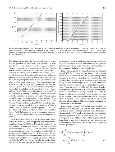
W. B. Zimmerman and J. M. Rees: Long solitary waves 177 time 250 200 150 100 50 0 -50 0 10 20 30 40 50 60 70 80 position x time (arbitrary scale) 45 40 35 30 25 20 15 10 5 0 0 10 20 30 40 50 60 70 80 position x Fig. 8. (a) Simulation of only the KdV terms in Eq. (35) and (b) Simulation of the all terms in Eq. (35) except the BBM A ξξt term; for Ri = 10 and k = 0.05, with an initial conditions of Eq. (34) with (a) ε = −6; (b) ε = −1 with origin shifted to x 0 = 10. Time is scaled arbitrarily so as to graphically separate successive time steps. In (a) t ∈ [0, 20]. In (b), t ∈ [0, 40]. Both simulations have spatial resolution h = 0.1 horizontally. The scheme is first order in time, second order in space. For the purposes of discussion, it is necessary to note only that a 1 = 1/2h 3 and a 3 = λ 1 /t − λ 2 /th 2 . Crank- Nicholson methods are absolutely stable (see e.g. Ganzha and Vorozhtsov (1996) for the von Neumann criterion). However, the sparse solver method becomes poorly conditioned if the matrix is not diagonally dominant, leading to spurious oscillations. Typically, for third order pdes, the condition for diagonal parity is that t ≈ h 3 , i.e. the first term of a 3 is of the same order as a 1 . This necessitates ridiculously small times steps t for any common choice of resolution in ξ, say 10 −2 . In this case, however, diagonal parity is achieved by balancing the second term of a 3 with a 1 , yielding t ≈ h. This is apparently a desirable situation from the standpoint of stability. Curiously, however, the system is poorly conditioned at achieving accuracy with decreasing t and h. As the second term in a 3 , which originates from the BBM term, always dominates the first term as h ↓, it is found that the linear terms in Eq. (48) approximate an identity operator on any signal A(ξ) at a given time. (b 3 has a similar structure, which leads to the mapping A n+1 j ← A n j as h ↓. Thus, only since λ 1 is naturally larger in modulus than λ 2 (see Table 1) is there a window in simulation parameter space (h, t) which is reasonably accurate and numerically stable. As an aside, it is possible to evade the whole issue of simulating the BBM A ξξτ term via applying the perturbation assumption. Peregrine (1966), in deriving the equation for an undular bore, noted that up to the order of the error in the perturbation scheme, A xxt ∼ A xxx . In this case, the fundamental assumption of a harmonic wave to leading order Eq. (18), allows the approximation λ 2 A ξξτ ∼ −k 2 λ 2 A τ , which is a minor modification to the accumulation term. However, this is formally only valid for ε ≪ 1. Indeed, although the NEE derived here Eq. (35), is formally only valid for small ε, in the case of high Ri (see Table 1), the coefficients of the nonlinear terms are naturally small, implying that large amplitude is possible before the practical requirement that the neglected terms are appreciable comes into force. Consequently, a robust simulation for large ε has practical value. Figure 9 demonstrates the Crank-Nicholson simulation of the full NEE Eq. (35) for single and double localized disturbance initial conditions of the form Eq. (34) appropriate to the analytic solution for C and . In contrast to the MOL solutions, here the solitary wave amplitude is taken as intrinsically positive, even though ε = −1. So these frames both represent waves of temperature and streamfunction depression. Frame (a) agrees roughly with the expected analytically predicted phase velocity C for the given conditions. Frame (b) demonstrates a clear phase shift – a boost to the larger, overtaking wave and a delay to the slower wave – due to the collision. The waves themselves appear unchanged at this resolution. These features establish the soliton-like character of the solutions (34) as originally established by Zabusky and Kruskal (1965). Contemporary connotations of soliton character imply that the equation is integrable (e.g. Cervero and Zurron, 1996), and thus an inverse scattering transform exists (for instance, Gardner et al., 1967) which permits the characterization of the time asymptotic state. Whether or not the NEE (35) is integrable is not addressed here. There is greater likelihood that it is integrable if it conserves wave energy, which is tested below. Multiplying the NEE by A, and integrating over all space yields: d λ 1 dt ∫ ∞ −∞ A 2 dξ = −λ 2 I 2 − k 2 ∫∞ −∞ AA ξξξ dξ ∫∞ + ελ 3 A 2 A ξ dξ − ελ 4 I 4 (49) −∞
Page 1 and 2: Nonlinear Processes in Geophysics (
Page 3 and 4: W. B. Zimmerman and J. M. Rees: Lon
Page 11: W. B. Zimmerman and J. M. Rees: Lon

Long solitary internal waves in stable stratifications

You also want an ePaper? Increase the reach of your titles

Delete template?

Save as template?