Long solitary internal waves in stable stratifications

More documents

Recommendations

Info

170 W. B. Zimmerman and J. M. Rees: Long solitary waves The separation constant was chosen to clarify that A must be a harmonic wave to leading order. If Eq. (18) holds, then the system (17) reduces to θ = φ y − ν [ φy (y − ν) − φ ] y − φ k2 (y − ν) φ + Ri y − ν = 0 (19) The second equation above is the well known Taylor- Goldstein equation (Taylor, 1931; Goldstein, 1931) for the particular case of a constant buoyancy frequency. For prescribed Ri, Eq. (19) is a two point boundary value problem (φ| y = 0 = φ| y = 1 = 0) for the eigenvalue ν. In the long wave limit, the regular spectrum (Davey and Reid, 1977) of ν n , n = ± 1, ±2, . . . , and the singular spectrum (Maslowe and Redekopp, 1980) (ν n ∈ [0, 1]) are known when Ri > 1/4. For 0 < Ri < 1/4, ν n are complex conjugates, implying that one harmonic wave grows without bound and the other decays. Zimmerman and Velarde (1997) demonstrate an analytic solution for the higher order dispersive terms in the long wave expansion and solvability condition, which is equivalent to the series solution to Eq. (19) in powers of k 2 : ν = c + ∞∑ k 2l s l (20) l=1 The first five s l were given in closed form for the regular modes. It was shown that the radius of convergence of the series s l is at least k r = 1 for all Ri and k r ≈ 10 for Ri ≫ 1. In general, with the exception of Ri ↓ 1/4, c ≫ s 1 ≫ s 2 ≫ etc., showing that phase velocity is highly insensitive to finite wavenumber effects. separation of the full system (14) only up to errors of O (ε). A ξξξ = −k 2 A ξ + O (ε) (21) The Ansatz that the full system separates with errors of O ( ε 2) is made with the error in Eq. (21) taking the explicit form A ξξξ = −k 2 A ξ − ε ∑ i λ i D (i) (ξ) (22) The unknown functions D (i) and coefficients λ i are determined by requiring that the O (ε) equations have solutions. The temperature and streamfunction are approximated by T (ξ, y) = A (ξ) θ (y) + εT (1) (ξ, y) + O (ε 2) ( ψ (ξ, y) = A (ξ) φ (y) + εψ (1) (ξ, y) + O ε 2) (23) The system which must be satisfied at O (ε) is T (1) ξ (y − ν) − ψ (1) ( ξ = AA ξ φθy − φ y θ ) − A τ θ [ ] ψ (1) (1) yξ (y − ν) − ψ(1) ξ + RiT y ξ + ψ (1) ξξξ (y − ν) [ [ ] = AA ξ φφyy − φ y φ y ]y + φφ y A 2 ξ − AA ξξ + − A τ φ y − A ξξτ φ + ∑ i λ i D (i) φ (y − ν) (24) The above system separates, by analogy with Eq. (16) T (1) = ∑ i F (i) (ξ) θ (i) (y) ξ 3.3 Perturbation expansion ψ (1) = ∑ i F (i) (ξ) φ (i) (y) (25) The basic wave solution (18) and the accompanying boundary value problem for the vertical modal structure Eq. (19) differ fundamentally from the basic state adopted in the shallow layer model of Benney (1966). His basic wave is a simple plane wave, taken in the infinitely long wave limit k = 0, i.e. A t + cA x = 0, where ν = c is the phase velocity found as an eigenvalue of Eq. (19) when k = 0. Benney proceeded to expand in small ε and k 2 . There are good reasons to adopt the infinitely long wave as the basis of an expansion procedure: (i) there are closed form solutions for some shear profiles (Maslowe and Redekopp, 1980) and stratifications (Weidman and Velarde, 1992); (ii) the procedure shows that long wave disturbances approximately satisfy the KdV equation and thus have soliton or conoidal character. However, extending the analysis of Benney to a viscous fluid is problematic–awkward questions about the ordering of weak nonlinearity, weak dispersion, and weak dissipation arise. The long wave limit presupposes that viscosity can only have a damping effect on waves. Here a regular perturbation expansion is adopted. The starting point is the separation condition (18), which permits provided F (i) ξ = D (i) and to a first approximation the F (i) are harmonic waves F (i) ξξξ = −κ2 F (i) ξ + O (ε) (26) Linearity of Eq. (24) permits the solution to be constructed by the superposition of the solutions of five inhomogeneous boundary values problems, resulting from the assignment of the D (i) so that each component separates. D (1) = A τ D (2) = A ξξτ D (3) = AA ξ D (4) = AA ξξξ D (5) = A ξ A ξξ (27) In the case of the linear terms A τ and A ξξτ , κ = k. For the nonlinear terms AA ξ , AA ξξξ and A ξ A ξξ , κ = 2k. The five
W. B. Zimmerman and J. M. Rees: Long solitary waves 171 inhomogeneous systems that arise are [ ] [ ] θ (1) −θ M k φ (1) = φ y − λ 1 (y − ν) φ [ ] [ ] θ (2) θ M k φ (2) = φ y − λ 2 (y − ν) φ [ ] [ ] θ (3) [ θ y φ − θφ y M 2k φ (3) = φφ yy − φy] 2 − λ 3 (y − ν) φ y [ ] [ ] θ (4) 0 M 2k φ (4) = −φφ y − λ 4 (y − ν) φ [ ] [ ] θ (5) 0 M 2k φ (5) = φφ y − λ 5 (y − ν) φ (28) the ϕ (i) are L k [ϕ (1)] = Riθ + φ y (y − ν) − λ 1 (y − ν) 2 φ L k [ϕ (2)] = φ (y − ν) − λ 2 (y − ν) 2 φ [ L 2k ϕ (3)] = −Ri ( ) θ y φ − θφ y + (y − ν) [ ] φφ yy − φy 2 − λ 3 (y − ν) 2 φ y L 2k [ϕ (4)] = φφ y (y − ν) − λ 4 (y − ν) 2 φ L 2k [ϕ (5)] = −φφ y (y − ν) − λ 5 (y − ν) 2 φ (31) Application of the Fredholm alternative theorem yields the following expressions for the λ i : ∫ 1 ( Riθ 2 + φ y θ ) (y − ν) dy The linear operator M is identified by rewriting Eq. (19) as a homogeneous boundary value problem. The Fredholm alternative theorem provides a criterion for the existence of solutions of the above five inhomogeneous boundary value problems–the inner product of the forcing vector with any eigenfunctions of the adjoint operator M ∗ must vanish. Due to the extended separation of variables (22) and (25), the Fredholm alternative theorem holds independently for all D (i) since a linear system (28) results for each undetermined function D (i) that is solvable only if the identifications (27) are made. Thus since the quadratic order operators are all M 2k , the criteria is that the inhomogeneous forcing vector must be orthogonal in these cases to the eigenfunctions of this operator M 2k , not M k . This solvability condition only obtains because the extended separation of variables (22) and (25) results in a hierarching of linear systems for which the superposition principle holds. This distinction must be made since there is no general solvability condition for fully nonlinear systems, for instance Eq. (14). The purpose of our analysis is to use perturbation methods and a separation scheme so that the component linear systems (28) are solvable. In order to save on computations, it is desirable to work with a self-adjoint system. Following Weidman and Velarde (1992), it is observed that the boundary value problems for the modified vertical eigenfunctions φ(i) ϕ (i) = y − ν (29) are self-adjoint. Namely, the linear operator, on eliminating the temperatures θ (i) is L k [ϕ] = [(y − ν) 2 ϕ y ]y + ( Ri − k 2 (y − ν) 2) ϕ (30) The five inhomogeneous boundary value problems now for λ 1 = λ 2 = 0 ∫ 1 0 ∫ 1 0 ∫ 1 0 λ 3 = − ⎝Ri λ 4 = ∫ 1 φ 2 (y − ν) dy φ 2 dy φ 2 (y − ν) dy ⎛ 0 ∫ 1 0 ∫ 1 0 + θ (2k) ( θ y φ − θφ y ) dy ∫ 1 0 ⎛ · ⎝ ∫ 1 0 θ (2k) φφ y (y − ν) dy θ(2k)φ (y − ν) 2 dy ⎞ [ ] θ (2k) (y − ν) φφ yy − φy 2 dy ⎠ y ⎞ θ (2k) φ (y − ν) 2 dy⎠ λ 5 = −λ 4 (32) 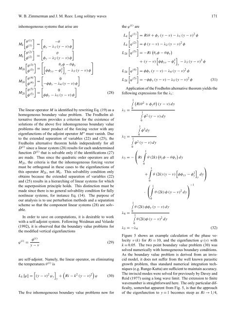Figure 5 shows an example calculation of the phase velocity ν (k) for Ri = 10, and the eigenfunction ϕ (y) with k = 0.05. The two point boundary value problem (30) was solved numerically with homogeneous boundary conditions. As the boundary value problem is derived from an inviscid model, it does not suffer from the well known parasitic growth problem, thus standard numerical integration techniques (e.g. Runge-Kutta) are sufficient to maintain accuracy. The inviscid modes were solved for previously by Davey and Reid (1977) using a long wave limit. The extension to finite wavenumber is straightforward here. The only particular difficulty, somewhat apparent from Fig. 5, is that the approach of the eigenfunction to y = 1 becomes steep as Ri → 1/4, −1
Page 1 and 2: Nonlinear Processes in Geophysics (
Page 3 and 4: W. B. Zimmerman and J. M. Rees: Lon
Page 5: W. B. Zimmerman and J. M. Rees: Lon

Long solitary internal waves in stable stratifications

Create successful ePaper yourself

Delete template?

Save as template?