Full Wave Form Inversion for Seismic Data

Full Wave Form Inversion for Seismic Data KSG 2011 

Full Wave Form Inversion for Seismic Data 

Problem presented by 

Tong Fei 

Saudi Aramco 

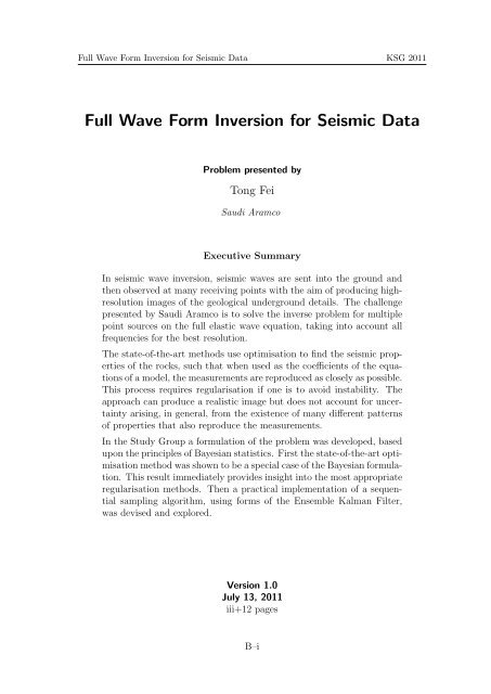
Executive Summary 

In seismic wave inversion, seismic waves are sent into the ground and 

then observed at many receiving points with the aim of producing highresolution 

images of the geological underground details. The challenge 

presented by Saudi Aramco is to solve the inverse problem for multiple 

point sources on the full elastic wave equation, taking into account all 

frequencies for the best resolution. 

The state-of-the-art methods use optimisation to find the seismic properties 

of the rocks, such that when used as the coefficients of the equations 

of a model, the measurements are reproduced as closely as possible. 

This process requires regularisation if one is to avoid instability. The 

approach can produce a realistic image but does not account for uncertainty 

arising, in general, from the existence of many different patterns 

of properties that also reproduce the measurements. 

In the Study Group a formulation of the problem was developed, based 

upon the principles of Bayesian statistics. First the state-of-the-art optimisation 

method was shown to be a special case of the Bayesian formulation. 

This result immediately provides insight into the most appropriate 

regularisation methods. Then a practical implementation of a sequential 

sampling algorithm, using forms of the Ensemble Kalman Filter, 

was devised and explored. 

Version 1.0 

July 13, 2011 

iii+12 pages 

B–i


Report coordinator 

C. Farmer, I. Hoteit, X. Luo, C. Boonyasiriwat and T. Alkhalifah 

Contributors 

Tariq Alkhalifah (KAUST, Saudi Arabia) 

Mohammed Alsunaidi (KFUPM, Saudi Arabia) 

Chaiwoot Boonyasiriwat (KAUST, Saudi Arabia) 

Nadia Chouaieb (KAUST, Saudi Arabia) 

R. Djebbi (KAUST, Saudi Arabia) 

Shouhong Du (KAUST, Saudi Arabia) 

Chris Farmer (OCCAM, UK) 

Nicholas Hale (OCCAM, UK) 

Ibrahim Hoteit (KAUST, Saudi Arabia) 

Taous-Meriem Laleg-Kirati (KAUST, Saudi Arabia) 

Chong Luo (OCCAM, UK) 

Xiaodong Luo (KAUST, Saudi Arabia) 

Alvaro Moraes (KAUST, Saudi Arabia) 

Surya Pachhai (KAUST, Saudi Arabia) 

Pedro Vilanova (KAUST, Saudi Arabia) 

Babar Hasan Khan (KAUST, Saudi Arabia) 

Pedro Guerra (KAUST, Saudi Arabia) 

Abdulrahman Al-shuhail (KAUST, Saudi Arabia) 

Mohamad Elgharamti (KAUST, Saudi Arabia) 

KSG 2011 was organised by 

King Abdullah University of Science and Technology (KAUST) 

In collaboration with 

Oxford Centre for Collaborative Applied Mathematics (OCCAM) 

B–ii


Contents 

1 Introduction 1 

2 Forward Problem 3 

2.1 Continuum forward model . . . . . . . . . . . . . . . . . . . . . . . 3 

2.2 Discrete forward model . . . . . . . . . . . . . . . . . . . . . . . . . 4 

3 Minimum Misfit Formulation of the Inverse Problem 5 

4 Inverse Problems from the Statistical Viewpoint 6 

4.1 The Sequential Bayesian Filtering Equations . . . . . . . . . . . . . 6 

4.2 The Bayesian Smoothing Equation . . . . . . . . . . . . . . . . . . 7 

5 Practical Methods for Implementing a Bayesian Filter 8 

6 Conclusions 10 

Bibliography 11 

B–iii


1 Introduction 

Saudi Aramco is an oil company responsible for the discovery and recovery of hydrocarbons 

from geological formations. The principal method for the exploration 

of oil is the seismic survey. 

Seismic acquisition involves sending acoustic energy into the subsurface and 

analysing the echoes. This is an inverse problem on the acoustic or even the full 

elastic wave equation. Data are gathered from many independent experiments, as a 

sound source is activated in a sequence of shots as it is moved over the land or sea 

surface. The results are preprocessed using a wide range of techniques designed to 

correct for topographical features and noise. A complete review of these techniques 

can be found in [12]. 

Figure 1: A schematic cross-section of a complex geological pattern and a seismic shot. 

After preprocessing, and in a traditional workflow, the main inversion step is 

known as migration. The amount of data, and the size of the system under investigation 

are both very large. Until recently this precluded the use of simple 

numerical techniques for solving the forward model, as used for example for the 

fluid flow forward problem when performing oil reservoir simulation. Instead a 

range of semi-analytical approximations are used in routine applications. The approximations 

vary in accuracy, complexity and applicability. The simplest methods 

are known as time migration, using the Born approximation obtained from linearisation 

about a simple background spatial distribution of elastic properties. The Born 

approximation is solved using Fourier methods. For a detailed explanation of the 

mathematical theory see [2]. In recent years more sophisticated and more accurate 

methods known as depth migration based on high-frequency ray-tracing methods 

have been developed. However, with the continuing rapid increases in computing 

resources, it is now becoming possible to use full finite difference or pseudo-spectral 

approximations. The resolution requirements are very demanding and it can take 

many millions of computing hours to obtain a single inversion, but the prospects 

that full inversion provides make this a valuable topic for further research. 

B–1


The results are usually presented in the time domain which, to a first approximation, 

removes the effects of any layer cake background model. Users of the inverted 

results are able to apply their own time-to-depth conversions as more data becomes 

available, or as the seismic data is combined with other data. The time-to-depth 

conversion is performed using alternative layer cake models of the sound speed and 

rock density. Note that depth processed seismic results using depth migration are 

often displayed in the time domain by applying a depth-to-time conversion. 

After migration, and display in the time domain, the observations are equivalent 

to a numerical experiment that measures the response that would be observed in 

an ideal experiment where the sound waves are assumed to propagate in vertical, 

straight lines, and that any reflectors that are encountered are locally horizontal. 

The resulting calculations are then displayed as seismograms of the virtual experiment. 

At the Study Group, Tong Fei of Saudi Aramco explained how full wave form 

inversion (FWI), as the rigorous solution of the inverse problem for wave propagation 

is known, holds out the prospect of improved quality of the seismic images 

enabling the recovery of oil from geological formations with greater reliability than 

more traditional approaches. 

The FWI method currently used by Saudi Aramco, other oil companies and 

many academic researchers is to formulate the inverse problem in the usual ‘minimum 

misfit with regularisation’ framework. That is, the solution of the forward 

problem is re-cast as an equation that predicts the measurements if the rock properties 

were known. The properties are then adjusted until the predicted measurements 

match the actual measurements. Such a process is generally ill-posed in that 

there are many geometric arrangements of properties that provide a good match 

(although very hard to compute) and further a small change in the values of the 

measurements or the details of the forward model can give rise to a large change in 

the properties that provide the match. For this reason additional terms have to be 

added to the misfit function to remove the instability. However, such a process does 

not remove the non-uniqueness. Saudi Aramco were using the method of first order 

Tikhonov regularisation which stabilises the misfit function by adding a weighted 

sum of squares of the physical properties as averaged over a grid cell. 

In the Study Group the discussion turned to the application of statistical ideas 

to the inverse problem. The academic participants first of all explained how to 

interpret the Tikhonov approach as the negative logarithm of a prior probability 

density function representing the prior geological knowledge. Then they worked on 

ways of reducing the complexity of the Bayesian approach so that the uncertainty 

could be properly quantified and calculations representing the full posterior density 

function could be performed with a level of computation similar to that of the less 

complete deterministic regularised minimum misfit approach. 

The Study Group performed some simple numerical experiments which appeared 

to indicate that progress might be possible. However, the problem is exceedingly 

difficult and so the group concentrated on the formulation of the problem and the 

groundwork needed for others to make a later proposal for further research. 

The following report outlines the background knowledge required to understand 

B–2


where s is the source term and c p is the speed of ‘P-waves’ such that c p = (λ+2µ)/ρ. 

By taking the curl of the Navier equations one obtains a linear wave equation 

for a vector field of shear waves, called ‘S-waves’, that travel with a local speed of 

c s = µ/ρ. Generally the P-waves travel at a faster speed than the S-waves and 

in many approaches to seismic exploration theory it is only the P-waves that are 

modelled. However, in more recent literature there is a growing interest in using 

the full Navier equation or even the full elasto-dynamic equations with only some 

assumptions of material symmetry appropriate, for example, for a layered material. 

2.2 Discrete forward model 

The standard and most straightforward method for solving the various wave equations 

is to use a finite difference method. Saudi Aramco have been using very 

high order methods, as high as 12-th or 14-th order. We will not describe the details 

of this, as this was not discussed during the Study Group and is not key to 

understanding the inverse problem. 

Let us suppose that time is discretised into discrete times t n , with n = 0, 1, ... 

and such that the response is observed at each t n and the shots occur at sporadic 

times, with many time steps in between. When solving the discretised wave equation 

there might well be many subsidiary time steps, for reasons of numerical stability or 

accuracy, in between the observation times. The measurements themselves might 

be averaged or interpolated so that the model discrete time, the observation times, 

and the times at which shots are fired are co-ordinated. 

Thus let us model the state of the sub-surface by a finite vector of values, ψ t . 

The components of ψ t might be Fourier amplitudes or the values at grid points or 

averages over grid cells. The properties, also represented by Fourier amplitudes or 

grid point values, are a finite vector of values m. 

At each observation time step, the causal nature of the underlying wave equations 

implies that Earth’s seismic state at t+1 is a known function g t of the state at 

time-t. This function is computed via the numerical solution of the wave equation, 

and can be written as: 

ψ t+1 = g t (ψ t , m) (6) 

As the initial dynamical state of Earth, just before the first shot is known, the state 

at time-1 is given by ψ 1 = g 1 (ψ 0 , m). We note that ψ 0 is a known quantity as Earth 

is stationary before the first shot, as indeed it will be just before each shot (unless 

the shots were made so rapidly that the reverberations from the previous shot have 

not yet dissipated). 

The measurements at the receivers are modelled in a fairly general case by the 

expression: 

d t = h(ψ t ) + ζ t (7) 

where ζ t is Gaussian noise with variance σ. It is quite common to assume that the 

noise is Gaussian as this is thought to be a generally good model, and simplifies 

subsequent calculations. However, if this is not a good model one can transform 

the variables so that the noise can be Gaussian and one can even assume that all 

B–4


measurement operators are linear if extra variables are introduced. (For details see 

the paper [13].) 

It then follows that the measurements are modelled by the equation: 

d t = G t (m) + ζ t (8) 

where G t is a function obtained by induction using the function g t . For example 

G 2 (m) = g 2 (g 1 (ψ 0 , m))). The last equation shows that we can consider the 

predictions of the measurements as known functions of the properties m. 

The different positions of each of the shots are modelled implicitly in the form 

of the model function g t . Note that shots are not fired at all times, indeed only at a 

very small number of times. Also in practice, just before the shot is made one can 

assume that Earth is stationary, so that the dynamic parameters are always known 

at the time just before the shot, but because Earth’s material properties are not 

known the state of Earth is not known during the time after the shot when Earth is 

reverberating with the seismic waves. The only information that is known for sure 

is the set of values of the measurements. 

3 Minimum Misfit Formulation of the Inverse Problem 

To formulate the inverse problem as an optimisation problem, one first forms the 

data vector D n = {d 1 , ..., d n }. One can then form the function 

C(m) = 1 ∑ 

(d n − G n (m)) T W d (d n − G n (m)) + 1 2 

2 ɛ(m − m p) T W m (m − m p ) (9) 

n 

where W d = δ i,j /σ 2 is the inverse correlation matrix of the (white) Gaussian measurement 

noise and W m the inverse correlation matrix for the regularisation terms. 

It is, apparently, quite usual to assume that W m is the identity matrix δ i,j which 

gives rise to zeroth-order Tikhonov regularisation. The parameter, ɛ is somewhat 

problematic in the regularisation framework. The standard approach for choosing 

the size of ɛ is the ‘discrepancy principle’ whereby one chooses the parameter so 

that the magnitude of the total misfit function is of the order of the magnitude 

of the measurement errors. This is explained fully in the book [9]. The Bayesian 

framework, however, provides clear guidance on how to choose ɛ. 

The minimum misfit method seeks a property vector m to minimise the function 

C(m) using a gradient optimisation method. Computation of the gradient requires 

computation of the derivative of the misfit function C(m). In general the misfit 

function does not have a unique minimum so a decision procedure or some way 

of weighting the minima is required. Suppose that all of the minima are different 

from one another. Then one way of providing a decision procedure is to ask for 

the global minimum (that local minimum that is lower than all of the other local 

minima). However, finding global minima is generally an expensive process and in 

many cases infeasible. Further, if we fail to find the global minimum then numerical 

B–5


experiments (for example see the paper [3]) show that some local minima that are 

lower than many other local minima are, nevertheless, worse predictors than their 

higher cousins. If we add to this observation the thought that the original forward 

model that we have chosen will always be imperfect in some way or other, then the 

minimum misfit method can be seen to be dangerous and misleading unless there are 

very good reasons to suppose otherwise. For example if the misfit function is known 

to have a unique minimum and the misfit function has a large second derivative at 

the minimum, then the properties at this minimum may be a reasonable estimate 

of the true properties. Theoretical considerations lead to such a conclusion as the 

situation corresponds to a Gaussian posterior density with a small variance. 

A particularly relevant review of the minimum misfit approach to the FWI 

problem can be found in reference [15]. 

We now outline the statistical approach which promises to alleviate these difficulties 

of the minimum misfit method. However we will see that new difficulties 

arise. 

4 Inverse Problems from the Statistical Viewpoint 

4.1 The Sequential Bayesian Filtering Equations 

In the statistical approach one summarises all of one’s prior knowledge - before any 

seismic measurements are made - by a probability density function of the properties, 

π 0 (m). The idea of this is that any particular realisation from the prior will, 

when visualised, ‘look’ like a typical geology of the type we imagine to be under 

investigation. The company geologists are the primary drivers of this, and will use 

their collective expertise to devise a prior that is a satisfactory representation of 

their geological intuitions and is conditioned on any available data such as logs from 

existing wells. Of course, in the actual company workflow previous seismic surveys 

will be available and this information is important in building the best possible 

prior. Note however, that the quality of a prior can be considered to be the quality, 

alone, of how well the prior represents the prior knowledge. The quality of the 

prior knowledge of itself, can be considered a separate matter, although of equal 

importance. It is useful in discussions and in writing to separate considerations of 

the quality of representation of knowledge from the quality of the knowledge itself. 

This is true also of the posterior density. The quality (or more clearly the accuracy) 

with which the posterior has been calculated as a consequence of the model, 

the prior and the quantity and quality of the measurements is a separate matter 

from the quality (accuracy) of the model, of the prior and of the relevance of the 

measurements. Failure to make these distinctions is confusing and can lead us into 

error. It is quite common to evaluate the quality of a forecasting or data assimilation 

system by evaluating the posterior density with respect to the ‘truth’ in some 

ideal numerical experiment. Such experiments are not useful unless a very accurate 

calculation (or even an exact calculation) of the posterior density is available with 

which to compare the results. 

The Bayesian approach takes the view that the prior at time-0 is the starting 

B–6


point for subsequent assimilation of the data into our knowledge. The process is 

quite simple. Thus assume that at time-t we have already calculated π t (ψ t , m|D t ). 

That is, the latest probability density function of the static properties, m and the 

dynamical state ψ t , conditional upon all of the measurements up to, and including 

those at time-t. Then, by application of the principles of probability theory, we 

can write down the joint density of the current state, the next state and the next 

measurements (before they are made). This is: 

π(d t+1 , ψ t+1 , m|D t ) = π σt (d t+1 − h(ψ t+1 ))δ(ψ t+1 − g(ψ t ))π t (ψ t , m|S t ) (10) 

where δ(.) is the delta measure that is appropriate for a forward model without any 

dynamical noise. 

By integrating out the earlier dynamical state, and by normalising the equations 

(that is, by using Bayes’ theorem) the posterior probability density for the states 

and properties is given by the expression: 

∫ 

π(ψ t+1 , m|D t+1 ) = z t+1 π σ (d t+1 − h(ψ t+1 )) δ(ψ t+1 − g(ψ t ))π t (ψ t , m|D t )dψ t (11) 

where z t+1 is a normalisation constant required so that the posterior density integrates 

to unity. We note that the great difficulty of the Bayesian approach is, in 

general, in performing this high dimensional integration at each time step. 

Thus, from the prior at t = 0, a sequential application of equation(11) enables 

us, in principle to compute the posterior density functions at each time. 

4.2 The Bayesian Smoothing Equation 

From the iterated form of the forward model we can write down the posterior density 

of the static properties alone by the expression: 

π(m|D t ) = Z t Π n π σ (d n − G n (m)))π 0 (m) (12) 

where the product Π n ranges from n = 1 to n = t. This is known as the ‘smoothing 

equation’ as the pdf of the properties depends upon all of the measurements. We 

note that the pdf in this formula is identical to the marginal pdf that would be obtained 

from the filtering equations of the previous section once we have marginalised 

the posterior density by integrating out the dynamical state. It is noted that the filtering 

equations are known as such, because the marginal density of the dynamical 

state at any particular time does not depend upon observations at later times. 

A natural method of summarising this joint posterior probability density is to 

seek the properties, m that maximise the value of π(m|D t ). This is equivalent to 

taking the negative logarithm and seeking the minimum. Thus taking the logarithm 

of equation(12) gives the expression; 

C(m) = − log π(m|D t ) = − log Z t + ∑ n 

1 

2σ 2 (d n − G t (m)) 2 − log π 0 (m) (13) 

We can see from the last equation, that except for the constant, this is the 

same form as the equation for the minimum misfit method. By taking the prior 

B–7


to be the exponential of minus the regularisation term we have shown that the 

regularisation is equivalent to a particular prior probability density. In the book of 

[14] the advice is given that one should always use a Monte-Carlo sampling method 

to draw realisations from the prior to see if, when they are visualised, they conform 

to the prior judgements of the company geologists as to the texture of the rocks 

of interest. The various Tikhonov priors do not always correspond to well defined 

pdf’s. However, the zeroth-order Tikhonov regularisation does correspond to such 

a pdf and is the pdf for ‘white noise’. This is a noise with zero correlation length 

and when visualised looks completely isotropic and like fine gravel or sand. This 

may be appropriate, or on the other hand it might not be appropriate. For further 

discussion of the link between Tikhonov regularisation and Gaussian priors see the 

book of [14] or the article [5]. 

5 Practical Methods for Implementing a Bayesian 

Filter 

Thus there are good theoretical grounds for the view that an inverse problem is 

solved once one has computed the posterior probability density. However in practice 

this is just the beginning. The first problem is to represent the pdf’s in some way, 

and the next problem is to perform the high dimensional integration at each time 

step. The first practical problem is approached using an ensemble representation. 

That is, if we have an ensemble of size R of equal weight realisations {ψ r t} R r=1 we 

can recover an estimate of the pdf from the expression 

π(ψ t |D t ) = 1 ∑ 

δ(ψ t − ψ r t ) (14) 

R 

Using this expression in the filtering equations makes it easy to perform the integral; 

once anyway. The next difficulty is that the weights in the subsequent expressions 

are no longer the same as each other. This makes it necessary to add an extra step 

in which the realisations are modified so that they are equal weight realisations. 

The different ways of doing this give rise to the different varieties of filtering. Many 

of the methods that have been used try to employ ideas from the Kalman Filter. 

The forward model for a linear system is of the form. 

r 

ψ t+1 = A t ψ t + B t m + ξ t (15) 

where A t and B t are known matrices and ξ t is a random Gaussian vector with zero 

mean and known correlation structure. Further the observation model is also linear, 

d t = Hψ t + ζ t (16) 

where H t is a known matrix. 

In the case of a linear forward model with a linear observation model, with a 

Gaussian prior at the initial time and with Gaussian noise, the posterior density is 

always Gaussian. Thus we can compute the posterior mean and correlation matrix, 

B–8


Figure 2: An illustration of the EnKF for a two-component time dependent state. 

conditioned on all of the observations up to the current time. This is the Kalman 

filter. The equations are quite complicated, but the derivation follows from the 

assumptions just stated. (For a particularly clear derivation, see the book [11].) 

When the dimension of the state vector is very large, the Kalman filter, even 

given the validity of the assumptions (which is not very usual), the algorithm is 

impractical because the dimension of the various matrices used in the calculations 

is too large. A recent development is the Ensemble Kalman filter, which by representing 

the Gaussian pdf by an ensemble, can circumvent the problem related to 

the size of matrices. This is a consequence of the natural way in which the ensemble 

correlation matrix is naturally factorised by the ensemble members. It can be shown 

(see [4]) that the Ensemble Kalman Filter (EnKF) converges to the exact answer 

for the linear and Gaussian case. This is a very significant advance and leads us 

to believe that soon it will be possible to solve most large scale inverse problems 

in a fairly routine manner. However it is unfortunately not a panacea, as very few 

problems are linear and Gaussian. There is still a great deal of research to be done 

to fulfill the promise given by the EnKF. 

However, in the current state of the art, the Ensemble Kalman Filter described 

in detail in [4] provides one of the most popular and successful ensemble inversion 

methods. We do not give the details here, but we do record that the academic 

participants at the KAUST Study Group recommended that as a first step in any 

further work a form of the Ensemble Kalman Filter should be tried on the problem 

of FWI. We note, that the Ensemble Kalman Filter uses some of the equations of 

the Kalman filter in the update step. Thus the method is not rigorous, and does 

not converge in the limit of increasing ensemble size. There are newer methods that 

are convergent, and these methods are likely to supersede the EnKF. At the present 

time there is a great deal of activity in the field and it is not yet possible to say 

which method (or methods) will come to dominate the subject. 

B–9


In figure 2 we indicate how, at time-t a well-constructed ensemble - shown by 

the blue dots - will surround the state of reality as shown by the green dot. When 

the forward model updates the posterior at time-t to the prior at time-(t + 1) we 

see that if the forward model is adequate it will, once again surround the state of 

reality. Then we see that, in the case where the measurements do actually carry 

some new information, that the variance of the posterior ensemble (shown by the 

orange dots) is smaller than the variance of the prior ensemble. We note that over 

many time steps, as a result of natural and computational fluctuations, sometimes 

the real state is in the tails of the prior. However, in general, if the posterior density 

at time-t is always very different from the prior at time-t at many different times 

then we must suspect that the forward model needs to be improved. This is how 

model validation can be built into the Bayesian framework in a natural way. 

6 Conclusions 

At the Study Group, once it was realised that the FWI seismic inversion problem 

could be formulated as a sequential filtering problem, in the natural way that the 

actual seismic data gathering process suggests, the participants were very keen to 

try the idea. A one dimensional scalar wave equation was used in a simple example. 

Using code provided by Chaiwoot Boonyasiriwat (KAUST) the forward problem 

was solved. Also the code from Chaiwoot was able to solve the inverse problem 

using a minimum misfit approach. Then using a version of the Ensemble Kalman 

filter provided by Xiaodong Luo (KAUST) the inverse problem was solved. At the 

time of the Study Group, when we presented in the final plenary session, we had 

not fully analysed our results, and the presentation gave the impression that we 

had succeeded in solving the problem using the EnKF. However, after the meeting, 

with some more analysis, we realised that the results were not as decisive as we 

had first thought, and it is now apparent that a more powerful, fully nonlinear 

filtering method is required. Although the the minimum misfit approach was able 

to retrieve a good estimate of the unobserved rock parameters in the test problem 

is still remains the case that the minimum misfit method is unable to quantify the 

uncertainty in the retrieved model. 

After discussing the results further, we realised that the Ensemble filtering 

method that we used at the time of the Study Group involved assumptions of 

linearity and Gaussianity which are not valid. As mentioned in the previous sections, 

the standard methods of Bayesian filtering, as in the Ensemble Kalman Filter, 

make essential use of assumptions of linearity in the model and Gaussianity in the 

error statistics. More recent work such as that of [6] and [7] and the work [13] show 

that these assumptions can be removed. 

We thus recommend that more work should be done where the newer 

and rigorous filtering methods are used. Perhaps, the EnKF and, of 

course, the minimum misfit methods could be used as benchmarks. The 

principal authors of this report are of the view that these methods are 

likely to succeed. However, this is a very challenging problem, but the 

rewards of a successful result will be very high. 

B–10


Bibliography 

[1] K. Aki and P. G. Richards, Quantitative Seismology. University Science 

Books, Sausilito, California, 2002. 

[2] N. Bleistein, J. K. Cohen and J. W. Stockwell, Jr., Mathematics of 

Multidimensional Seismic Imaging, Migration and Inversion. Springer-Verlag, 

New York, USA, 2001. 

[3] J. N. Carter, P. J. Ballestera, Z. Tavassolia and P. R. 

King., Our Calibrated Model has No Predictive Value: An Example 

from the Petroleum Industry. Preprint, available from: 

http://www3.imperial.ac.uk/pls/portallive/docs/1/39240.PDF 

[4] G. Evensen., Data assimilation, The Ensemble Kalman Filter, 2nd ed. 

Springer-Verlag, Heidelberg, 2009. 

[5] C. L.Farmer, Bayesian Field Theory Applied to Scattered Data Interpolation 

and Inverse Problems. Algorithms for Approximation. Ed. A. Iske and J. 

Levesley, Springer-Verlag, Heidelberg, 2007, pp. 147-166. 

[6] I. Hoteit, D. -T. Pham, G. Korres and G. Triantafyllou., Particle 

Kalman filtering for data assimilation in meteorology and oceanography. In: 

3rd WCRP International Conference on Reanalysis, p. 6. Tokyo, Japan, 2008. 

[7] I. Hoteit, D. -T. Pham, G. Triantafyllou and G. Korres., A new 

approximative solution of the optimal nonlinear filter for data assimilation in 

meteorology and oceanography. Mon. Weather Rev. 136, 317334, 2008. 

[8] P. Howell, G. Kozyreff and J. Ockendon, Applied Solid Mechanics. 

Cambridge University Press, Cambridge, UK, 2009. 

[9] J. Kaipio and E. Somersalo, Statistical and Computational Inverse Problems. 

Springer-Verlag, New York, 2004. 

[10] G. Nolet, A Breviary of Seismic Tomography: Imaging the Interior of the 

Earth and Sun. Cambridge University Press, Cambridge, UK, 2008. 

[11] C. D. Rodgers, Inverse Methods for Atmospheric Sounding: Theory and 

Practice. World Scientific Publishing Co. Ltd., 2000. (Reprinted with corrections, 

2008). 

[12] R. E. Sheriff and L. P. Geldart, Exploration Seismology. Cambridge 

University Press, Cambridge, UK, 1995. 

[13] A. S. Stordal, H. A. Karlsen, G. Nævdal, H. J. Skaug, and 

B. Vallès, Bridging the ensemble Kalman filter and particle filters: the 

adaptive Gaussian mixture filter. Computational Geosciences, 2010, DOI 

10.1007/s10596-010-9207-1. 

B–11


[14] A. Tarantola, Inverse Problem Theory and Methods for Model Parameter 

Estimation. SIAM, Philadelphia, USA, 2005. 

[15] J. Virieux and S. Operto, An overview of full-waveform inversion in exploration 

geophysics Geophysics, 2009, Vol. 74, No. 6 November-December. 

B–12

Full Wave Form Inversion for Seismic Data

You also want an ePaper? Increase the reach of your titles

Delete template?

Save as template?