Identification of the parameters of the Kelvin–Voigt and the Maxwell ...
Identification of the parameters of the Kelvin–Voigt and the Maxwell ...
Identification of the parameters of the Kelvin–Voigt and the Maxwell ...

Create successful ePaper yourself
Turn your PDF publications into a flip-book with our unique Google optimized e-Paper software.
ARTICLE IN PRESS<br />
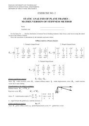
2 R. Lew<strong>and</strong>owski, B. Chorą_zyczewski / Computers <strong>and</strong> Structures xxx (2009) xxx–xxx<br />
<strong>the</strong> <strong>Maxwell</strong> ladder is presented in [6]. Moreover, <strong>the</strong> non-viscous<br />
state-space model, described in [31], could be used in this context.<br />
The analysis in <strong>the</strong> frequency domain is possible <strong>and</strong> presented, for<br />
example, in [3].<br />
An important problem, connected with <strong>the</strong> fractional rheological<br />
models, is an estimation <strong>of</strong> <strong>the</strong> model <strong>parameters</strong> from experimental<br />
data. In <strong>the</strong> past, different methods have been tested for<br />
<strong>the</strong> estimation <strong>of</strong> model <strong>parameters</strong> from both static <strong>and</strong> dynamic<br />
experiments [4,8,9,16–19,21]. The process <strong>of</strong> parameter identification<br />
is an inverse problem which is overdetermined <strong>and</strong> can be ill<br />
conditioned (see, for example [8,19]) because <strong>of</strong> noises existing in<br />
<strong>the</strong> experimental data. The ma<strong>the</strong>matical difficulties may be overcome<br />
by <strong>the</strong> regularization method which is described, for example,<br />
in [8,18].<br />
It is <strong>the</strong> aim <strong>of</strong> this paper to describe a few methods <strong>of</strong> identification<br />
<strong>of</strong> <strong>the</strong> <strong>parameters</strong> <strong>of</strong> VE dampers. The <strong>parameters</strong> are estimated<br />
using <strong>the</strong> results obtained from dynamical tests. The<br />
fractional rheological models are used to describe <strong>the</strong> dynamic<br />
behaviour <strong>of</strong> dampers. The Kelvin–Voigt model <strong>and</strong> <strong>the</strong> <strong>Maxwell</strong><br />
model are discussed. Three kinds <strong>of</strong> identification methods are suggested.<br />
Equations <strong>of</strong> hysteresis curves are derived for both fractional<br />
models <strong>and</strong> some <strong>of</strong> <strong>the</strong> properties <strong>of</strong> <strong>the</strong>se curves are<br />
used to develop <strong>the</strong> first-kind identification procedure. The second-<br />
<strong>and</strong> third-kind identification procedures are based on time<br />
series data. Each identification procedure consists <strong>of</strong> two main<br />
steps. In <strong>the</strong> first step, for <strong>the</strong> given frequencies <strong>of</strong> excitation,<br />
experimentally obtained data are approximated by simple harmonic<br />
functions while model <strong>parameters</strong> are determined in <strong>the</strong><br />
second stage <strong>of</strong> <strong>the</strong> identification procedure. The results <strong>of</strong> a typical<br />
calculation are presented <strong>and</strong> discussed.<br />
Three symbols will be used in <strong>the</strong> paper to describe <strong>the</strong> damper<br />
force. The symbol u e ðtÞ denotes <strong>the</strong> results <strong>of</strong> experimental measurements,<br />
~uðtÞ is <strong>the</strong> function which is an analytical approximation<br />
<strong>of</strong> experimental results while uðtÞ is <strong>the</strong> solution to <strong>the</strong><br />
damper equation <strong>of</strong> motion. The symbols q e ðtÞ; ~qðtÞ <strong>and</strong> qðtÞ are<br />
used in <strong>the</strong> same way to describe <strong>the</strong> damper displacement.<br />
2. General explanation <strong>of</strong> fractional rheological models<br />
Due to <strong>the</strong>ir simplicity, <strong>the</strong> simple rheological models, such as<br />
<strong>the</strong> Kelvin–Voigt model or <strong>the</strong> <strong>Maxwell</strong> model, are used very <strong>of</strong>ten<br />
to describe <strong>the</strong> dynamic behavior <strong>of</strong> VE dampers installed on<br />
various types <strong>of</strong> civil structures. For example, <strong>the</strong> Kelvin–Voigt<br />
model is used in papers [2,3,22–24], while <strong>the</strong> <strong>Maxwell</strong> model<br />
is used in papers [2,3,25–28]. The Kelvin–Voigt model consists<br />
<strong>of</strong> <strong>the</strong> spring <strong>and</strong> <strong>the</strong> dashpot connected in parallel, while <strong>the</strong><br />
<strong>Maxwell</strong> model is built from <strong>the</strong> serially connected spring <strong>and</strong><br />
dashpot. The discussed simple rheological models have a small<br />
number <strong>of</strong> <strong>parameters</strong> but do not have enough <strong>parameters</strong> to<br />
accurately capture <strong>the</strong> frequency dependence <strong>of</strong> damper <strong>parameters</strong>.<br />
More sophisticated classical rheological models which, however,<br />
contain many <strong>parameters</strong>, can be used to correctly describe<br />
<strong>the</strong> dynamic behavior <strong>of</strong> VE dampers. Models <strong>of</strong> this kind are<br />
developed in [6,7].<br />
The next group <strong>of</strong> models used to describe <strong>the</strong> behaviour <strong>of</strong> VE<br />
dampers are <strong>the</strong> fractional derivative models. Using <strong>the</strong> fractional<br />
calculus, a number <strong>of</strong> rheological models, e.g., <strong>the</strong> fractional Kelvin–Voigt<br />
model [32], <strong>the</strong> fractional Zener model [10,11], <strong>the</strong> fractional<br />
Jeffreys model [12], or <strong>the</strong> fractional <strong>Maxwell</strong> model [17] can<br />
be developed. It has been proved in [4,15] that <strong>the</strong> fractional derivative<br />
models can better capture <strong>the</strong> frequency dependent properties<br />
<strong>of</strong> VE dampers. The simple fractional models discussed in<br />
[4,13,15] are sufficient to correctly capture <strong>the</strong> VE dampers properties.<br />
These models contain only a few <strong>parameters</strong> but <strong>the</strong> dynamic<br />
analysis requires knowledge <strong>of</strong> <strong>the</strong> fractional calculus.<br />
The simple Kelvin–Voigt model seems to be more appropriate<br />
to describe <strong>the</strong> solid dampers behavior, while <strong>the</strong> simple <strong>Maxwell</strong><br />
model is mainly used to describe <strong>the</strong> liquid dampers behavior. Recently,<br />
it has been shown in [6] that both <strong>the</strong> generalized Kelvin<br />
model <strong>and</strong> <strong>the</strong> generalized <strong>Maxwell</strong> model are also useful models<br />
<strong>of</strong> <strong>the</strong> solid VE damper.<br />
One important problem, considered here <strong>and</strong> connected with<br />
<strong>the</strong>se models, is how to determine model <strong>parameters</strong> from experimental<br />
data in an efficient way. This problem is solved in this Section<br />
for <strong>the</strong> fractional Kelvin–Voigt model <strong>and</strong> <strong>the</strong> fractional<br />
<strong>Maxwell</strong> model.<br />
2.1. Fractional models equation <strong>of</strong> motion <strong>and</strong> <strong>the</strong> steady state solution<br />
to <strong>the</strong> motion equation<br />
In order to construct <strong>the</strong> fractional models equation <strong>of</strong> motion,<br />
we introduce <strong>the</strong> fractional element called <strong>the</strong> springpot which<br />
satisfies <strong>the</strong> constitutive equation:<br />
uðtÞ ¼~c a D a t qðtÞ ¼cDa t qðtÞ;<br />
where c ¼ ~c a <strong>and</strong> a; 0 < a 6 1, are <strong>the</strong> springpot <strong>parameters</strong> <strong>and</strong><br />
D a t<br />
qðtÞ is <strong>the</strong> fractional derivative <strong>of</strong> <strong>the</strong> order a with respect to time<br />
t. There are a few definitions <strong>of</strong> fractional derivatives which coincide<br />
under certain conditions. Here, symbols such as D a t<br />
qðtÞ denote<br />
<strong>the</strong> Riemann–Liouville fractional derivatives with <strong>the</strong> lower limit at<br />
– 1 (see [34]). Some valuable information about fractional calculus<br />
can be found in [34].<br />
The springpot element, also known as <strong>the</strong> Scott–Blair’s element<br />
(see [33]), is schematically shown in Fig. 1a. The considered element<br />
can be understood as an interpolation between <strong>the</strong> spring<br />
element ða ¼ 0Þ <strong>and</strong> <strong>the</strong> dashpot element ða ¼ 1Þ.<br />
The fractional Kelvin–Voigt model consists <strong>of</strong> <strong>the</strong> spring<br />
<strong>and</strong> <strong>the</strong> springpot connected in parallel, while <strong>the</strong> fractional<br />
<strong>Maxwell</strong> model is built <strong>of</strong> <strong>the</strong> serially connected spring <strong>and</strong> springpot.<br />
These models are shown schematically in Fig. 1b <strong>and</strong> c,<br />
respectively.<br />
The motion equation <strong>of</strong> <strong>the</strong> above mentioned fractional Kelvin–<br />
Voigt model, obtained in a usual way, is in <strong>the</strong> following form:<br />
uðtÞ ¼kqðtÞþks a D a t qðtÞ;<br />
where s a ¼ ~c a =k ¼ c=k.<br />
The following relationships can be written for <strong>the</strong> fractional<br />
<strong>Maxwell</strong> model (Fig. 1c)<br />
uðtÞ ¼kq 1 ðtÞ; uðtÞ ¼~c a D a t ðqðtÞ q 1ðtÞÞ: ð3Þ<br />
Eliminating q 1 ðtÞ from <strong>the</strong> above relationships, we get <strong>the</strong> equation<br />
in <strong>the</strong> form:<br />
uðtÞþs a D a t uðtÞ ¼ksa D a t qðtÞ:<br />
ð4Þ<br />
It is easy to recognize that both <strong>of</strong> <strong>the</strong> considered fractional models<br />
have three real <strong>and</strong> positive value <strong>parameters</strong>: k, c, <strong>and</strong> a.<br />
In <strong>the</strong> case <strong>of</strong> a harmonically excited damper, i.e. when<br />
qðtÞ ¼q 0 expðiktÞ;<br />
<strong>the</strong> steady state solution <strong>of</strong> <strong>the</strong> motion equation <strong>of</strong> both <strong>of</strong> <strong>the</strong> fractional<br />
models is assumed in <strong>the</strong> form:<br />
uðtÞ ¼u 0 expðiktÞ:<br />
Taking into account that in our case (see [34, p. 311])<br />
D a t expðiktÞ ¼ðikÞa expðiktÞ;<br />
for k > 0, we obtain <strong>the</strong> following equations<br />
u 0 ¼ k½1 þðiskÞ a ðiskÞ a<br />
Šq 0 ; u 0 ¼ k<br />
1 þðiskÞ a q 0 ; ð8Þ<br />
ð1Þ<br />
ð2Þ<br />
ð5Þ<br />
ð6Þ<br />
ð7Þ<br />
Please cite this article in press as: Lew<strong>and</strong>owski R, Chorą _zyczewski B. <strong>Identification</strong> <strong>of</strong> <strong>the</strong> <strong>parameters</strong> <strong>of</strong> <strong>the</strong> Kelvin–Voigt <strong>and</strong> <strong>the</strong> <strong>Maxwell</strong> fractional models,<br />
used to modeling <strong>of</strong> viscoelastic dampers. Comput Struct (2009), doi:10.1016/j.compstruc.2009.09.001