Identification of the parameters of the Kelvin–Voigt and the Maxwell ...
Identification of the parameters of the Kelvin–Voigt and the Maxwell ...
Identification of the parameters of the Kelvin–Voigt and the Maxwell ...

Create successful ePaper yourself
Turn your PDF publications into a flip-book with our unique Google optimized e-Paper software.
ARTICLE IN PRESS<br />
Computers <strong>and</strong> Structures xxx (2009) xxx–xxx<br />
Contents lists available at ScienceDirect<br />
Computers <strong>and</strong> Structures<br />
journal homepage: www.elsevier.com/locate/compstruc<br />
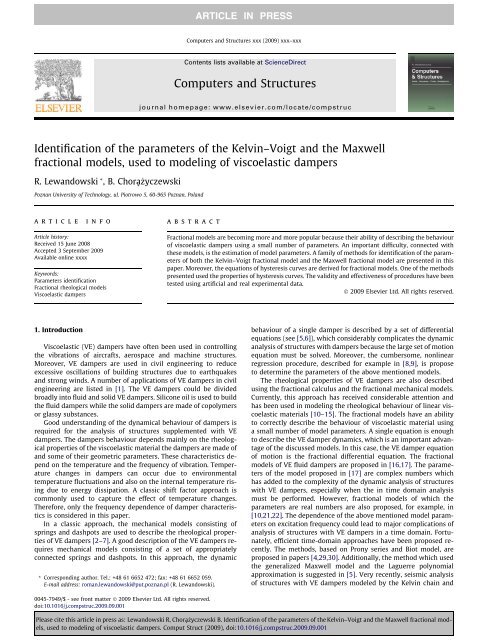
<strong>Identification</strong> <strong>of</strong> <strong>the</strong> <strong>parameters</strong> <strong>of</strong> <strong>the</strong> Kelvin–Voigt <strong>and</strong> <strong>the</strong> <strong>Maxwell</strong><br />
fractional models, used to modeling <strong>of</strong> viscoelastic dampers<br />
R. Lew<strong>and</strong>owski * , B. Chorą_zyczewski<br />
Poznan University <strong>of</strong> Technology, ul. Piotrowo 5, 60-965 Poznan, Pol<strong>and</strong><br />
article<br />
info<br />
abstract<br />
Article history:<br />
Received 15 June 2008<br />
Accepted 3 September 2009<br />
Available online xxxx<br />
Keywords:<br />
Parameters identification<br />
Fractional rheological models<br />
Viscoelastic dampers<br />
Fractional models are becoming more <strong>and</strong> more popular because <strong>the</strong>ir ability <strong>of</strong> describing <strong>the</strong> behaviour<br />
<strong>of</strong> viscoelastic dampers using a small number <strong>of</strong> <strong>parameters</strong>. An important difficulty, connected with<br />
<strong>the</strong>se models, is <strong>the</strong> estimation <strong>of</strong> model <strong>parameters</strong>. A family <strong>of</strong> methods for identification <strong>of</strong> <strong>the</strong> <strong>parameters</strong><br />
<strong>of</strong> both <strong>the</strong> Kelvin–Voigt fractional model <strong>and</strong> <strong>the</strong> <strong>Maxwell</strong> fractional model are presented in this<br />
paper. Moreover, <strong>the</strong> equations <strong>of</strong> hysteresis curves are derived for fractional models. One <strong>of</strong> <strong>the</strong> methods<br />
presented used <strong>the</strong> properties <strong>of</strong> hysteresis curves. The validity <strong>and</strong> effectiveness <strong>of</strong> procedures have been<br />
tested using artificial <strong>and</strong> real experimental data.<br />
Ó 2009 Elsevier Ltd. All rights reserved.<br />
1. Introduction<br />
Viscoelastic (VE) dampers have <strong>of</strong>ten been used in controlling<br />
<strong>the</strong> vibrations <strong>of</strong> aircrafts, aerospace <strong>and</strong> machine structures.<br />
Moreover, VE dampers are used in civil engineering to reduce<br />
excessive oscillations <strong>of</strong> building structures due to earthquakes<br />
<strong>and</strong> strong winds. A number <strong>of</strong> applications <strong>of</strong> VE dampers in civil<br />
engineering are listed in [1]. The VE dampers could be divided<br />
broadly into fluid <strong>and</strong> solid VE dampers. Silicone oil is used to build<br />
<strong>the</strong> fluid dampers while <strong>the</strong> solid dampers are made <strong>of</strong> copolymers<br />
or glassy substances.<br />
Good underst<strong>and</strong>ing <strong>of</strong> <strong>the</strong> dynamical behaviour <strong>of</strong> dampers is<br />
required for <strong>the</strong> analysis <strong>of</strong> structures supplemented with VE<br />
dampers. The dampers behaviour depends mainly on <strong>the</strong> rheological<br />
properties <strong>of</strong> <strong>the</strong> viscoelastic material <strong>the</strong> dampers are made <strong>of</strong><br />
<strong>and</strong> some <strong>of</strong> <strong>the</strong>ir geometric <strong>parameters</strong>. These characteristics depend<br />
on <strong>the</strong> temperature <strong>and</strong> <strong>the</strong> frequency <strong>of</strong> vibration. Temperature<br />
changes in dampers can occur due to environmental<br />
temperature fluctuations <strong>and</strong> also on <strong>the</strong> internal temperature rising<br />
due to energy dissipation. A classic shift factor approach is<br />
commonly used to capture <strong>the</strong> effect <strong>of</strong> temperature changes.<br />
Therefore, only <strong>the</strong> frequency dependence <strong>of</strong> damper characteristics<br />
is considered in this paper.<br />
In a classic approach, <strong>the</strong> mechanical models consisting <strong>of</strong><br />
springs <strong>and</strong> dashpots are used to describe <strong>the</strong> rheological properties<br />
<strong>of</strong> VE dampers [2–7]. A good description <strong>of</strong> <strong>the</strong> VE dampers requires<br />
mechanical models consisting <strong>of</strong> a set <strong>of</strong> appropriately<br />
connected springs <strong>and</strong> dashpots. In this approach, <strong>the</strong> dynamic<br />
* Corresponding author. Tel.: +48 61 6652 472; fax: +48 61 6652 059.<br />
E-mail address: roman.lew<strong>and</strong>owski@put.poznan.pl (R. Lew<strong>and</strong>owski).<br />
behaviour <strong>of</strong> a single damper is described by a set <strong>of</strong> differential<br />
equations (see [5,6]), which considerably complicates <strong>the</strong> dynamic<br />
analysis <strong>of</strong> structures with dampers because <strong>the</strong> large set <strong>of</strong> motion<br />
equation must be solved. Moreover, <strong>the</strong> cumbersome, nonlinear<br />
regression procedure, described for example in [8,9], is propose<br />
to determine <strong>the</strong> <strong>parameters</strong> <strong>of</strong> <strong>the</strong> above mentioned models.<br />
The rheological properties <strong>of</strong> VE dampers are also described<br />
using <strong>the</strong> fractional calculus <strong>and</strong> <strong>the</strong> fractional mechanical models.<br />
Currently, this approach has received considerable attention <strong>and</strong><br />
has been used in modeling <strong>the</strong> rheological behaviour <strong>of</strong> linear viscoelastic<br />
materials [10–15]. The fractional models have an ability<br />
to correctly describe <strong>the</strong> behaviour <strong>of</strong> viscoelastic material using<br />
a small number <strong>of</strong> model <strong>parameters</strong>. A single equation is enough<br />
to describe <strong>the</strong> VE damper dynamics, which is an important advantage<br />
<strong>of</strong> <strong>the</strong> discussed models. In this case, <strong>the</strong> VE damper equation<br />
<strong>of</strong> motion is <strong>the</strong> fractional differential equation. The fractional<br />
models <strong>of</strong> VE fluid dampers are proposed in [16,17]. The <strong>parameters</strong><br />
<strong>of</strong> <strong>the</strong> model proposed in [17] are complex numbers which<br />
has added to <strong>the</strong> complexity <strong>of</strong> <strong>the</strong> dynamic analysis <strong>of</strong> structures<br />
with VE dampers, especially when <strong>the</strong> in time domain analysis<br />
must be performed. However, fractional models <strong>of</strong> which <strong>the</strong><br />
<strong>parameters</strong> are real numbers are also proposed, for example, in<br />
[10,21,22]. The dependence <strong>of</strong> <strong>the</strong> above mentioned model <strong>parameters</strong><br />
on excitation frequency could lead to major complications <strong>of</strong><br />
analysis <strong>of</strong> structures with VE dampers in a time domain. Fortunately,<br />
efficient time-domain approaches have been proposed recently.<br />
The methods, based on Prony series <strong>and</strong> Biot model, are<br />
proposed in papers [4,29,30]. Additionally, <strong>the</strong> method which used<br />
<strong>the</strong> generalized <strong>Maxwell</strong> model <strong>and</strong> <strong>the</strong> Laguerre polynomial<br />
approximation is suggested in [5]. Very recently, seismic analysis<br />
<strong>of</strong> structures with VE dampers modeled by <strong>the</strong> Kelvin chain <strong>and</strong><br />
0045-7949/$ - see front matter Ó 2009 Elsevier Ltd. All rights reserved.<br />
doi:10.1016/j.compstruc.2009.09.001<br />
Please cite this article in press as: Lew<strong>and</strong>owski R, Chorą _zyczewski B. <strong>Identification</strong> <strong>of</strong> <strong>the</strong> <strong>parameters</strong> <strong>of</strong> <strong>the</strong> Kelvin–Voigt <strong>and</strong> <strong>the</strong> <strong>Maxwell</strong> fractional models,<br />
used to modeling <strong>of</strong> viscoelastic dampers. Comput Struct (2009), doi:10.1016/j.compstruc.2009.09.001
ARTICLE IN PRESS<br />
2 R. Lew<strong>and</strong>owski, B. Chorą_zyczewski / Computers <strong>and</strong> Structures xxx (2009) xxx–xxx<br />
<strong>the</strong> <strong>Maxwell</strong> ladder is presented in [6]. Moreover, <strong>the</strong> non-viscous<br />
state-space model, described in [31], could be used in this context.<br />
The analysis in <strong>the</strong> frequency domain is possible <strong>and</strong> presented, for<br />
example, in [3].<br />
An important problem, connected with <strong>the</strong> fractional rheological<br />
models, is an estimation <strong>of</strong> <strong>the</strong> model <strong>parameters</strong> from experimental<br />
data. In <strong>the</strong> past, different methods have been tested for<br />
<strong>the</strong> estimation <strong>of</strong> model <strong>parameters</strong> from both static <strong>and</strong> dynamic<br />
experiments [4,8,9,16–19,21]. The process <strong>of</strong> parameter identification<br />
is an inverse problem which is overdetermined <strong>and</strong> can be ill<br />
conditioned (see, for example [8,19]) because <strong>of</strong> noises existing in<br />
<strong>the</strong> experimental data. The ma<strong>the</strong>matical difficulties may be overcome<br />
by <strong>the</strong> regularization method which is described, for example,<br />
in [8,18].<br />
It is <strong>the</strong> aim <strong>of</strong> this paper to describe a few methods <strong>of</strong> identification<br />
<strong>of</strong> <strong>the</strong> <strong>parameters</strong> <strong>of</strong> VE dampers. The <strong>parameters</strong> are estimated<br />
using <strong>the</strong> results obtained from dynamical tests. The<br />
fractional rheological models are used to describe <strong>the</strong> dynamic<br />
behaviour <strong>of</strong> dampers. The Kelvin–Voigt model <strong>and</strong> <strong>the</strong> <strong>Maxwell</strong><br />
model are discussed. Three kinds <strong>of</strong> identification methods are suggested.<br />
Equations <strong>of</strong> hysteresis curves are derived for both fractional<br />
models <strong>and</strong> some <strong>of</strong> <strong>the</strong> properties <strong>of</strong> <strong>the</strong>se curves are<br />
used to develop <strong>the</strong> first-kind identification procedure. The second-<br />
<strong>and</strong> third-kind identification procedures are based on time<br />
series data. Each identification procedure consists <strong>of</strong> two main<br />
steps. In <strong>the</strong> first step, for <strong>the</strong> given frequencies <strong>of</strong> excitation,<br />
experimentally obtained data are approximated by simple harmonic<br />
functions while model <strong>parameters</strong> are determined in <strong>the</strong><br />
second stage <strong>of</strong> <strong>the</strong> identification procedure. The results <strong>of</strong> a typical<br />
calculation are presented <strong>and</strong> discussed.<br />
Three symbols will be used in <strong>the</strong> paper to describe <strong>the</strong> damper<br />
force. The symbol u e ðtÞ denotes <strong>the</strong> results <strong>of</strong> experimental measurements,<br />
~uðtÞ is <strong>the</strong> function which is an analytical approximation<br />
<strong>of</strong> experimental results while uðtÞ is <strong>the</strong> solution to <strong>the</strong><br />
damper equation <strong>of</strong> motion. The symbols q e ðtÞ; ~qðtÞ <strong>and</strong> qðtÞ are<br />
used in <strong>the</strong> same way to describe <strong>the</strong> damper displacement.<br />
2. General explanation <strong>of</strong> fractional rheological models<br />
Due to <strong>the</strong>ir simplicity, <strong>the</strong> simple rheological models, such as<br />
<strong>the</strong> Kelvin–Voigt model or <strong>the</strong> <strong>Maxwell</strong> model, are used very <strong>of</strong>ten<br />
to describe <strong>the</strong> dynamic behavior <strong>of</strong> VE dampers installed on<br />
various types <strong>of</strong> civil structures. For example, <strong>the</strong> Kelvin–Voigt<br />
model is used in papers [2,3,22–24], while <strong>the</strong> <strong>Maxwell</strong> model<br />
is used in papers [2,3,25–28]. The Kelvin–Voigt model consists<br />
<strong>of</strong> <strong>the</strong> spring <strong>and</strong> <strong>the</strong> dashpot connected in parallel, while <strong>the</strong><br />
<strong>Maxwell</strong> model is built from <strong>the</strong> serially connected spring <strong>and</strong><br />
dashpot. The discussed simple rheological models have a small<br />
number <strong>of</strong> <strong>parameters</strong> but do not have enough <strong>parameters</strong> to<br />
accurately capture <strong>the</strong> frequency dependence <strong>of</strong> damper <strong>parameters</strong>.<br />
More sophisticated classical rheological models which, however,<br />
contain many <strong>parameters</strong>, can be used to correctly describe<br />
<strong>the</strong> dynamic behavior <strong>of</strong> VE dampers. Models <strong>of</strong> this kind are<br />
developed in [6,7].<br />
The next group <strong>of</strong> models used to describe <strong>the</strong> behaviour <strong>of</strong> VE<br />
dampers are <strong>the</strong> fractional derivative models. Using <strong>the</strong> fractional<br />
calculus, a number <strong>of</strong> rheological models, e.g., <strong>the</strong> fractional Kelvin–Voigt<br />
model [32], <strong>the</strong> fractional Zener model [10,11], <strong>the</strong> fractional<br />
Jeffreys model [12], or <strong>the</strong> fractional <strong>Maxwell</strong> model [17] can<br />
be developed. It has been proved in [4,15] that <strong>the</strong> fractional derivative<br />
models can better capture <strong>the</strong> frequency dependent properties<br />
<strong>of</strong> VE dampers. The simple fractional models discussed in<br />
[4,13,15] are sufficient to correctly capture <strong>the</strong> VE dampers properties.<br />
These models contain only a few <strong>parameters</strong> but <strong>the</strong> dynamic<br />
analysis requires knowledge <strong>of</strong> <strong>the</strong> fractional calculus.<br />
The simple Kelvin–Voigt model seems to be more appropriate<br />
to describe <strong>the</strong> solid dampers behavior, while <strong>the</strong> simple <strong>Maxwell</strong><br />
model is mainly used to describe <strong>the</strong> liquid dampers behavior. Recently,<br />
it has been shown in [6] that both <strong>the</strong> generalized Kelvin<br />
model <strong>and</strong> <strong>the</strong> generalized <strong>Maxwell</strong> model are also useful models<br />
<strong>of</strong> <strong>the</strong> solid VE damper.<br />
One important problem, considered here <strong>and</strong> connected with<br />
<strong>the</strong>se models, is how to determine model <strong>parameters</strong> from experimental<br />
data in an efficient way. This problem is solved in this Section<br />
for <strong>the</strong> fractional Kelvin–Voigt model <strong>and</strong> <strong>the</strong> fractional<br />
<strong>Maxwell</strong> model.<br />
2.1. Fractional models equation <strong>of</strong> motion <strong>and</strong> <strong>the</strong> steady state solution<br />
to <strong>the</strong> motion equation<br />
In order to construct <strong>the</strong> fractional models equation <strong>of</strong> motion,<br />
we introduce <strong>the</strong> fractional element called <strong>the</strong> springpot which<br />
satisfies <strong>the</strong> constitutive equation:<br />
uðtÞ ¼~c a D a t qðtÞ ¼cDa t qðtÞ;<br />
where c ¼ ~c a <strong>and</strong> a; 0 < a 6 1, are <strong>the</strong> springpot <strong>parameters</strong> <strong>and</strong><br />
D a t<br />
qðtÞ is <strong>the</strong> fractional derivative <strong>of</strong> <strong>the</strong> order a with respect to time<br />
t. There are a few definitions <strong>of</strong> fractional derivatives which coincide<br />
under certain conditions. Here, symbols such as D a t<br />
qðtÞ denote<br />
<strong>the</strong> Riemann–Liouville fractional derivatives with <strong>the</strong> lower limit at<br />
– 1 (see [34]). Some valuable information about fractional calculus<br />
can be found in [34].<br />
The springpot element, also known as <strong>the</strong> Scott–Blair’s element<br />
(see [33]), is schematically shown in Fig. 1a. The considered element<br />
can be understood as an interpolation between <strong>the</strong> spring<br />
element ða ¼ 0Þ <strong>and</strong> <strong>the</strong> dashpot element ða ¼ 1Þ.<br />
The fractional Kelvin–Voigt model consists <strong>of</strong> <strong>the</strong> spring<br />
<strong>and</strong> <strong>the</strong> springpot connected in parallel, while <strong>the</strong> fractional<br />
<strong>Maxwell</strong> model is built <strong>of</strong> <strong>the</strong> serially connected spring <strong>and</strong> springpot.<br />
These models are shown schematically in Fig. 1b <strong>and</strong> c,<br />
respectively.<br />
The motion equation <strong>of</strong> <strong>the</strong> above mentioned fractional Kelvin–<br />
Voigt model, obtained in a usual way, is in <strong>the</strong> following form:<br />
uðtÞ ¼kqðtÞþks a D a t qðtÞ;<br />
where s a ¼ ~c a =k ¼ c=k.<br />
The following relationships can be written for <strong>the</strong> fractional<br />
<strong>Maxwell</strong> model (Fig. 1c)<br />
uðtÞ ¼kq 1 ðtÞ; uðtÞ ¼~c a D a t ðqðtÞ q 1ðtÞÞ: ð3Þ<br />
Eliminating q 1 ðtÞ from <strong>the</strong> above relationships, we get <strong>the</strong> equation<br />
in <strong>the</strong> form:<br />
uðtÞþs a D a t uðtÞ ¼ksa D a t qðtÞ:<br />
ð4Þ<br />
It is easy to recognize that both <strong>of</strong> <strong>the</strong> considered fractional models<br />
have three real <strong>and</strong> positive value <strong>parameters</strong>: k, c, <strong>and</strong> a.<br />
In <strong>the</strong> case <strong>of</strong> a harmonically excited damper, i.e. when<br />
qðtÞ ¼q 0 expðiktÞ;<br />
<strong>the</strong> steady state solution <strong>of</strong> <strong>the</strong> motion equation <strong>of</strong> both <strong>of</strong> <strong>the</strong> fractional<br />
models is assumed in <strong>the</strong> form:<br />
uðtÞ ¼u 0 expðiktÞ:<br />
Taking into account that in our case (see [34, p. 311])<br />
D a t expðiktÞ ¼ðikÞa expðiktÞ;<br />
for k > 0, we obtain <strong>the</strong> following equations<br />
u 0 ¼ k½1 þðiskÞ a ðiskÞ a<br />
Šq 0 ; u 0 ¼ k<br />
1 þðiskÞ a q 0 ; ð8Þ<br />
ð1Þ<br />
ð2Þ<br />
ð5Þ<br />
ð6Þ<br />
ð7Þ<br />
Please cite this article in press as: Lew<strong>and</strong>owski R, Chorą _zyczewski B. <strong>Identification</strong> <strong>of</strong> <strong>the</strong> <strong>parameters</strong> <strong>of</strong> <strong>the</strong> Kelvin–Voigt <strong>and</strong> <strong>the</strong> <strong>Maxwell</strong> fractional models,<br />
used to modeling <strong>of</strong> viscoelastic dampers. Comput Struct (2009), doi:10.1016/j.compstruc.2009.09.001
ARTICLE IN PRESS<br />
R. Lew<strong>and</strong>owski, B. Chorą_zyczewski / Computers <strong>and</strong> Structures xxx (2009) xxx–xxx 3<br />
Fig. 1. Diagram <strong>of</strong> fractional rheological models.<br />
from (2) <strong>and</strong> (4), respectively. Moreover, after introducing <strong>the</strong> following<br />
formula i a ¼ cosðap=2Þþi sinðap=2Þ, we can rewrite relationships<br />
(8) in <strong>the</strong> form<br />
u 0 ¼ðK 0 þ iK 00 Þq 0 ¼ K 0 ð1 þ igÞq 0 ;<br />
where gðkÞ ¼K 00 ðkÞ=K 0 ðkÞ is <strong>the</strong> loss factor, K 0 ðkÞ is <strong>the</strong> storage<br />
modulus <strong>and</strong> K 00 ðkÞ is <strong>the</strong> loss modulus. These quantities are defined<br />
as:<br />
K 0 ¼ k½1 þðskÞ a cosðap=2ÞŠ; K 00 ¼ kðskÞ a sinðap=2Þ; ð10Þ<br />
g ¼<br />
ðskÞa sinðap=2Þ<br />
1 þðskÞ a cosðap=2Þ ; ð11Þ<br />
for <strong>the</strong> fractional Kelvin–Voigt model <strong>and</strong><br />
K 0 ¼ kðskÞ a ðskÞ a þ cosðap=2Þ<br />
1 þðskÞ 2a þ 2ðskÞ a cosðap=2Þ ;<br />
K 00 ¼ kðskÞ a sinðap=2Þ<br />
1 þðskÞ 2a þ 2ðskÞ a cosðap=2Þ ; ð12Þ<br />
sinðap=2Þ<br />
g ¼<br />
ðskÞ a þ cosðap=2Þ ;<br />
ð13Þ<br />
for <strong>the</strong> fractional <strong>Maxwell</strong> model.<br />
If <strong>the</strong> classical Kelvin–Voigt model (i.e. a ¼ 1Þ is used as <strong>the</strong> VE<br />
dampers model <strong>the</strong> above mentioned quantities are given by<br />
K 0 ðkÞ ¼k; K 00 ðkÞ ¼ksk; gðkÞ ¼K 00 ðkÞ=K 0 ðkÞ ¼sk ð14Þ<br />
while for <strong>the</strong> classical <strong>Maxwell</strong> model we have<br />
s<br />
K 0 2 k 2<br />
ðkÞ ¼k<br />
1 þ s 2 k ; sk<br />
2 K00 ðkÞ ¼k<br />
1 þ s 2 k ; gðkÞ ¼ 1 2 sk : ð15Þ<br />
The dependence <strong>of</strong> <strong>the</strong> above mentioned model <strong>parameters</strong> on excitation<br />
frequency could significantly complicates in time domain<br />
analysis <strong>of</strong> structures with VE dampers.<br />
According to <strong>the</strong> classical Kelvin–Voigt model <strong>the</strong> storage modulus<br />
is <strong>the</strong> constant function <strong>of</strong> k, while <strong>the</strong> loss modulus <strong>and</strong> <strong>the</strong><br />
loss factor linearly increases with k. Behaviour <strong>of</strong> <strong>the</strong> fractional Kelvin–Voigt<br />
model is substantially different in comparison with <strong>the</strong><br />
classic Kelvin–Voigt model. The storage modulus is increased significantly<br />
when <strong>the</strong> non-dimensional frequency increases <strong>and</strong><br />
when <strong>the</strong> parameter a decreases. Moreover, <strong>the</strong> loss modulus<br />
<strong>and</strong> <strong>the</strong> loss factor decrease for an increasing non-dimensional frequency<br />
<strong>and</strong> <strong>the</strong> decreasing values <strong>of</strong> <strong>the</strong> parameter a.<br />
The properties <strong>of</strong> <strong>the</strong> fractional <strong>Maxwell</strong> model, for different<br />
values <strong>of</strong> <strong>the</strong> parameter a are shown in Figs. 2 <strong>and</strong> 3. In <strong>the</strong> figures<br />
<strong>the</strong> non-dimensional frequency is defined as sk. The calculation is<br />
made using <strong>the</strong> value <strong>of</strong> <strong>the</strong> k parameter equal to 1,00,000.0 N/m.<br />
ð9Þ<br />
The storage modulus grows with non-dimensional frequency for<br />
all values <strong>of</strong> <strong>the</strong> parameter a. However, for 0 < sk < 1 <strong>the</strong> function<br />
K 0 ðaÞ increases for decreasing values <strong>of</strong> a. An opposite tendency is<br />
evident for sk > 1. The function <strong>of</strong> <strong>the</strong> loss modulus could be flat<br />
(for instant when a ¼ 0:4Þ. Moreover, gð0Þ ¼tgðap=2Þ which<br />
means that <strong>the</strong> loss factor has a finite value for k ¼ 0. This is an<br />
important difference in comparison with <strong>the</strong> loss factor function<br />
<strong>of</strong> <strong>the</strong> classic <strong>Maxwell</strong> model <strong>of</strong> which <strong>the</strong> values approach infinity<br />
if k approaches zero <strong>and</strong> in comparison with <strong>the</strong> both versions <strong>of</strong><br />
<strong>the</strong> Kelvin–Voigt model for which <strong>the</strong> loss factor is equal to zero<br />
for sk ¼ 0.<br />
According to results presented by Lion in [35] <strong>the</strong> fractional rheological<br />
models fulfill <strong>the</strong> second law <strong>of</strong> <strong>the</strong>rmodynamics when<br />
values <strong>of</strong> <strong>the</strong> storage modulus K 0 ðkÞ <strong>and</strong> <strong>the</strong> loss modulus K 00 ðkÞ, given<br />
by formulae (10)–(13), are positive for all possible values <strong>of</strong><br />
frequency <strong>of</strong> excitation k. It can easily be demonstrated that both<br />
models fulfill <strong>the</strong> second law <strong>of</strong> <strong>the</strong>rmodynamics when<br />
0 6 a 6 1; s > 0 <strong>and</strong> k > 0.<br />
If <strong>the</strong> damper displacement varies harmonically in time <strong>and</strong> is<br />
described using <strong>the</strong> trigonometric functions, i.e.:<br />
qðtÞ ¼q c cos kt þ q s sin kt;<br />
ð16Þ<br />
<strong>the</strong> steady state solution to <strong>the</strong> fractional Kelvin–Voigt model equation<br />
<strong>of</strong> motion (2) is given by<br />
uðtÞ ¼u c cos kt þ u s sin kt;<br />
where<br />
ð17Þ<br />
u c ¼ u 1<br />
q c þ u 2<br />
q s ; u s ¼ u 2<br />
q c þ u 1<br />
q s ; ð18Þ<br />
u 1<br />
¼ k þ ck a cosðap=2Þ; u 2<br />
¼ ck a sinðap=2Þ: ð19Þ<br />
The steady state solution to <strong>the</strong> equation <strong>of</strong> motion (4) <strong>of</strong> <strong>the</strong> fractional<br />
<strong>Maxwell</strong> model is also given by (16) <strong>and</strong> (17) <strong>and</strong> <strong>the</strong> coefficients<br />
q c ; q s ; u c <strong>and</strong> u s are interrelated in <strong>the</strong> following way:<br />
q c ¼ / 1 u c / 2 u s ; q s ¼ / 2 u c þ / 1 u s ; ð20Þ<br />
where<br />
h<br />
/ 1 ¼ 1<br />
kðskÞ a ðskÞ a þ cos ap 2<br />
i<br />
; / 2 ¼ 1<br />
kðskÞ a sin ap 2 :<br />
2.2. Hysteresis loops <strong>of</strong> <strong>the</strong> damper models<br />
ð21Þ<br />
The equation <strong>of</strong> <strong>the</strong> hysteresis loops <strong>of</strong> <strong>the</strong> fractional Kelvin–<br />
Voigt model could be derived if <strong>the</strong> damper’s kinematical excitation<br />
is given by<br />
qðtÞ ¼q 0 sin kt:<br />
ð22Þ<br />
Please cite this article in press as: Lew<strong>and</strong>owski R, Chorą _zyczewski B. <strong>Identification</strong> <strong>of</strong> <strong>the</strong> <strong>parameters</strong> <strong>of</strong> <strong>the</strong> Kelvin–Voigt <strong>and</strong> <strong>the</strong> <strong>Maxwell</strong> fractional models,<br />
used to modeling <strong>of</strong> viscoelastic dampers. Comput Struct (2009), doi:10.1016/j.compstruc.2009.09.001
ARTICLE IN PRESS<br />
4 R. Lew<strong>and</strong>owski, B. Chorą_zyczewski / Computers <strong>and</strong> Structures xxx (2009) xxx–xxx<br />
Fig. 2. The storage modulus <strong>of</strong> <strong>the</strong> fractional <strong>Maxwell</strong> model for different values <strong>of</strong> a parameter.<br />
Fig. 3. The loss modulus <strong>of</strong> <strong>the</strong> fractional <strong>Maxwell</strong> model for different values <strong>of</strong> a parameter.<br />
Taking into account that (see [34, p. 311])<br />
D a t qðtÞ ¼ka q 0 sin½kt þðap=2ÞŠ;<br />
<strong>and</strong> introducing (22) <strong>and</strong> (23) into Eq. (2) we can write<br />
uðtÞ ¼k½1 þðskÞ a cosðap=2ÞŠq 0 sin kt þ kðskÞ a q 0 sinðap=2Þ cos kt:<br />
ð23Þ<br />
ð24Þ<br />
Next, using (22) <strong>and</strong> <strong>the</strong> identity sin 2 ðap=2Þþcos 2 ðap=2Þ ¼1, we<br />
can rewrite (24) in <strong>the</strong> form <strong>of</strong> <strong>the</strong> following equation<br />
<br />
uðtÞ k½1 þðskÞ a 2 <br />
cosðap=2ÞŠqðtÞ<br />
kðskÞ a þ qðtÞ 2<br />
¼ 1; ð25Þ<br />
q 0 sinðap=2Þ<br />
which describes <strong>the</strong> first version <strong>of</strong> <strong>the</strong> hysteresis loop <strong>of</strong> <strong>the</strong> fractional<br />
Kelvin–Voigt model.<br />
Derivation <strong>of</strong> <strong>the</strong> second version <strong>of</strong> <strong>the</strong> hysteresis loop started<br />
with an assumption that <strong>the</strong> damper’s displacement is described<br />
by<br />
qðtÞ ¼q 0 sin½kt ðap=2ÞŠ; ð26Þ<br />
q 0<br />
which means that<br />
D a t qðtÞ ¼ka q 0 sin kt:<br />
ð27Þ<br />
Introducing relationship (26) into <strong>the</strong> motion Eq. (2) we can write<br />
uðtÞ ks a D a t qðtÞ ¼kq 0½sin kt cosðap=2Þ cos kt sinðap=2ÞŠ: ð28Þ<br />
Using (27) it is possible to write <strong>the</strong> second version <strong>of</strong> <strong>the</strong> hysteresis<br />
loop equation in <strong>the</strong> following form:<br />
<br />
uðtÞ<br />
kk a ½ðskÞ a þ cosðap=2ÞŠD a t qðtÞ<br />
kq 0 sinðap=2Þ<br />
2 <br />
þ Da t qðtÞ 2<br />
k a ¼ 1: ð29Þ<br />
q 0<br />
In a case <strong>of</strong> <strong>the</strong> classical Kelvin–Voigt model we have:<br />
<br />
2 <br />
uðtÞ kqðtÞ<br />
þ qðtÞ 2 2 <br />
uðtÞ c _qðtÞ<br />
¼ 1;<br />
þ _ 2<br />
qðtÞ<br />
kcq 0 q 0<br />
kq 0 kq 0<br />
¼ 1;<br />
instead <strong>of</strong> (25) <strong>and</strong> (29).<br />
ð30Þ<br />
Please cite this article in press as: Lew<strong>and</strong>owski R, Chorą _zyczewski B. <strong>Identification</strong> <strong>of</strong> <strong>the</strong> <strong>parameters</strong> <strong>of</strong> <strong>the</strong> Kelvin–Voigt <strong>and</strong> <strong>the</strong> <strong>Maxwell</strong> fractional models,<br />
used to modeling <strong>of</strong> viscoelastic dampers. Comput Struct (2009), doi:10.1016/j.compstruc.2009.09.001
ARTICLE IN PRESS<br />
R. Lew<strong>and</strong>owski, B. Chorą_zyczewski / Computers <strong>and</strong> Structures xxx (2009) xxx–xxx 5<br />
Let us now proceed to developing <strong>the</strong> equation describing <strong>the</strong><br />
hysteresis loop <strong>of</strong> <strong>the</strong> fractional <strong>Maxwell</strong> model. The excitation is<br />
described by<br />
uðtÞ ¼u 0 sin kt;<br />
what means that<br />
D a t uðtÞ ¼ka u 0 sin½kt þðap=2ÞŠ:<br />
ð31Þ<br />
ð32Þ<br />
Introducing (32) into <strong>the</strong> motion Eq. (4) we obtain <strong>the</strong> following<br />
relationship<br />
uðtÞ ks a D a t qðtÞ ¼ ðskÞa u 0 ½sin kt cosðap=2Þþcos kt sinðap=2ÞŠ;<br />
ð33Þ<br />
which could be rewritten as<br />
<br />
ks a D a t qðtÞ ½1 2 þðskÞa cosðap=2ÞŠuðtÞ<br />
ðskÞ a þ uðtÞ 2<br />
¼ 1: ð34Þ<br />
u 0 sinðap=2Þ<br />
This is <strong>the</strong> first version <strong>of</strong> <strong>the</strong> hysteresis loop equation <strong>of</strong> <strong>the</strong> fractional<br />
<strong>Maxwell</strong> model.<br />
To obtain <strong>the</strong> second version <strong>of</strong> <strong>the</strong> hysteresis loop equation <strong>the</strong><br />
motion Eq. (4) must be fractionally integrated. This operation is<br />
formally defined in [34] <strong>and</strong> here it will be denoted using <strong>the</strong> symbol<br />
D a<br />
t<br />
uðtÞ if <strong>the</strong> function uðtÞ is integrated. Moreover, it can be<br />
demonstrated that D a<br />
t<br />
ðD a t<br />
uðtÞÞ ¼ uðtÞ.<br />
After <strong>the</strong> fractional integration <strong>of</strong> Eq. (4) we obtain<br />
D a<br />
t<br />
uðtÞþs a uðtÞ ¼ks a qðtÞ: ð35Þ<br />
Now, if uðtÞ is given by (31) <strong>the</strong>n<br />
D a<br />
t<br />
ðu 0 sin ktÞ ¼u 0 k a sin½kt ðap=2ÞŠ: ð36Þ<br />
Introducing (31) into (4) we can write Eq. (35) in <strong>the</strong> form:<br />
u 0<br />
kðskÞ a qðtÞ<br />
ðskÞ a uðtÞ ¼u 0 ½sin kt cosðap=2Þ<br />
cos kt sinðap=2ÞŠ:<br />
ð37Þ<br />
Next, with <strong>the</strong> help <strong>of</strong> relationships (31) <strong>and</strong> sin 2 ðap=2Þþ<br />
cos 2 ðap=2Þ ¼1 we can transform <strong>the</strong> above equation to<br />
<br />
kðskÞ a qðtÞ<br />
½ðskÞ a þ cosðap=2ÞŠuðtÞ<br />
u 0 sinðap=2Þ<br />
2 <br />
þ uðtÞ 2<br />
¼ 1; ð38Þ<br />
which is <strong>the</strong> second version <strong>of</strong> <strong>the</strong> hysteresis loop equation<br />
searched for.<br />
It is obvious that, for <strong>the</strong> classical <strong>Maxwell</strong> model ða ¼ 1Þ we<br />
obtain:<br />
<br />
2 <br />
c _qðtÞ uðtÞ<br />
þ uðtÞ 2 <br />
2 <br />
¼ 1; ðskÞ 2 kqðtÞ uðtÞ<br />
þ uðtÞ 2<br />
¼ 1;<br />
sku 0 u 0<br />
u 0<br />
u 0<br />
ð39Þ<br />
instead <strong>of</strong> (34) <strong>and</strong> (38), respectively.<br />
The hysteresis loops <strong>of</strong> <strong>the</strong> fractional Kelvin–Voigt model <strong>and</strong><br />
<strong>the</strong> fractional <strong>Maxwell</strong> model are shown in Figs. 4 <strong>and</strong> 5, respectively,<br />
for different values <strong>of</strong> a <strong>and</strong> for k = 1,00,000.0 N/m, c =<br />
1,00,000.0 Ns/m, k = 10.0 rad/s. It is evident that for both models<br />
<strong>the</strong> damper’s damping abilities decrease as <strong>the</strong> values <strong>of</strong> a<br />
decrease.<br />
3. General remarks concerning identification methods<br />
The problem <strong>of</strong> determination <strong>of</strong> <strong>the</strong> <strong>parameters</strong> <strong>of</strong> <strong>the</strong> fractional<br />
derivative rheological models is, more or less extensively,<br />
discussed in papers [10,13,17,20,21,37–40]. In two papers<br />
[10,13], Pritz describes <strong>the</strong> method <strong>of</strong> <strong>parameters</strong> identification<br />
<strong>of</strong> two fractional derivative rheological models with four <strong>and</strong> five<br />
<strong>parameters</strong>, respectively. The method utilizes some asymptotic<br />
properties <strong>of</strong> <strong>the</strong> storage <strong>and</strong> loss modulus functions, experimen-<br />
u 0<br />
Fig. 4. Hysteresis loops <strong>of</strong> <strong>the</strong> fractional Kelvin–Voigt model for different values <strong>of</strong> a.<br />
Please cite this article in press as: Lew<strong>and</strong>owski R, Chorą _zyczewski B. <strong>Identification</strong> <strong>of</strong> <strong>the</strong> <strong>parameters</strong> <strong>of</strong> <strong>the</strong> Kelvin–Voigt <strong>and</strong> <strong>the</strong> <strong>Maxwell</strong> fractional models,<br />
used to modeling <strong>of</strong> viscoelastic dampers. Comput Struct (2009), doi:10.1016/j.compstruc.2009.09.001
ARTICLE IN PRESS<br />
6 R. Lew<strong>and</strong>owski, B. Chorą_zyczewski / Computers <strong>and</strong> Structures xxx (2009) xxx–xxx<br />
Fig. 5. Hysteresis loops <strong>of</strong> <strong>the</strong> fractional <strong>Maxwell</strong> model for different values <strong>of</strong> a.<br />
tally obtained over a certain range <strong>of</strong> excitation frequencies. However,<br />
no systematic procedure <strong>of</strong> identification is presented. Similar<br />
methods are developed in [20,38] where more detailed<br />
description <strong>of</strong> identification procedure is also presented. The above<br />
mentioned methods require experimental data from a large range<br />
<strong>of</strong> excitation frequencies. Very recently, in paper [39], <strong>the</strong> identification<br />
procedure <strong>of</strong> <strong>parameters</strong> <strong>of</strong> fractional derivative model <strong>of</strong><br />
viscoelastic materials is also presented. The method uses an optimization<br />
procedure toge<strong>the</strong>r with <strong>the</strong> experimentally <strong>and</strong> numerically<br />
obtained frequency response functions to determine <strong>the</strong><br />
<strong>parameters</strong> <strong>of</strong> <strong>the</strong> considered model VE materials. The differences<br />
between <strong>the</strong> measured <strong>and</strong> calculated frequency response functions<br />
are minimized in order to estimate <strong>the</strong> true values <strong>of</strong> <strong>the</strong><br />
searched <strong>parameters</strong>. Moreover, <strong>the</strong> least squares method, in<br />
which <strong>the</strong> error between <strong>the</strong> model <strong>and</strong> <strong>the</strong> experimental complex<br />
modulus K ðkÞ; ðK ðkÞ ¼K 0 ðkÞþiK 00 ðkÞÞ is minimized in order to obtain<br />
<strong>the</strong> <strong>parameters</strong> <strong>of</strong> <strong>the</strong> fractional model <strong>of</strong> viscoelastic materials<br />
is suggested in [21,37,40]. Unfortunately, details <strong>of</strong> <strong>the</strong> used<br />
least squares method are presented in [40] only.<br />
There are many papers containing a description <strong>of</strong> <strong>the</strong> method<br />
<strong>of</strong> identification <strong>of</strong> <strong>parameters</strong> <strong>of</strong> <strong>the</strong> classic rheological models<br />
<strong>of</strong> VE materials <strong>and</strong> VE dampers. In paper [4] Park used <strong>the</strong> Prony<br />
series toge<strong>the</strong>r with <strong>the</strong> least squares method to determine <strong>parameters</strong><br />
<strong>of</strong> <strong>the</strong> generalized <strong>Maxwell</strong> model <strong>of</strong> <strong>the</strong> VE solid <strong>and</strong> <strong>the</strong> VE<br />
liquid damper. The normalized error between <strong>the</strong> experimentally<br />
obtained <strong>and</strong> <strong>the</strong> calculated complex modulus is minimized. The<br />
optimization problem is linear because <strong>the</strong> number <strong>of</strong> Prony series<br />
<strong>and</strong> <strong>the</strong> relaxation times are fixed. The last square method is also<br />
used in [6] to determine <strong>the</strong> <strong>parameters</strong> <strong>of</strong> two mechanical models<br />
<strong>of</strong> VE dampers. The models are <strong>the</strong> Kelvin chain <strong>and</strong> <strong>the</strong> <strong>Maxwell</strong><br />
ladder. Some information concerning identification <strong>of</strong> <strong>the</strong> <strong>parameters</strong><br />
<strong>of</strong> <strong>the</strong> so-called GHM model <strong>and</strong> <strong>the</strong> ADF model used for modeling<br />
viscoelastic materials are presented in [41]. The advanced<br />
numerical methods for parameter identification <strong>of</strong> VE materials<br />
are presented in [8,9,42] where <strong>the</strong> least squares method toge<strong>the</strong>r<br />
with <strong>the</strong> regularization technique is used to solve <strong>the</strong> considered<br />
identification problem.<br />
In this paper, <strong>the</strong> <strong>parameters</strong> <strong>of</strong> <strong>the</strong> fractional Kelvin model <strong>and</strong><br />
<strong>the</strong> fractional <strong>Maxwell</strong> model are determined using results <strong>of</strong> dynamic<br />
tests. The proposed identification methods differ substantially<br />
in comparison with <strong>the</strong> previously mentioned ones. First <strong>of</strong><br />
all, instead <strong>of</strong> using <strong>the</strong> experimentally obtained complex modulus<br />
<strong>the</strong> suggested methods utilize <strong>the</strong> measured steady state responses<br />
<strong>of</strong> damper. The previous methods, presented in [10,13,20,38], require<br />
experimental data from a large range <strong>of</strong> excitation frequency<br />
while <strong>the</strong> suggested methods could be also used when data are<br />
available only from a narrow range <strong>of</strong> excitation frequency. Moreover,<br />
<strong>the</strong> error functional minimized in <strong>the</strong> least squares method<br />
<strong>and</strong> adopted in our identification methods is different from one<br />
used in previous papers. The results <strong>of</strong> calculation show that <strong>the</strong><br />
proposed methods are not sensitive to measurements noises <strong>and</strong>,<br />
<strong>the</strong>refore, it is not necessary to use regularization techniques.<br />
Additionally, a detailed description <strong>of</strong> <strong>the</strong> proposed identification<br />
method <strong>and</strong> <strong>the</strong> identification procedure are presented.<br />
Three kinds <strong>of</strong> identification methods are suggested in this paper<br />
to determine three <strong>parameters</strong> <strong>of</strong> <strong>the</strong> fractional Kelvin–Voigt<br />
model <strong>and</strong> <strong>the</strong> fractional <strong>Maxwell</strong> model. Each identification procedure<br />
consists <strong>of</strong> two main steps. In <strong>the</strong> first step, for <strong>the</strong> given<br />
frequencies <strong>of</strong> excitation, experimentally obtained data are<br />
approximated by simple harmonic functions while model <strong>parameters</strong><br />
are determined in <strong>the</strong> second stage <strong>of</strong> <strong>the</strong> identification<br />
procedure.<br />
4. <strong>Identification</strong> <strong>of</strong> model <strong>parameters</strong> for fractional Kelvin–<br />
Voigt model<br />
4.1. <strong>Identification</strong> procedures based on hysteresis loop (first method)<br />
First <strong>of</strong> all, <strong>the</strong> first kind method based on <strong>the</strong> hysteresis loop<br />
<strong>and</strong> applied to <strong>the</strong> fractional Kelvin–Voigt model will be described.<br />
Please cite this article in press as: Lew<strong>and</strong>owski R, Chorą _zyczewski B. <strong>Identification</strong> <strong>of</strong> <strong>the</strong> <strong>parameters</strong> <strong>of</strong> <strong>the</strong> Kelvin–Voigt <strong>and</strong> <strong>the</strong> <strong>Maxwell</strong> fractional models,<br />
used to modeling <strong>of</strong> viscoelastic dampers. Comput Struct (2009), doi:10.1016/j.compstruc.2009.09.001
ARTICLE IN PRESS<br />
R. Lew<strong>and</strong>owski, B. Chorą_zyczewski / Computers <strong>and</strong> Structures xxx (2009) xxx–xxx 7<br />
Eq. (25) seems to be more useful in comparison with (29). If, for <strong>the</strong><br />
given frequency <strong>of</strong> excitation <strong>and</strong> t ¼ t 1 , we have qðt 1 Þ¼q 0 > 0<br />
<strong>and</strong> uðt 1 Þ¼u 1 > 0 <strong>the</strong>n from Eq. (25) it follows<br />
k½1 þðskÞ a cosðap=2ÞŠ ¼ k þ ck a cosðap=2Þ ¼u 1 =q 0 :<br />
ð40Þ<br />
Moreover, for t ¼ t 2 when qðt 2 Þ¼0 <strong>and</strong> uðt 2 Þ¼u 2 > 0 from (25) we<br />
obtain<br />
kðskÞ a sinðap=2Þ ¼ck a sinðap=2Þ ¼u 2 =q 0 :<br />
ð41Þ<br />
For a given frequency k, relationships (40) <strong>and</strong> (41) constitute a set<br />
<strong>of</strong> two nonlinear equations with three unknowns: k; c; a or k; s; a.<br />
The quantities u 1 ; u 2 <strong>and</strong> q 0 have clear physical meanings <strong>and</strong> <strong>the</strong>ir<br />
values can easily be obtained from <strong>the</strong> experimental data. Alternatively,<br />
<strong>the</strong>se quantities could be calculated from trigonometric functions<br />
(A1) <strong>and</strong> (A6) used for <strong>the</strong> approximation <strong>of</strong> experimental<br />
data. Details are given in Appendix A. For a given a, <strong>the</strong> above set<br />
<strong>of</strong> equations are linear with respect to k <strong>and</strong> c.<br />
During experiments <strong>the</strong> damper is several times harmonically<br />
excited <strong>and</strong> in each case <strong>the</strong> excitation frequency, denoted here<br />
as k i , ði ¼ 1; 2; ::; nÞ, is different. The steady state response <strong>of</strong> <strong>the</strong><br />
damper is measured, which means that <strong>the</strong> experimental damper<br />
displacements q ei ðtÞ <strong>and</strong> <strong>the</strong> experimental damper forces u ei ðtÞ<br />
<strong>and</strong> functions ~q i ðtÞ ~u i ðtÞ which approximate <strong>the</strong> experimental data<br />
are known for each excitation frequency k i . Moreover, <strong>the</strong> above<br />
mentioned quantities, such as u 1 ; u 2 <strong>and</strong> q 0 can easily be determined<br />
for each excitation frequency. These quantities obtained<br />
from experimental data are denoted as u 1i ; u 2i <strong>and</strong> q 0i .<br />
Now it is assumed that resulting quantities u 1i ; u 2i <strong>and</strong> q 0i<br />
approximately fulfill relationships (40) <strong>and</strong> (41). For each excitation<br />
frequency we can write<br />
r i ¼ k þ ck a i<br />
cosðap=2Þ u 1i =q 0i 0; ð42Þ<br />
s i ¼ ck a i<br />
sinðap=2Þ u 2i =q 0i 0; ð43Þ<br />
where i ¼ 1; 2; ::; n. Symbols r i <strong>and</strong> s i denote residuals obtained after<br />
introducing u 1i ; u 2i <strong>and</strong> q 0i into (42) <strong>and</strong> (43).<br />
The above equations constitute a set <strong>of</strong> overdetermined nonlinear<br />
equations with respect to k; c <strong>and</strong> a. A pseudo-solution to <strong>the</strong><br />
above system <strong>of</strong> equation is chosen in such a way that it minimizes<br />
<strong>the</strong> following functional<br />
e J KV ðk; c; aÞ ¼ Xn<br />
ðr 2 i<br />
þ s 2 i Þ:<br />
i¼1<br />
ð44Þ<br />
If we assume that <strong>the</strong> parameter a is known, <strong>the</strong>n stationary<br />
conditions:<br />
@ e J KV ðk; c; aÞ<br />
¼ 0;<br />
@k<br />
@ e J KV ðk; c; aÞ<br />
¼ 0:<br />
@c<br />
ð45Þ<br />
give us <strong>the</strong> following set <strong>of</strong> equations, which are linear with respect<br />
to k <strong>and</strong> c<br />
kn þ c Xn<br />
k Xn<br />
i¼1<br />
i¼1<br />
k a i<br />
cosðap=2Þ ¼ Xn<br />
k a i<br />
cosðap=2Þþc Xn<br />
i¼1<br />
i¼1<br />
k 2a<br />
i<br />
u 1i<br />
q 0i<br />
;<br />
¼ Xn<br />
k a i<br />
i¼1<br />
<br />
u 1i<br />
cosðap=2Þþ u <br />
2i<br />
sinðap=2Þ :<br />
q 0i q 0i<br />
ð46Þ<br />
The right value <strong>of</strong> a is obtained using <strong>the</strong> systematic searching<br />
method. The set <strong>of</strong> values <strong>of</strong> a, denoted as a j ðj ¼ 1; 2; ::; mÞ, where<br />
a j ¼ a j 1 þ Da is chosen from a given range <strong>of</strong> a. For each a j <strong>the</strong> corresponding<br />
values <strong>of</strong> k <strong>and</strong> c (denoted as k j <strong>and</strong> c j Þ are determined<br />
from (46) <strong>and</strong> <strong>the</strong> value <strong>of</strong> functional (44) is calculated. These values<br />
<strong>of</strong> a j ; k j <strong>and</strong> c j for which <strong>the</strong> functional (44) has a minimum value<br />
are <strong>the</strong> searched <strong>parameters</strong> <strong>of</strong> <strong>the</strong> fractional Kelvin–Voigt damper<br />
model.<br />
4.2. <strong>Identification</strong> procedures based on time series data (second <strong>and</strong><br />
third method)<br />
The identification procedure based on time series data is also<br />
developed. The second-kind method will be described first. The<br />
experimentally measured damper displacement is approximated<br />
using <strong>the</strong> harmonic function (A1). The <strong>parameters</strong> ~q c <strong>and</strong> ~q s are obtained<br />
from <strong>the</strong> set <strong>of</strong> Eq. (A3).<br />
Moreover, it is assumed that <strong>the</strong> experimentally obtained steady<br />
state solution represented by <strong>the</strong> harmonic function (A1)<br />
approximately fulfills <strong>the</strong> steady state Eq. (18) <strong>of</strong> <strong>the</strong> fractional<br />
Kelvin model where ~q c <strong>and</strong> ~q s are introduced in a place <strong>of</strong> q c <strong>and</strong><br />
q s , respectively.<br />
Now, for a given excitation frequency k, <strong>the</strong> quantities u 1<br />
<strong>and</strong><br />
u 2<br />
, appearing in (18), are determined as described below. The right<br />
values <strong>of</strong> u 1<br />
<strong>and</strong> u 2<br />
are <strong>the</strong> ones which minimize <strong>the</strong> functional<br />
J KV ðu 1<br />
; u 2<br />
Þ¼ 1<br />
t 2<br />
Z t2<br />
½u e ðtÞ uðtÞŠ 2 dt: ð47Þ<br />
t 1 t 1<br />
considered here as <strong>the</strong> functional <strong>of</strong> u 1<br />
<strong>and</strong> u 2<br />
. Stationary conditions<br />
<strong>of</strong> <strong>the</strong> above-mentioned functional give us <strong>the</strong> following linear<br />
equations with respect to u 1<br />
<strong>and</strong> u 2<br />
a 11 u 1<br />
þ a 12 u 2<br />
¼ b 1 ; a 21 u 1<br />
þ a 22 u 2<br />
¼ b 2 ; ð48Þ<br />
where coefficients a 11 ; a 12 ; a 21 ; a 22 ; b 1 <strong>and</strong> b 2 are given by<br />
a 11 ¼ ~q 2 c I cc þ 2~q c<br />
~q s I cs þ ~q 2 s I ss; a 12 ¼ a 21 ¼ ~q c<br />
~q s ðI cc I ss Þþð~q 2 s<br />
~q 2 c ÞI cs;<br />
ð49Þ<br />
a 22 ¼ ~q 2 c I ss 2~q c<br />
~q s I cs þ ~q 2 s I cc; b 1 ¼ ~q c I cu þ ~q s I su ; b 2 ¼ ~q c I su þ ~q s I cu ;<br />
ð50Þ<br />
Z t2<br />
I cu ¼ u ðtÞ cos ktdt; I su<br />
Z t2<br />
u e ðtÞ sin ktdt; ð51Þ<br />
t 1 t 1<br />
I cq ¼<br />
Z t2<br />
t 1<br />
q e ðtÞ cos ktdt; I sq ¼<br />
The solution to Eq. (48) is<br />
Z t2<br />
t 1<br />
q e ðtÞ sin ktdt: ð52Þ<br />
u 1<br />
¼ b 1a 22 b 2 a 12<br />
a 11 a 22 a 12 a 21<br />
; u 2<br />
¼ b 1a 21 þ b 2 a 11<br />
a 11 a 22 a 12 a 21<br />
: ð53Þ<br />
During experiments, <strong>the</strong> data are measured for different excitation<br />
frequencies k i ; ði ¼ 1; 2; ::; nÞ <strong>and</strong> subsequently <strong>the</strong> values <strong>of</strong> u 1<br />
<strong>and</strong><br />
u 2<br />
, denoted now as u 1i<br />
<strong>and</strong> u 2i<br />
, respectively, are calculated from<br />
(48) or (53). For each particular excitation frequency k i <strong>the</strong> following<br />
equations, very similar to (42) <strong>and</strong> (43), could be written:<br />
r i ¼ k þ ck a i<br />
cosðap=2Þ u 1i<br />
¼ 0; s i ¼ ck a i<br />
sinðap=2Þ u 2i<br />
¼ 0:<br />
ð54Þ<br />
The solutions to a set <strong>of</strong> overdetermined equations (i.e. Eq. (54)<br />
written for i ¼ 1; 2; ::; nÞ are found in a similar way as in <strong>the</strong> first<br />
identification procedure described above. The searched pseudosolution<br />
minimizes <strong>the</strong> functional (44) with r i <strong>and</strong> s i defined by formulae<br />
(54). For a given value <strong>of</strong> a, <strong>the</strong> <strong>parameters</strong> k <strong>and</strong> c fulfill <strong>the</strong><br />
equations<br />
kn þ c Xn<br />
k Xn<br />
i¼1<br />
i¼1<br />
k a i<br />
cosðap=2Þ ¼ Xn<br />
k a i<br />
cosðap=2Þþc Xn<br />
i¼1<br />
i¼1<br />
k 2a<br />
i<br />
u 1i<br />
;<br />
¼ Xn<br />
i¼1<br />
k a i ½u 1i cosðap=2Þþu 2i sinðap=2ÞŠ;<br />
ð55Þ<br />
<strong>and</strong> <strong>the</strong> parameter a is obtained with <strong>the</strong> help <strong>of</strong> <strong>the</strong> systematic<br />
searching method described earlier in this paper. One can see that<br />
Eq. (55) are very similar to Eq. (46).<br />
Please cite this article in press as: Lew<strong>and</strong>owski R, Chorą _zyczewski B. <strong>Identification</strong> <strong>of</strong> <strong>the</strong> <strong>parameters</strong> <strong>of</strong> <strong>the</strong> Kelvin–Voigt <strong>and</strong> <strong>the</strong> <strong>Maxwell</strong> fractional models,<br />
used to modeling <strong>of</strong> viscoelastic dampers. Comput Struct (2009), doi:10.1016/j.compstruc.2009.09.001
ARTICLE IN PRESS<br />
8 R. Lew<strong>and</strong>owski, B. Chorą_zyczewski / Computers <strong>and</strong> Structures xxx (2009) xxx–xxx<br />
Please note, in this procedure only <strong>the</strong> data concerning <strong>the</strong><br />
damper displacement q e ðtÞ are approximated using <strong>the</strong> trigonometric<br />
function.<br />
The second identification procedure based on in-time data series<br />
(called here <strong>the</strong> third-kind method) will also be formulated for<br />
<strong>the</strong> fractional Kelvin–Voigt model. In this procedure, experimentally<br />
measured variations <strong>of</strong> both <strong>the</strong> damper force <strong>and</strong> <strong>the</strong> damper<br />
displacement are approximated using <strong>the</strong> harmonic functions<br />
(A1) <strong>and</strong> (A6), respectively. Moreover, it is assumed that Eq. (18)<br />
are approximately fulfilled when ~q c ; ~q s ; ~u c <strong>and</strong> ~u s are introduced<br />
in a place <strong>of</strong> q c ; q s ; u c <strong>and</strong> u s , respectively. Now, from Eq. (18) we<br />
obtain<br />
u 1<br />
¼ ~ q c ~u c þ ~q s ~u s<br />
~q 2 c þ ~q 2 s<br />
q<br />
; u 2<br />
¼ ~ s ~u c<br />
~q c ~u s<br />
~q 2 c þ : ð56Þ<br />
~q 2 s<br />
The quantities u 1<br />
<strong>and</strong> u 2<br />
obtained for a particular frequency <strong>of</strong><br />
vibration k i , will be denoted as u 1i<br />
<strong>and</strong> u 2i<br />
, respectively. For a given<br />
set <strong>of</strong> excitation frequencies k i ; ði ¼ 1; 2; ::; nÞ, <strong>the</strong> overdetermined<br />
set <strong>of</strong> Eq. (54) could be written.<br />
The values <strong>of</strong> model <strong>parameters</strong> k, c <strong>and</strong> a are chosen in such a<br />
way that <strong>the</strong> functional (44) will be minimized (r i <strong>and</strong> s i are defined<br />
by relationships (54)). The procedure described in this subsection<br />
could be used without being modified at all. The right<br />
value <strong>of</strong> a is obtained using <strong>the</strong> systematic searching method <strong>and</strong><br />
<strong>the</strong> values <strong>of</strong> <strong>the</strong> associated <strong>parameters</strong> k <strong>and</strong> c are determined<br />
from <strong>the</strong> set <strong>of</strong> Eq. (55).<br />
It is easy to notice that both <strong>of</strong> <strong>the</strong> methods described above differ<br />
only in <strong>the</strong> way u 1i<br />
<strong>and</strong> u 2i<br />
are calculated. The first identification<br />
procedure based on in-time series approximate <strong>the</strong><br />
experimental data concerning <strong>the</strong> damper displacement with <strong>the</strong><br />
help <strong>of</strong> <strong>the</strong> trigonometric function while <strong>the</strong> third-kind method<br />
used this approximation for both experimental data.<br />
5. <strong>Identification</strong> <strong>of</strong> model <strong>parameters</strong> for fractional <strong>Maxwell</strong><br />
model<br />
5.1. <strong>Identification</strong> procedures based on hysteresis loop (first method)<br />
A similar method to <strong>the</strong> one described in Section 4.1 is developed<br />
for <strong>the</strong> fractional <strong>Maxwell</strong> model. For a given excitation frequency<br />
k <strong>and</strong> t ¼ t 1 , when uðt 1 Þ¼u 0 > 0 <strong>and</strong> qðt 1 Þ¼q 1 > 0, from<br />
Eq. (38) we obtain:<br />
kðskÞ a q 1 ðskÞ a u 0 u 0 cosðap=2Þ ¼0; ð57Þ<br />
which could also be written in <strong>the</strong> form:<br />
ck a q 1<br />
~sk a u 0 u 0 cosðap=2Þ ¼0: ð58Þ<br />
Moreover, at t ¼ t 2 when <strong>the</strong> state <strong>of</strong> <strong>the</strong> damper is described by<br />
uðt 2 Þ¼0 <strong>and</strong> qðt 2 Þ¼q 2 < 0, from <strong>the</strong> hysteresis loop Eq. (38) it<br />
follows:<br />
kðskÞ a q 2 þ u 0 sinðap=2Þ ¼0;<br />
which subsequently could be rewritten in <strong>the</strong> form:<br />
ck a q 2 þ u 0 sinðap=2Þ ¼0:<br />
ð59Þ<br />
ð60Þ<br />
If we have experimental data for a given set <strong>of</strong> excitation frequencies<br />
k i ; ði ¼ 1; 2; ::; nÞ <strong>the</strong>n <strong>the</strong> following set <strong>of</strong> equations (with respect<br />
to c; ~s <strong>and</strong> aÞ<br />
r i ¼ ck a i q 1i<br />
~sk a i u 0i u 0i cosðap=2Þ ¼0;<br />
s i ¼ ck a i q 2i þ u 0i sinðap=2Þ ¼0;<br />
ð61Þ<br />
could be written.<br />
As in <strong>the</strong> previous model, a pseudo-solution to <strong>the</strong> above set <strong>of</strong><br />
equations is chosen as one which minimized <strong>the</strong> functional:<br />
e JM ðc; ~s; aÞ ¼ Xn<br />
ðr 2 i<br />
þ s 2 i Þ:<br />
i¼1<br />
ð62Þ<br />
If we assume that <strong>the</strong> parameter a is known, <strong>the</strong> stationary conditions<br />
<strong>of</strong> (62) give us <strong>the</strong> following system <strong>of</strong> equations:<br />
c Xn<br />
i¼1<br />
k 2a<br />
i<br />
ðq 2 1i þ Xn<br />
q2 2iÞ ~s<br />
i¼1<br />
¼ Xn<br />
i¼1<br />
c Xn<br />
k a i u 0i½q 1i cosðap=2Þ<br />
i¼1<br />
k 2a<br />
i<br />
u 0i q 1i<br />
q 2i sinðap=2ÞŠ;<br />
k 2a<br />
i<br />
u 0i q 1i þ ~s Xn<br />
k 2a<br />
i<br />
u 2 0i ¼ Xn<br />
k a i u2 0i cosðap=2Þ:<br />
i¼1<br />
i¼1<br />
ð63Þ<br />
For particular values <strong>of</strong> a, <strong>the</strong> values <strong>of</strong> damper <strong>parameters</strong> resulting<br />
from (61) could be negative. These solutions do not have physical<br />
meaning <strong>and</strong> must be rejected.<br />
As described in Section 4.1, <strong>the</strong> right value <strong>of</strong> a is obtained using<br />
<strong>the</strong> method <strong>of</strong> systematic searching. The values <strong>of</strong> a, ~s <strong>and</strong> c for<br />
which <strong>the</strong> functional (62) has a minimum value are <strong>the</strong> searched<br />
<strong>parameters</strong> <strong>of</strong> <strong>the</strong> fractional <strong>Maxwell</strong> model.<br />
5.2. <strong>Identification</strong> procedures based on time series data (second <strong>and</strong><br />
third method)<br />
In <strong>the</strong> second-kind method, for <strong>the</strong> given frequency <strong>of</strong> excitation<br />
<strong>the</strong> experimentally measured damper force u e ðtÞ is approximated<br />
using function (A6) where ~u c <strong>and</strong> ~u s are determined from<br />
Eq. (A8). The steady state solution to <strong>the</strong> equation <strong>of</strong> motion (4)<br />
is given by (16) <strong>and</strong> (17) <strong>and</strong> <strong>the</strong> coefficients q c ; q s ; u c <strong>and</strong> u s are<br />
interrelated as it is given by relation (20).<br />
Next, ~u c <strong>and</strong> ~u s , obtained from <strong>the</strong> experimental data <strong>and</strong> for <strong>the</strong><br />
given frequency <strong>of</strong> excitation k, are introduced in relationships (20)<br />
in <strong>the</strong> place <strong>of</strong> u c <strong>and</strong> u s <strong>and</strong> <strong>the</strong> functional<br />
J M ð/ 1 ; / 2 Þ¼ 1<br />
t 2<br />
Z t2<br />
½q<br />
t e ðtÞ qðtÞŠ 2 dt; ð64Þ<br />
1 t 1<br />
is minimized with respect to / 1 <strong>and</strong> / 2 . The stationary conditions <strong>of</strong><br />
this functional give us <strong>the</strong> following set <strong>of</strong> equations<br />
a 11 / 1 þ a 12 / 2 ¼ b 1 ; a 21 / 1 þ a 22 / 2 ¼ b 2 ; ð65Þ<br />
where<br />
a 11 ¼ I cc<br />
~u 2 c þ 2~u c ~u sI sc þ ~u 2 s I ss; a 22 ¼ ~u 2 c I ss 2~u c<br />
~u s I sc þ ~u 2 s I cc; ð66Þ<br />
a 12 ¼ a 21 ¼ð~u 2 c<br />
~u 2 s ÞI sc þ ~u c<br />
~u s ðI ss I cc Þ; ð67Þ<br />
b 1 ¼ ~u c I cq þ ~u s I sq ; b 2 ¼ ~u c I sq<br />
~u s I cq : ð68Þ<br />
The values I ss ; I sc ; I cc are defined by <strong>the</strong> relationships (A4) <strong>and</strong> I sq ; I cq<br />
by (A5).<br />
The values <strong>of</strong> / 1 <strong>and</strong> / 2 , determined from <strong>the</strong> set <strong>of</strong> Eq. (65), is<br />
given by<br />
/ 1 ¼ b 1a 11 b 2 a 12<br />
a 11 a 22 a 12 a 21<br />
; / 2 ¼ b 1a 21 þ b 2 a 11<br />
a 11 a 22 a 12 a 21<br />
: ð69Þ<br />
The model <strong>parameters</strong> c, k <strong>and</strong> a will be determined using <strong>the</strong> leastsquare<br />
method. As previously, <strong>the</strong> error functional (62), where<br />
r i ¼ 1 k þ 1 c k a<br />
i<br />
cos ap 2<br />
/ 1i ; s i ¼ 1 c k a<br />
i<br />
sin ap 2<br />
/ 2i ; ð70Þ<br />
is minimized with respect to model <strong>parameters</strong>. The residuals r i <strong>and</strong><br />
s i are obtained from relationships (21) after introducing k i instead <strong>of</strong><br />
k <strong>and</strong> taking into account that (21) could only approximately be satisfied.<br />
As previously, <strong>the</strong> index i <strong>of</strong> such quantities as / 1i emphasizes<br />
<strong>the</strong>ir dependence on <strong>the</strong> i-th frequency <strong>of</strong> excitation used in <strong>the</strong><br />
experiments.<br />
Please cite this article in press as: Lew<strong>and</strong>owski R, Chorą _zyczewski B. <strong>Identification</strong> <strong>of</strong> <strong>the</strong> <strong>parameters</strong> <strong>of</strong> <strong>the</strong> Kelvin–Voigt <strong>and</strong> <strong>the</strong> <strong>Maxwell</strong> fractional models,<br />
used to modeling <strong>of</strong> viscoelastic dampers. Comput Struct (2009), doi:10.1016/j.compstruc.2009.09.001
ARTICLE IN PRESS<br />
R. Lew<strong>and</strong>owski, B. Chorą_zyczewski / Computers <strong>and</strong> Structures xxx (2009) xxx–xxx 9<br />
The parameter a is determined with <strong>the</strong> help <strong>of</strong> <strong>the</strong> searching<br />
method described earlier, while <strong>the</strong> values <strong>of</strong> c <strong>and</strong> k are obtained<br />
from <strong>the</strong> following set <strong>of</strong> equations:<br />
n k þ c Xn<br />
k Xn<br />
i¼1<br />
¼ Xn<br />
i¼1<br />
k a<br />
i<br />
cosðap=2Þ ¼ Xn<br />
/ 1i ;<br />
i¼1<br />
k a<br />
i<br />
cosðap=2Þþc Xn<br />
k 2a<br />
i<br />
i¼1<br />
i¼1<br />
k a<br />
i<br />
½/ 1i cosðap=2Þþ/ 2i sinðap=2ÞŠ; ð71Þ<br />
where k ¼ 1=k <strong>and</strong> c ¼ 1=c.<br />
The third-kind method, applied to <strong>the</strong> fractional <strong>Maxwell</strong> model,<br />
utilizes <strong>the</strong> functions ~qðtÞ <strong>and</strong> ~uðtÞ, described, for k ¼ k i , by relationships<br />
(A1) <strong>and</strong> (A6). The <strong>parameters</strong> ~u ci ; ~u si ; ~q ci <strong>and</strong> q si<br />
introduced now in a place <strong>of</strong> ~u c ; ~u s ; ~q c <strong>and</strong> q s approximately fulfill<br />
<strong>the</strong> following equations<br />
~q ci ¼ / 1<br />
~u ci / 2<br />
~u si ; ~q si ¼ / 2i<br />
~u ci þ / 1i<br />
~u si ; ð72Þ<br />
resulting from Eq. (20). From <strong>the</strong> equations above we have<br />
/ 1i ¼ ~ q ci<br />
~u ci þ ~q si<br />
~u si<br />
~u 2 ci þ ~u2 si<br />
q<br />
; / 2i ¼ ~ si<br />
~u ci<br />
~q ci<br />
~u si<br />
~u 2 þ : ð73Þ<br />
ci ~u2 si<br />
Model <strong>parameters</strong> are determined with <strong>the</strong> help <strong>of</strong> <strong>the</strong> procedure<br />
described above, where <strong>the</strong> error functional (62) <strong>and</strong> <strong>the</strong> identical<br />
searching procedure toge<strong>the</strong>r with relationships (70) <strong>and</strong> (71) are<br />
used.<br />
For <strong>the</strong> fractional <strong>Maxwell</strong> model both <strong>of</strong> <strong>the</strong> methods described<br />
in this subsection differ only in <strong>the</strong> way / 1i <strong>and</strong> / 2i are<br />
calculated.<br />
The reciprocal comparison <strong>of</strong> all proposed identification methods<br />
makes it possible to formulate <strong>the</strong> following remarks:<br />
(a) as proved in Section 6, none <strong>of</strong> <strong>the</strong> proposed methods is sensitive<br />
to measurements noises,<br />
(b) for both rheological models <strong>the</strong> second-kind method <strong>and</strong> <strong>the</strong><br />
third-kind method differ only in <strong>the</strong> way in which / 1i <strong>and</strong> / 2i<br />
or u 1i<br />
<strong>and</strong> u 2i<br />
are calculated,<br />
(c) <strong>the</strong> second-kind method analytically approximates experimental<br />
data obtained for <strong>the</strong> damper displacement (<strong>the</strong> Kelvin–Voigt<br />
model) or only for <strong>the</strong> damper force (in <strong>the</strong> case <strong>of</strong><br />
<strong>the</strong> <strong>Maxwell</strong> model) while <strong>the</strong> third-kind method analytically<br />
approximates <strong>the</strong> experimental data for both <strong>the</strong> damper<br />
displacement <strong>and</strong> <strong>the</strong> damper force,<br />
(d) similar calculation efforts are needed when each <strong>of</strong> <strong>the</strong> presented<br />
methods is used to identify <strong>the</strong> dampers <strong>parameters</strong>,<br />
(e) any existing differences between <strong>the</strong> discussed methods<br />
have no significant influence on <strong>the</strong> effectiveness <strong>of</strong> <strong>the</strong><br />
methods <strong>and</strong> on <strong>the</strong> results <strong>of</strong> identification.<br />
Kelvin-Voigt model<br />
for i=1,...,n<br />
Determine q , u , u<br />
0i 1i 2i<br />
Determine k, c <strong>and</strong> α<br />
using Eqns (46) <strong>and</strong><br />
<strong>the</strong> searching method<br />
Start<br />
for i=1,...,n<br />
Approximate q e(t) <strong>and</strong> u e (t)<br />
using Eqns (A1) <strong>and</strong> A(6)<br />
Stop<br />
<strong>Maxwell</strong> model<br />
for i=1,...,n<br />
Determine u , q <strong>and</strong> q<br />
oi 1i 2i<br />
Determine c, τ <strong>and</strong> α<br />
using Eqns (63) <strong>and</strong><br />
<strong>the</strong> searching method<br />
Fig. 6. Flowchart <strong>of</strong> <strong>the</strong> procedure <strong>of</strong> <strong>the</strong> first-kind identification method.<br />
Kelvin-Voigt model<br />
for i=1,...,n<br />
Approximate q (t)<br />
using Eqn (A1) e<br />
for i=1,...,n<br />
Calculate ϕ ϕ<br />
1i <strong>and</strong> 2i<br />
using Eqn (53)<br />
Determine k, c <strong>and</strong> α<br />
using Eqns (55) <strong>and</strong><br />
<strong>the</strong> searching method<br />
Start<br />
Stop<br />
<strong>Maxwell</strong> model<br />
for i=1,...,n<br />
Approximate u e (t) data<br />
using Eqn (A6)<br />
for i=1,...,n<br />
Calculate φ<br />
1i <strong>and</strong> φ 2i<br />
using Eqn (69)<br />
Determine k, c <strong>and</strong> α<br />
using Eqns (71) <strong>and</strong><br />
<strong>the</strong> searching method<br />
Fig. 7. Flowchart <strong>of</strong> <strong>the</strong> procedure <strong>of</strong> <strong>the</strong> second-kind identification method.<br />
Start<br />
for i=1,...,n<br />
Approximate q e(t) <strong>and</strong> u e(t)<br />
using Eqns (A1) <strong>and</strong> A(6)<br />
6. Algorithms <strong>of</strong> identification methods <strong>and</strong> results <strong>of</strong> typical<br />
calculation<br />
Kelvin-Voigt model<br />
<strong>Maxwell</strong> model<br />
6.1. Algorithms <strong>of</strong> identification methods<br />
All <strong>of</strong> <strong>the</strong> identification procedures have some similarities<br />
which were mentioned, to some extent, in previous Subsections.<br />
Generally speaking, all algorithms consist <strong>of</strong> three steps. Approximation<br />
<strong>of</strong> <strong>the</strong> experimental data using <strong>the</strong> trigonometric functions<br />
is made in <strong>the</strong> first step. In <strong>the</strong> second step, some quantities, for<br />
example, u 1i<br />
u 2i<br />
; / 1i <strong>and</strong> / 2i are calculated for all frequencies <strong>of</strong><br />
excitation. Finally, <strong>the</strong> model <strong>parameters</strong> are determined in <strong>the</strong><br />
third step. For <strong>the</strong> readers’ convenience, <strong>the</strong> flowcharts <strong>of</strong> all <strong>of</strong><br />
<strong>the</strong> algorithms are presented in Figs. 6–8.<br />
for i=1,...,n<br />
Determine ϕ<br />
1i <strong>and</strong> ϕ<br />
2i<br />
Determine k, c <strong>and</strong> α<br />
using Eqns (55) <strong>and</strong><br />
<strong>the</strong> searching method<br />
Stop<br />
for i=1,...,n<br />
Determine φ1i<br />
<strong>and</strong> φ 2i<br />
Determine k, c <strong>and</strong> α<br />
using Eqns (71) <strong>and</strong><br />
<strong>the</strong> searching method<br />
Fig. 8. Flowchart <strong>of</strong> <strong>the</strong> procedure <strong>of</strong> <strong>the</strong> third-kind identification method.<br />
Please cite this article in press as: Lew<strong>and</strong>owski R, Chorą _zyczewski B. <strong>Identification</strong> <strong>of</strong> <strong>the</strong> <strong>parameters</strong> <strong>of</strong> <strong>the</strong> Kelvin–Voigt <strong>and</strong> <strong>the</strong> <strong>Maxwell</strong> fractional models,<br />
used to modeling <strong>of</strong> viscoelastic dampers. Comput Struct (2009), doi:10.1016/j.compstruc.2009.09.001
ARTICLE IN PRESS<br />
10 R. Lew<strong>and</strong>owski, B. Chorą_zyczewski / Computers <strong>and</strong> Structures xxx (2009) xxx–xxx<br />
6.2. Results <strong>of</strong> typical calculation – <strong>the</strong> fractional Kelvin–Voigt model<br />
The identification procedure described above is applied to artificial<br />
data. The artificial experimental steady state solutions are<br />
generated on <strong>the</strong> basis <strong>of</strong> <strong>the</strong> solution to <strong>the</strong> motion Eq. (2). These<br />
solutions are given by functions (16) <strong>and</strong> (17). If, for example,<br />
q c ¼ 0, <strong>the</strong>n<br />
qðtÞ ¼q s sin kt; u 1 ¼ q s k½1 þðskÞ a cosðap=2ÞŠ;<br />
u 2 ¼ q s kðskÞ a sinðap=2Þ:<br />
ð74Þ<br />
The artificial data obtained from relationships (74) are modified by<br />
applying small, r<strong>and</strong>omly inserted perturbations. The noises <strong>of</strong> 1%<br />
intensity <strong>of</strong> <strong>the</strong> damper force or <strong>the</strong> damper displacement are<br />
applied.<br />
The following data are used to generate artificial experimental<br />
data: q s = 0.001 m, q c =0, k = 2,90,000.0 N/m, c = 68,000.0 Ns/m,<br />
a = 0.6, n = 9. The values <strong>of</strong> excitation frequencies k i chosen in this<br />
example <strong>and</strong> <strong>the</strong> values <strong>of</strong> u 1i ; u 2i <strong>and</strong> q 0i determined from <strong>the</strong> artificial<br />
data are given in Table 1.<br />
After application <strong>of</strong> <strong>the</strong> identification procedure based on <strong>the</strong><br />
hysteresis loop <strong>the</strong> following results are obtained: a = 0.601,<br />
k = 2,89,936.0 N/m, c = 67,646.8 Ns/m, which is in good agreement<br />
with exact values. Results <strong>of</strong> calculation performed for different<br />
noise levels are presented in Fig. 9. It is easy to notice that <strong>the</strong> relative<br />
errors <strong>of</strong> values <strong>of</strong> a, k <strong>and</strong> c <strong>parameters</strong> are <strong>of</strong> <strong>the</strong> order <strong>of</strong><br />
noises.<br />
The third-kind method is also applied to artificial experimental<br />
data described above. The following results are obtained: a = 0.609,<br />
k = 2,92,115.0 N/m, c = 64,984.0 Ns/m when 3% noises are r<strong>and</strong>omly<br />
introduced to artificial data. Relative errors <strong>of</strong> damper<br />
parameter values performed for different noise levels are shown<br />
in Fig. 10.<br />
Very good results are obtained using <strong>the</strong> second-kind method.<br />
Following <strong>the</strong> method presented in [36], r<strong>and</strong>om noises is added<br />
to <strong>the</strong> artificial data uðtÞ <strong>and</strong> qðtÞ using <strong>the</strong> formulae:<br />
pffiffiffiffiffiffiffiffiffiffiffiffiffiffiffiffiffiffiffiffi<br />
u e ðtÞ ¼uðtÞþexðtÞ varðuðtÞÞ;<br />
pffiffiffiffiffiffiffiffiffiffiffiffiffiffiffiffiffiffiffiffi<br />
q e ðtÞ ¼qðtÞþezðtÞ varðuðtÞÞ; ð75Þ<br />
where e is <strong>the</strong> noise level, xðtÞ <strong>and</strong> zðtÞ are <strong>the</strong> st<strong>and</strong>ard distribution<br />
vectors with zero mean ant unit deviation, varðuðtÞÞ <strong>and</strong> varðqðtÞÞ<br />
are <strong>the</strong> variation <strong>of</strong> uðtÞ <strong>and</strong> qðtÞ, respectively. Results <strong>of</strong> calculation<br />
performed for different noise levels are presented in Fig. 11. In <strong>the</strong><br />
considered case, <strong>the</strong> influence <strong>of</strong> noises on damper <strong>parameters</strong> is<br />
very small.<br />
The discussed fractional Kelvin–Voigt model was also used to<br />
determine <strong>the</strong> <strong>parameters</strong> <strong>of</strong> <strong>the</strong> small size VE damper. The damper<br />
consists <strong>of</strong> three steel plates <strong>and</strong> two layers made from viscoelastic<br />
material VHB 4959 manufactured by 3M. The thickness <strong>of</strong> each viscoelastic<br />
layer is 3 mm. A harmonically varying excitation with dif-<br />
Table 1<br />
Artificially generated experimental data.<br />
Frequency (Hz) Fractional Kelvin–Voigt model Fractional <strong>Maxwell</strong> model<br />
q 0 (m) u 1 (N) u 2 (N) u 0 (N) q 1 (m) q 2 (m)<br />
0.5 0.991010e 3 366.564 108.520 297.306 0.232195e 2 0.177817e 2<br />
1.0 0.991010e 3 414.464 165.182 302.356 0.191155e 2 0.119442e 2<br />
2.0 1.004310e 3 471.856 250.977 300.441 0.160286e 2 0.787455e 3<br />
4.0 1.005330e 3 564.810 382.750 299.111 0.140054e 2 0.517613e 3<br />
6.0 1.000410e 3 637.696 489.893 298.085 0.131743e 2 0.401366e 3<br />
8.0 0.990801e 3 702.286 580.127 297.083 0.127103e 2 0.338493e 3<br />
10.0 0.997754e 3 761.647 653.921 300.699 0.125184e 2 0.295670e 3<br />
12.5 1.007520e 3 834.779 753.747 301.900 0.121994e 2 0.261395e 3<br />
15.0 0.991348e 3 902.471 836.230 301.531 0.121300e 2 0.234501e 3<br />
Fig. 9. Relative errors <strong>of</strong> <strong>the</strong> a parameter (small rhombs), <strong>the</strong> k parameter (small cross marks) <strong>and</strong> <strong>the</strong> c parameter (small triangles) versus <strong>the</strong> level <strong>of</strong> noises (<strong>the</strong> first-kind<br />
identification method applied to <strong>the</strong> Kelvin–Voigt fractional model).<br />
Please cite this article in press as: Lew<strong>and</strong>owski R, Chorą _zyczewski B. <strong>Identification</strong> <strong>of</strong> <strong>the</strong> <strong>parameters</strong> <strong>of</strong> <strong>the</strong> Kelvin–Voigt <strong>and</strong> <strong>the</strong> <strong>Maxwell</strong> fractional models,<br />
used to modeling <strong>of</strong> viscoelastic dampers. Comput Struct (2009), doi:10.1016/j.compstruc.2009.09.001
ARTICLE IN PRESS<br />
R. Lew<strong>and</strong>owski, B. Chorą_zyczewski / Computers <strong>and</strong> Structures xxx (2009) xxx–xxx 11<br />
Fig. 10. Relative errors <strong>of</strong> <strong>the</strong> a parameter (small rhombs), <strong>the</strong> k parameter (small cross marks) <strong>and</strong> <strong>the</strong> c parameter (small triangles) versus <strong>the</strong> level <strong>of</strong> noises (<strong>the</strong> third-kind<br />
identification method applied to <strong>the</strong> Kelvin–Voigt fractional model).<br />
Fig. 11. Relative errors <strong>of</strong> <strong>the</strong> a parameter (small rhombs), <strong>the</strong> k parameter (small cross marks) <strong>and</strong> <strong>the</strong> c parameter (small triangles) versus <strong>the</strong> level <strong>of</strong> noises (<strong>the</strong> secondkind<br />
identification method applied to <strong>the</strong> Kelvin–Voigt fractional model).<br />
ferent excitation frequencies taken from <strong>the</strong> range 0.5–15.0 Hz is<br />
used during <strong>the</strong> experiments.<br />
The Kelvin–Voigt model is adopted to describe <strong>the</strong> VE damper’s<br />
behaviour. At <strong>the</strong> beginning, <strong>the</strong> classical Kelvin–Voigt model, i.e.<br />
<strong>the</strong> fractional model with a ¼ 1, was used to determine <strong>the</strong> dampers<br />
<strong>parameters</strong>. In this case, <strong>the</strong> values <strong>of</strong> k <strong>and</strong> c <strong>parameters</strong> can be<br />
determined independently for each frequency <strong>of</strong> excitation from<br />
Eqs. (54). The results <strong>of</strong> calculation based on a times series are presented<br />
in Table 2 where values <strong>of</strong> <strong>the</strong> <strong>parameters</strong> k <strong>and</strong> c in dependence<br />
on <strong>the</strong> values <strong>of</strong> excitation frequency are given. As expected,<br />
<strong>the</strong> model <strong>parameters</strong> strongly depend on excitation frequency. A<br />
comparison <strong>of</strong> <strong>the</strong> experimentally obtained hysteresis curve with<br />
ones resulting from <strong>the</strong> identification procedure is made in<br />
Fig. 12 where <strong>the</strong> comparison is given for k ¼ 1:0 Hz. The small<br />
cross marks show <strong>the</strong> experimental data while <strong>the</strong> solid line presents<br />
identification results. The very good agreement between<br />
<strong>the</strong> both curves is obvious.<br />
Table 2<br />
Stiffness <strong>and</strong> damping factors <strong>of</strong> small damper.<br />
Frequency (rad/s) k (N/m) c (Ns/m)<br />
3.14 73303.1 14676.5<br />
6.28 86615.5 9659.6<br />
12.56 98416.0 5927.0<br />
25.12 106055.0 3362.0<br />
37.68 106111.0 2295.0<br />
50.24 105254.0 1702.0<br />
62.80 101254.0 1373.0<br />
78.50 98644.0 1085.0<br />
94.20 86823.0 851.0<br />
The results obtained using <strong>the</strong> fractional Kelvin–Voigt model<br />
<strong>and</strong> <strong>the</strong> third-kind method will be briefly described. The following<br />
values <strong>of</strong> model <strong>parameters</strong>: a = 0.3755, k = 2603.1 N/m i c =<br />
Please cite this article in press as: Lew<strong>and</strong>owski R, Chorą _zyczewski B. <strong>Identification</strong> <strong>of</strong> <strong>the</strong> <strong>parameters</strong> <strong>of</strong> <strong>the</strong> Kelvin–Voigt <strong>and</strong> <strong>the</strong> <strong>Maxwell</strong> fractional models,<br />
used to modeling <strong>of</strong> viscoelastic dampers. Comput Struct (2009), doi:10.1016/j.compstruc.2009.09.001
ARTICLE IN PRESS<br />
12 R. Lew<strong>and</strong>owski, B. Chorą_zyczewski / Computers <strong>and</strong> Structures xxx (2009) xxx–xxx<br />
Fig. 12. A comparison <strong>of</strong> <strong>the</strong> experimentally obtained hysteresis curve (small cross marks) <strong>and</strong> <strong>the</strong> hysteresis curve resulting from <strong>the</strong> identification procedure (solid line).<br />
Fig. 13. Storage modulus – comparison <strong>of</strong> experimental data (small cross marks) with results obtained from <strong>the</strong> identification procedure (solid line) – <strong>the</strong> fractional Kelvin–<br />
Voigt model.<br />
30,333.9 Ns/m are obtained after application <strong>of</strong> <strong>the</strong> identification<br />
procedure. A comparison <strong>of</strong> <strong>the</strong> storage modulus resulting from<br />
<strong>the</strong> identification procedure (<strong>the</strong> solid line) with <strong>the</strong> storage modulus<br />
obtained experimentally (<strong>the</strong> small cross marks) is presented<br />
in Fig. 13. A similar comparison for <strong>the</strong> loss modulus is shown in<br />
Fig. 14. The presented results indicate that <strong>the</strong> three parameter<br />
fractional Kelvin–Voigt model could reasonably well describe <strong>the</strong><br />
behaviour <strong>of</strong> solid VE dampers.<br />
Please cite this article in press as: Lew<strong>and</strong>owski R, Chorą _zyczewski B. <strong>Identification</strong> <strong>of</strong> <strong>the</strong> <strong>parameters</strong> <strong>of</strong> <strong>the</strong> Kelvin–Voigt <strong>and</strong> <strong>the</strong> <strong>Maxwell</strong> fractional models,<br />
used to modeling <strong>of</strong> viscoelastic dampers. Comput Struct (2009), doi:10.1016/j.compstruc.2009.09.001
ARTICLE IN PRESS<br />
R. Lew<strong>and</strong>owski, B. Chorą_zyczewski / Computers <strong>and</strong> Structures xxx (2009) xxx–xxx 13<br />
Fig. 14. Loss modulus – comparison <strong>of</strong> experimental data (small cross marks) with results obtained from <strong>the</strong> identification procedure (solid line) – <strong>the</strong> fractional Kelvin–Voigt<br />
model.<br />
6.3. Results <strong>of</strong> typical calculation – <strong>the</strong> fractional <strong>Maxwell</strong> model<br />
As previously, <strong>the</strong> identification procedure described above is<br />
applied to artificial data. The artificial experimental steady state<br />
solutions are generated on <strong>the</strong> basis <strong>of</strong> <strong>the</strong> solution to Eq. (4). If,<br />
for example, u c ¼ 0 <strong>and</strong> u 0 ¼ u s <strong>the</strong>n<br />
q 2 ¼ q c ¼<br />
u 0<br />
kðskÞ a sin ap 2 ;<br />
q 1 ¼ q s ¼ u 0<br />
kðskÞ a ðskÞ a þ cos ap 2<br />
h<br />
i<br />
: ð76Þ<br />
The artificial data are modified by applying small, r<strong>and</strong>omly inserted<br />
perturbations.<br />
The following data are used to generate artificial data: u c =0,<br />
u s = u 0 = 300.0 N, k = 2,90,000.0 N/m, c = 68,000.0 Ns/m, a = 0.6,<br />
n = 9. The values <strong>of</strong> excitation frequencies chosen in this example<br />
<strong>and</strong> values <strong>of</strong> u 0i ; q 1i <strong>and</strong> q 2i are given in Table 1.<br />
After application <strong>of</strong> <strong>the</strong> identification procedure <strong>of</strong> first-kind<br />
<strong>the</strong> following results are obtained: a = 0.601, k = 2,90,469.0 N/m,<br />
c = 67,786.2 Ns/m which is in good agreement with exact values.<br />
The results <strong>of</strong> calculation performed for different noise levels (taken<br />
in <strong>the</strong> range <strong>of</strong> 0–5 %) are presented in Fig. 15. It is easy to no-<br />
Fig. 15. Relative errors <strong>of</strong> <strong>the</strong> a parameter (small rhombs), <strong>the</strong> k parameter (small cross marks) <strong>and</strong> <strong>the</strong> c parameter (small triangles) versus <strong>the</strong> level <strong>of</strong> noises (<strong>the</strong> first-kind<br />
identification method applied to <strong>the</strong> <strong>Maxwell</strong> fractional model).<br />
Please cite this article in press as: Lew<strong>and</strong>owski R, Chorą _zyczewski B. <strong>Identification</strong> <strong>of</strong> <strong>the</strong> <strong>parameters</strong> <strong>of</strong> <strong>the</strong> Kelvin–Voigt <strong>and</strong> <strong>the</strong> <strong>Maxwell</strong> fractional models,<br />
used to modeling <strong>of</strong> viscoelastic dampers. Comput Struct (2009), doi:10.1016/j.compstruc.2009.09.001
ARTICLE IN PRESS<br />
14 R. Lew<strong>and</strong>owski, B. Chorą_zyczewski / Computers <strong>and</strong> Structures xxx (2009) xxx–xxx<br />
Fig. 16. Relative errors <strong>of</strong> <strong>the</strong> a parameter (small rhombs), <strong>the</strong> k parameter (small cross marks) <strong>and</strong> <strong>the</strong> c parameter (small triangles) versus <strong>the</strong> level <strong>of</strong> noises (<strong>the</strong> third-kind<br />
identification method applied to <strong>the</strong> <strong>Maxwell</strong> fractional model).<br />
Fig. 17. Error functional e J M <strong>of</strong> <strong>the</strong> fractional <strong>Maxwell</strong> model versus <strong>the</strong> a parameter for artificial data with noise intensities <strong>of</strong> 3%, 5% <strong>and</strong> 10%.<br />
tice that <strong>the</strong> relative errors <strong>of</strong> values <strong>of</strong> a, k <strong>and</strong> c <strong>parameters</strong> are <strong>of</strong><br />
<strong>the</strong> order <strong>of</strong> noises.<br />
The third-kind method is also applied to <strong>the</strong> artificial experimental<br />
data. The following results are obtained: a = 0.610,<br />
k = 2,84,543.0 N/m, c = 68,096.0 Ns/m when 3% noises are r<strong>and</strong>omly<br />
introduced to artificial data. The results <strong>of</strong> calculations<br />
performed for different noise levels are shown in Fig. 16. Additionally,<br />
in Fig. 17 <strong>the</strong> plot functional e J M (given by relationship<br />
(62)) <strong>of</strong> <strong>the</strong> fractional <strong>Maxwell</strong> model versus <strong>the</strong> parameter a is<br />
presented for three levels <strong>of</strong> noises. In <strong>the</strong> range <strong>of</strong> values <strong>of</strong><br />
interest <strong>of</strong> <strong>the</strong> parameter a we have one minimum <strong>of</strong> <strong>the</strong> functional.<br />
Very similar results to those presented above are obtained<br />
using <strong>the</strong> second-kind method. Moreover, a similar plot to <strong>the</strong><br />
one presented in Fig. 17 is obtained for <strong>the</strong> fractional Kelvin–Voigt<br />
model.<br />
The results <strong>of</strong> calculations performed for artificial data showed<br />
that if <strong>the</strong> noise levels are not too high <strong>the</strong>n all <strong>of</strong> <strong>the</strong> suggested<br />
methods <strong>of</strong> <strong>parameters</strong> identification are not sensitive to <strong>the</strong><br />
noises. Errors in <strong>the</strong> values <strong>of</strong> <strong>the</strong> <strong>parameters</strong> obtained in <strong>the</strong> identification<br />
procedures are <strong>of</strong> <strong>the</strong> order <strong>of</strong> <strong>the</strong> noise levels.<br />
The next step is to apply <strong>the</strong> identification procedure to real<br />
experimental data. The experimental data presented by Makris<br />
<strong>and</strong> Constantinou [17] are chosen <strong>and</strong> used in this example. In<br />
<strong>the</strong>ir investigations, Makris <strong>and</strong> Constantinou were using a damper<br />
manufactured by GERB Schwingungsisolierungen GmbH & Co. KG.<br />
The following values <strong>of</strong> <strong>parameters</strong> <strong>of</strong> <strong>the</strong> fractional <strong>Maxwell</strong> model<br />
are determined: a = 0.77, k = 503.350 kN/m, c = 13.823 kNs/m. In<br />
Figs. 18 <strong>and</strong> 19 a comparison <strong>of</strong> <strong>the</strong> experimental <strong>and</strong> approximated<br />
storage modulus K 0 <strong>and</strong> <strong>the</strong> loss modulus K 00 is presented.<br />
The values <strong>of</strong> K 0 <strong>and</strong> K 00 resulting from <strong>the</strong> identification procedure<br />
are calculated from relationships (12) <strong>and</strong> (13). The presented<br />
model works satisfactorily. The identification procedure <strong>of</strong> <strong>the</strong><br />
<strong>parameters</strong> <strong>of</strong> <strong>the</strong> fractional <strong>Maxwell</strong> model is simple, well applicable<br />
<strong>and</strong> efficient.<br />
Please cite this article in press as: Lew<strong>and</strong>owski R, Chorą _zyczewski B. <strong>Identification</strong> <strong>of</strong> <strong>the</strong> <strong>parameters</strong> <strong>of</strong> <strong>the</strong> Kelvin–Voigt <strong>and</strong> <strong>the</strong> <strong>Maxwell</strong> fractional models,<br />
used to modeling <strong>of</strong> viscoelastic dampers. Comput Struct (2009), doi:10.1016/j.compstruc.2009.09.001
ARTICLE IN PRESS<br />
R. Lew<strong>and</strong>owski, B. Chorą_zyczewski / Computers <strong>and</strong> Structures xxx (2009) xxx–xxx 15<br />
Fig. 18. Storage modulus – fluid damper.<br />
Fig. 19. Loss modulus – fluid damper.<br />
7. Concluding remarks<br />
A family <strong>of</strong> <strong>parameters</strong> identification methods for <strong>the</strong> Kelvin–<br />
Voigt <strong>and</strong> <strong>the</strong> <strong>Maxwell</strong> fractional models are proposed in <strong>the</strong> paper.<br />
Three kinds <strong>of</strong> identification methods are suggested to determine<br />
three <strong>parameters</strong> <strong>of</strong> <strong>the</strong> fractional Kelvin–Voigt model <strong>and</strong> <strong>the</strong> fractional<br />
<strong>Maxwell</strong> model. Each identification procedure consists <strong>of</strong><br />
two main steps. In <strong>the</strong> first step, for <strong>the</strong> given frequencies <strong>of</strong> excitation,<br />
experimentally obtained data are approximated by simple<br />
harmonic functions while model <strong>parameters</strong> are determined in<br />
<strong>the</strong> second stage <strong>of</strong> <strong>the</strong> identification procedure. The <strong>parameters</strong><br />
<strong>of</strong> fractional models are determined using results from dynamical<br />
tests. The suggested identification methods differ substantially in<br />
comparison with previously proposed method. Ra<strong>the</strong>r than using<br />
<strong>the</strong> experimentally obtained complex modulus, <strong>the</strong> discussed<br />
methods directly utilize <strong>the</strong> measured steady state responses <strong>of</strong><br />
damper. The methods could be also used when data are available<br />
only from a narrow range <strong>of</strong> excitation frequency. The results <strong>of</strong><br />
calculation show that <strong>the</strong> proposed methods are not sensitive to<br />
<strong>the</strong> measurement noises <strong>and</strong>, <strong>the</strong>refore, it is not necessary to use<br />
regularization techniques. Similar calculation efforts are needed<br />
when each <strong>of</strong> <strong>the</strong> presented methods are used to identify <strong>the</strong> dam-<br />
Please cite this article in press as: Lew<strong>and</strong>owski R, Chorą _zyczewski B. <strong>Identification</strong> <strong>of</strong> <strong>the</strong> <strong>parameters</strong> <strong>of</strong> <strong>the</strong> Kelvin–Voigt <strong>and</strong> <strong>the</strong> <strong>Maxwell</strong> fractional models,<br />
used to modeling <strong>of</strong> viscoelastic dampers. Comput Struct (2009), doi:10.1016/j.compstruc.2009.09.001
ARTICLE IN PRESS<br />
16 R. Lew<strong>and</strong>owski, B. Chorą_zyczewski / Computers <strong>and</strong> Structures xxx (2009) xxx–xxx<br />
per <strong>parameters</strong> <strong>and</strong> <strong>the</strong> existing differences between <strong>the</strong> discussed<br />
methods have no significant influence <strong>of</strong> <strong>the</strong> effectiveness <strong>of</strong> <strong>the</strong><br />
methods <strong>and</strong> on results <strong>of</strong> identification. All <strong>of</strong> <strong>the</strong> proposed identification<br />
procedures are simple, well applicable <strong>and</strong> efficient.<br />
Moreover, hysteresis loop equations are derived for both models.<br />
Some properties <strong>of</strong> <strong>the</strong> hysteresis curves are used to develop one<br />
<strong>of</strong> <strong>the</strong> identification procedures. The validity <strong>and</strong> effectiveness <strong>of</strong><br />
<strong>the</strong> identification procedures have been successfully tested using<br />
both artificially generated <strong>and</strong> real experimental data. It was found<br />
that <strong>the</strong>y are real VE dampers to which this model can be fitted<br />
with a satisfactory accuracy.<br />
Acknowledgments<br />
The authors wish to acknowledge <strong>the</strong> financial support received<br />
from <strong>the</strong> Poznan University <strong>of</strong> Technology (Grant No. DS 11-018/<br />
08) in connection with this work. The authors would like to express<br />
<strong>the</strong>ir appreciation to <strong>the</strong> reviewers for <strong>the</strong>ir valuable suggestions.<br />
Appendix A. Approximation <strong>of</strong> experimental data by<br />
trigonometric functions<br />
In this Appendix A we assume that, during <strong>the</strong> experimental<br />
tests, two output functions u e ðtÞ (function <strong>of</strong> force in a time domain)<br />
<strong>and</strong> q e ðtÞ (function <strong>of</strong> displacement in a time domain) which<br />
represent <strong>the</strong> steady state behavior <strong>of</strong> damper were obtained. Both<br />
functions could be approximated using simple trigonometric<br />
functions, as described below. Two procedures <strong>of</strong> <strong>the</strong> <strong>parameters</strong><br />
identification based on time series data are presented in this<br />
Subsection.<br />
Experimentally measured displacements <strong>of</strong> <strong>the</strong> damper are<br />
approximated using <strong>the</strong> function:<br />
~qðtÞ ¼~q c cos kt þ ~q s sin kt:<br />
ðA1Þ<br />
Using <strong>the</strong> least-square method, <strong>parameters</strong> ~q c <strong>and</strong> ~q s <strong>of</strong> function<br />
(A1) are determined. This method requires minimization <strong>of</strong> <strong>the</strong> following<br />
functional:<br />
J 1 ð~q c ; ~q s Þ¼ 1<br />
t 2<br />
Z t2<br />
½q<br />
t e ðtÞ ~qðtÞŠ 2 dt; ðA2Þ<br />
1 t 1<br />
where <strong>the</strong> symbols t 1 <strong>and</strong> t 2 denote <strong>the</strong> beginning <strong>and</strong> <strong>the</strong> end <strong>of</strong><br />
<strong>the</strong> time range in which <strong>the</strong> damper’s displacements were measured.<br />
Part <strong>of</strong> <strong>the</strong> measuring results related to steady state vibration<br />
are used as data in this identification procedure. From <strong>the</strong> stationary<br />
conditions <strong>of</strong> <strong>the</strong> functional (A2), <strong>the</strong> following system <strong>of</strong> equations<br />
with respect to <strong>parameters</strong> ~q c <strong>and</strong> ~q s are received:<br />
I cc<br />
~q c þ I sc<br />
~q s ¼ I cq ; I sc<br />
~q c þ I ss<br />
~q s ¼ I sq ; ðA3Þ<br />
where<br />
I cc ¼<br />
¼<br />
I cq ¼<br />
Z t2<br />
t 1<br />
cos 2 ktdt; I ss ¼<br />
Z t2<br />
Z t2<br />
t 1<br />
sin 2 ktdt; I cs ¼ I sc<br />
t 1<br />
sin kt cos ktdt; ðA4Þ<br />
Z t2<br />
t 1<br />
q e ðtÞ cos ktdt; I sq ¼<br />
Z t2<br />
t 1<br />
q e ðtÞ sin ktdt: ðA5Þ<br />
In a similar way <strong>the</strong> experimentally measured damper force is<br />
approximated using <strong>the</strong> following harmonic function:<br />
~uðtÞ ¼~u c cos kt þ ~u s sin kt:<br />
ðA6Þ<br />
The <strong>parameters</strong> ~u c <strong>and</strong> ~u s are determined with <strong>the</strong> help <strong>of</strong> <strong>the</strong> lastsquare<br />
method. The functional <strong>and</strong> <strong>the</strong> system <strong>of</strong> equations with respect<br />
to ~u c <strong>and</strong> ~u s are:<br />
J 2 ð~u c ; ~u s Þ¼ 1 Z t2<br />
½u e ðtÞ ~uðtÞŠ 2 dt; ðA7Þ<br />
t 2 t 1 t 1<br />
I cc<br />
~u c þ I sc<br />
~u s ¼ I cu ; I sc<br />
~u c þ I ss<br />
~u s ¼ I su ; ðA8Þ<br />
where I cc ; I ss <strong>and</strong> I cs ¼ I sc are given by relationships (A4). Moreover,<br />
Z t2<br />
Z t2<br />
I cu ¼ u e ðtÞ cos ktdt; I su ¼ u e ðtÞ sin ktdt: ðA9Þ<br />
t 1 t 1<br />
References<br />
[1] Christopoulos C, Filiatrault A. Principles <strong>of</strong> passive supplemental damping <strong>and</strong><br />
seismic isolation. Pavia, Italy: IUSS Press; 2006.<br />
[2] Singh MP, Moreschi LM. Optimal placement <strong>of</strong> dampers for passive response<br />
control. Earthquake Eng Struct Dyn 2002;31:955–76.<br />
[3] Shukla AK, Datta TK. Optimal use <strong>of</strong> viscoelastic dampers in building frames for<br />
seismic force. J Struct Eng 1999;125:401–9.<br />
[4] Park SW. Analytical modeling <strong>of</strong> viscoelastic dampers for structural <strong>and</strong><br />
vibration control. Int J Solids Struct 2001;38:8065–92.<br />
[5] Palmeri A, Ricciardelli F, De Luca A, Muscolino G. State space formulation for<br />
linear viscoelastic dynamic systems with memory. J Eng Mech<br />
2003;129:715–24.<br />
[6] Singh MP, Chang TS. Seismic analysis <strong>of</strong> structures with viscoelastic dampers. J<br />
Eng Mech 2009;135:571–80.<br />
[7] Chang TS, Singh MP. Mechanical model <strong>parameters</strong> for viscoelastic dampers. J<br />
Eng Mech 2009;135:581–4.<br />
[8] Gerlach S, Matzenmiller A. Comparison <strong>of</strong> numerical methods for identification<br />
<strong>of</strong> viscoelastic line spectra from static test data. Int J Numer Meth Eng<br />
2005;63:428–54.<br />
[9] Syed Mustapha SMFD, Philips TN. A dynamic nonlinear regression method for<br />
<strong>the</strong> determination <strong>of</strong> <strong>the</strong> discrete relaxation spectrum. J Phys D<br />
2000;33:1219–29.<br />
[10] Pritz T. Analysis <strong>of</strong> four-parameter fractional derivative model <strong>of</strong> real solid<br />
materials. J Sound Vib 1996;195(1):103–15.<br />
[11] Atanackovic TM. A modified Zener model <strong>of</strong> a viscoelastic body. Continuum<br />
Mech Thermodyn 2002;14:137–48.<br />
[12] Song DY, Jiang TQ. Study on <strong>the</strong> constitutive equation with fractional<br />
derivative for <strong>the</strong> viscoelastic fluids – modified Jeffreys model <strong>and</strong> its<br />
application. Rheol Acta 1998;37(5):512–7.<br />
[13] Pritz T. Five-parameter fractional derivative model for polymeric damping<br />
materials. J Sound Vib 2003;265:935–52.<br />
[14] Bagley RL, Torvik PJ. Fractional calculus – a different approach to <strong>the</strong> analysis<br />
<strong>of</strong> viscoelastically damped structures. AIAA J 1989;27:1412–7.<br />
[15] Schmidt A, Gaul L. Finite element formulation <strong>of</strong> viscoelastic constitutive<br />
equations using fractional time derivatives. J Nonlinear Dyn 2002;29:37–55.<br />
[16] Aprile A, Inaudi JA, Kelly JM. Evolutionary model <strong>of</strong> viscoelastic dampers for<br />
structural applications. J Eng Mech 1997;123:551–60.<br />
[17] Makris N, Constantinou MC. Fractional-derivative <strong>Maxwell</strong> model for viscous<br />
dampers. J Struct Eng 1991;117:2708–24.<br />
[18] Honerkamp J. Ill-posed problem in rheology. Rheol Acta 1989;28:363–71.<br />
[19] Hansen S. Estimation <strong>of</strong> <strong>the</strong> relaxation spectrum from dynamic experiments<br />
using Bayesian analysis <strong>and</strong> a new regularization constraint. Rheol Acta<br />
2007;47:169–78.<br />
[20] Beda T, Chevalier Y. New method for identifying rheological parameter for<br />
fractional derivative modeling <strong>of</strong> viscoelastic behavior. Mech Time-Depend<br />
Mater 2004;8:105–18.<br />
[21] Gaul L, Schmidt A. Parameter identification <strong>and</strong> FE implementation <strong>of</strong> a<br />
viscoelastic constitutive equation using fractional derivatives. PAMM (Proc<br />
Appl Math Mech) 2002;1(1):153–4.<br />
[22] Galucio AC, Deu JF, Ohayon R. Finite element formulation <strong>of</strong> viscoelastic<br />
s<strong>and</strong>wich beams using fractional derivative operators. Comput Mech<br />
2004;33:282–91.<br />
[23] Castello DA, Rochinha FA, Roitman N, Magulta C. Modelling <strong>and</strong> identification<br />
<strong>of</strong> viscoelastic materials by means <strong>of</strong> a time domain technique. In: Proceedings<br />
<strong>of</strong> sixth world congress <strong>of</strong> structural <strong>and</strong> multidisciplinary optimization, Rio de<br />
Janeiro, Brazil; 30 May–03 June. p. 1–10.<br />
[24] Matsagar VA, Jangid RS. Viscoelastic damper connected to adjacent structures<br />
involving seismic isolation. J Civil Eng Manage 2005;11:309–22.<br />
[25] Lee SH, Son DI, Kim J, Min KW. Optimal design <strong>of</strong> viscoelastic dampers using<br />
eigenvalue assignment. Earthquake Eng Struct Dyn 2004;33:521–42.<br />
[26] Park JH, Kim J, Min KW. Optimal design <strong>of</strong> added viscoelastic dampers <strong>and</strong><br />
supporting braces. Earthquake Eng Struct Dyn 2004;33:465–84.<br />
[27] Singh MP, Verma NP, Moreschi LM. Seismic analysis <strong>and</strong> design with <strong>Maxwell</strong><br />
dampers. J Eng Mech 2003;129:273–82.<br />
[28] Hatada T, Kobori T, Ishida M, Niwa N. Dynamic analysis <strong>of</strong> structures with<br />
<strong>Maxwell</strong> model. Earthquake Eng Struct Dyn 2000;29:159–76.<br />
[29] Makris N, Zhang J. Time-domain viscoelastic analysis <strong>of</strong> earth structures.<br />
Earthquake Eng Struct Dyn 2000;29:745–68.<br />
[30] Spanos PD, Tsavachidis S. Deterministic <strong>and</strong> stochastic analyses <strong>of</strong> a nonlinear<br />
system with a Biot visco-elastic element. Earthquake Eng Struct Dyn<br />
2001;30:595–612.<br />
Please cite this article in press as: Lew<strong>and</strong>owski R, Chorą _zyczewski B. <strong>Identification</strong> <strong>of</strong> <strong>the</strong> <strong>parameters</strong> <strong>of</strong> <strong>the</strong> Kelvin–Voigt <strong>and</strong> <strong>the</strong> <strong>Maxwell</strong> fractional models,<br />
used to modeling <strong>of</strong> viscoelastic dampers. Comput Struct (2009), doi:10.1016/j.compstruc.2009.09.001
ARTICLE IN PRESS<br />
R. Lew<strong>and</strong>owski, B. Chorą_zyczewski / Computers <strong>and</strong> Structures xxx (2009) xxx–xxx 17<br />
[31] Adhikari S. Dynamics <strong>of</strong> non viscously damped linear systems. J Eng Mech<br />
2002;128:328–39.<br />
[32] Papoulia KD, Panoskaltsis VP, Korovajchuk I, Kurup NV. Rheological<br />
representation <strong>of</strong> fractional derivative models in linear viscoelasticity. Rheol<br />
Acta; in press.<br />
[33] Yin Y, Zhu KQ. Oscillating flow <strong>of</strong> a viscoelastic fluid in a pipe with <strong>the</strong><br />
fractional <strong>Maxwell</strong> model. Appl Math Comput 2006;173:231–42.<br />
[34] Podlubny I. Fractional differential equations. Academic Press; 1999.<br />
[35] Lion A. Thermomechanically consistent formulations <strong>of</strong> <strong>the</strong> st<strong>and</strong>ard linear<br />
solid using fractional derivatives. Arch Mech 2001;53:253–73.<br />
[36] Zhu XQ, Law SS. Orthogonal function in moving loads identification on a multispan<br />
bridge. J Sound Vib 2001;245:329–45.<br />
[37] Eldred LB, Baker WP, Palazotto AN. Kelvin–Voigt vs fractional derivative model<br />
as constitutive relations for viscoelastic materials. AIAA J 1995;33:547–50.<br />
[38] Soula M, Vinh T, Chevalier Y. Transient responses <strong>of</strong> polymers <strong>and</strong> elastomers<br />
deduced from harmonic responses. J Sound Vibr 1997;205:185–203.<br />
[39] Kim SY, Lee DH. <strong>Identification</strong> <strong>of</strong> fractional-derivative-model <strong>parameters</strong> <strong>of</strong><br />
viscoelastic materials from measured FRF’s. J Sound Vib 2009;324:570–86.<br />
[40] Makris N. Complex-parameter Kelvin model for elastic foundations.<br />
Earthquake Eng Struct Dyn 1994;23:251–64.<br />
[41] Vasques CMA, Moreira RAS, Rodrigues JD. Experimental identification <strong>of</strong> GHM<br />
<strong>and</strong> ADF <strong>parameters</strong> for viscoelastic damping modeling. In: Mota Soares CA<br />
et al., editors. Proceedings <strong>of</strong> <strong>the</strong> III European conference on computational<br />
mechanics. Solids, structures <strong>and</strong> coupled problems in engineering, Lisbon,<br />
Portugal; 5–8 June 2008. p. 1–25.<br />
[42] Gerlach S, Matzenmiller A. On parameter identification for material <strong>and</strong><br />
microstructural properties. GAMM-Mitt 2007;30:481–505.<br />
Please cite this article in press as: Lew<strong>and</strong>owski R, Chorą _zyczewski B. <strong>Identification</strong> <strong>of</strong> <strong>the</strong> <strong>parameters</strong> <strong>of</strong> <strong>the</strong> Kelvin–Voigt <strong>and</strong> <strong>the</strong> <strong>Maxwell</strong> fractional models,<br />
used to modeling <strong>of</strong> viscoelastic dampers. Comput Struct (2009), doi:10.1016/j.compstruc.2009.09.001