NDUS Training and Documentation Excel Worksheet Basics

NDUS Training and Documentation
Excel Worksheet Basics
Welcome – Since Excel has been identified as the spreadsheet application supported
by the PeopleSoft system, it’s a good idea to learn how to use it more effectively! If
you’re a new Excel user, you’ll pick up a lot of the basics necessary to get started using
Excel in this session – And even if you’ve used Excel for a number of years, you can
still benefit from learning how to use Excel the correct way – rather than the hard way.
Excel is an application that provides you with an electronic spreadsheet, or worksheet,
environment you can use to manage numbers and calculations more easily.
Specifically, you’ll be able to extract data from PeopleSoft and insert it into Excel
workbooks where you can manipulate the data in any way you need to see it.
An Excel file (ending with the file extension .xls) is called a workbook. Each workbook
can contain several individual worksheets where you enter the text, numbers, and
formulas to do your calculations.
The maximum number of worksheets each workbook can contain is 256. By default,
when you create a new, blank workbook you already have three blank worksheets
created for you.
You can easily change this default behavior:
1. On the Excel Menu Bar select Tools, then click Options
2. Select the General tab at the top of the Options dialog box, if necessary
3. Change the Sheets in new workbook: option as you wish, then click OK
Try this – change the Sheets in new workbook: option to 256, then click OK – you
should see that Excel won’t allow you to create more worksheets than the maximum
number allowed.
Creating a new workbook is simple, but there are two different ways to
do it. You can either use the Menu Bar or a button on Excel’s Standard
Toolbar; however, the results you get will be different depending on
which method you use.
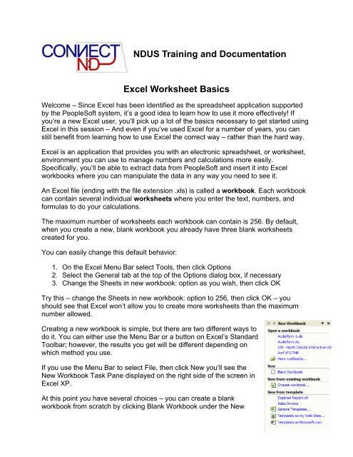
If you use the Menu Bar to select File, then click New you’ll see the
New Workbook Task Pane displayed on the right side of the screen in
Excel XP.
At this point you have several choices – you can create a blank
workbook from scratch by clicking Blank Workbook under the New

section, you can create a new workbook from an existing workbook by clicking Choose
workbook…, or you can create a blank workbook based on an existing template by
clicking a template under the New from template section.
If you’re using Excel 97 or Excel 2000, you’ll see the New dialog box on screen when
you choose File, New from the Menu Bar. In the New dialog box you can create a new
blank workbook by selecting the Blank Workbook icon, or you can create the new
workbook from an existing template by clicking the appropriate template icon.
A quicker way is to click the New Blank Document button on the Standard Toolbar to
immediately create a blank workbook without having to making selections in the Task
Pane or dialog box.
Once you’ve created your new workbook you’ll need to enter text, numbers (data), and
formulas and format the worksheets to look the way you want them. If you need to
increase or decrease the number of worksheets in the workbook you can easily add,
delete, copy, move, and rename any worksheet.
To delete a worksheet:
1. Click the worksheet tab (located at the bottom of the screen) you want to delete
to select it (the tab should appear highlighted in white)
2. Right-click the selected tab
3. Select Delete from the shortcut menu that appears
Just remember, any text or data that might be on the worksheet is deleted along with
the worksheet!
To add a new worksheet:
1. Click a worksheet tab to select it (the new worksheet tab will always be inserted
to the left of the selected worksheet tab)
2. Right-click the selected tab
3. Select Insert from the shortcut menu
4. Click the Worksheet icon (on the General tab in the Insert dialog box), then click
OK
To rename a worksheet:
1. Double-click the worksheet tab you wish to rename (tab text should appear in
reverse video)
2. Type the new name for the sheet, then press the Enter key
You can also move worksheets around within a workbook if you don’t like the order the
sheet tabs appear in at the bottom of the screen:
1. Click the worksheet tab you want to move to select it

2. Drag the worksheet tab to the right or left of the current location until you see a
small black triangle between the tabs where you
want to move the worksheet
3. Release the mouse button to move the sheet tab
If you’ve spent hours getting a worksheet just right, you can
copy that worksheet to create another worksheet without having
to “reinvent the wheel”:
1. Click the worksheet tab you want to copy to select it
2. Right-click the tab
3. Select Move or Copy… from the shortcut menu
4. Select the sheet you want located to the right of your
copied sheet in the Move or Copy dialog box
5. Check Create a copy, then click OK
Here’s a neat trick you can do with worksheet tabs, beginning with Excel XP – you can
color-code your worksheet tabs for easier viewing:
1. Click the sheet tab you wish to color to select it
2. Right-click the tab and select Tab Color…
3. Pick your color from the Format Tab Color dialog box, then click OK
Next we’ll take a look at the worksheet structure. Worksheets are arranged in columns
and rows. The intersection of a column and row is called a cell. Each cell is an
individual area where data (text, numbers, and formulas) can be entered. Each
worksheet contains 256 columns and 65,536 rows. If you multiply 256 columns x 65,536
rows x 256 worksheets, you can see that a workbook can potentially hold over 3 billion
individual cells of data!
Since there are so many cells to work with, it’s necessary to have a way of referencing a
particular cell. Each cell has a specific cell address defined by the column and row it
resides in.
Columns are labeled alphabetically from left to right starting with A. Columns to the right
of column Z are labeled starting with AA, AB and so on through all 256 columns.
Rows are labeled numerically from top to bottom starting with 1, continuing to row
65,536.
A cell address is noted first by its column letter (A, B, C, etc.) then its row number (1, 2,
3, etc.). A cell located in the third column from the left (C) in the fourth row down from
the top (4) is addressed as cell C4. You’ll use these cell addresses to navigate through
your worksheets, and you’ll use them to build formulas that produce calculations.

The selected cell (or the active cell) is always
marked by the cell pointer and the cell address is
shown in the Name box in the upper left corner
of the worksheet. The next thing you do (enter
data, issue a format command, etc.) will always
take place within the active cell indicated by the
cell pointer.
Name Box
Cell Pointer
There are several ways to navigate within your workbooks:
1. Use the Up, Down, Right, and Left Arrow keyboard keys to move the cell pointer
one cell up, down, right, or left at a time
2. Press the Enter key to move to the same cell in the next row down, press Shift +
Enter to move to the same cell in the next row up
3. Press the Tab key to move one cell to the right, press Shift + Tab to move one
cell to the left
4. Move the mouse pointer to the cell you want, then click the cell
5. Press the PgUp or PgDn keyboard keys to move one screen (not page) up or
down at a time
6. Press the Ctrl key + Home to move rapidly to the very first cell in the worksheet
(A1)
7. Press the Ctrl key + End to move rapidly to the last cell containing data in the
worksheet
8. Click in the Name box to select the current cell address, type
the cell address you want to go to (i.e. Z26) in the Name box,
then press the Enter key
9. On the Menu Bar, select Edit, click Go To…, type the cell address you want in
the Reference: text box, then click OK (Keyboard shortcut: Ctrl + G)
10. To move from worksheet to worksheet, click the sheet tab you want at the bottom
of the screen to activate it
11. Use the sheet tab navigation buttons at the bottom of
the worksheet to other worksheet tabs
Here’s a quick tip – When you save a workbook Excel “remembers” where the cell
pointer was currently located so the next time you open the file the cell pointer is right
where you left it. You can easily get “lost” in a large spreadsheet, but if you simply press
Ctrl+ Home before you save the file, the next time you open it you’ll be at the top, left
corner of the worksheet right away (cell A1).
You’ll also run into several different mouse pointer shapes in Excel and each one has a
very specific purpose. Make sure you are familiar with these shapes and know when to
use them:
o Large White Cross shape - Use to select a cell, or a range of
cells to affect them (apply formatting, enter
data, etc.)

o Small Black Cross shape – Use to Copy
(or Fill) cell contents to adjacent cells.
Appears when you point to the Fill
Handle
Mouse
Pointer
Fill
Handle
o White Slanted Arrow – Use to Move or Copy cell contents to
non-adjacent cells
• When you point to a border of the selected cell, this shape appears – click
and drag with the left mouse button to move the contents of the cell to
another non-adjacent cell – Hold down the Ctrl key, then click and drag with
the left mouse button to copy the cell contents to a non-adjacent cell
Row divider
Column divider
You can change the width of columns and rows if the column
width or the row height is too small or too large to display the
cell contents correctly. Position the mouse pointer on the
column or row divider line until you see a double-headed
arrow, then click and drag to the desired size – or better yet
– double-click the left mouse button on the divider line to
resize the column or row to the contents of the largest cell in
the column or row.
There’s a great shortcut if you need to quickly adjust all of the columns within a
worksheet to fit the contents of the widest cell in each column:
1. Click the Select All button in the upper-left corner of the worksheet to select the
entire worksheet
2. Double-click a column divider
In order to enter data, make changes to existing data, format cells and many other tasks
in Excel, you need to select the cell or cells you want to change. There are several ways
of selecting cells.
To select one cell, simply move the cell pointer to that cell
and it’s selected. Often you can make your work more
efficient if you select a range of cells before you take any
action. A range is a rectangular group of one or more
selected cells. When you select a range, any change you
make is applied to all of the cells in the range.
To select a range of adjacent cells, click the first cell you want to select, then drag down
and/or to the right to select adjacent cells. Release the mouse button when you’ve
selected the desired range. All of the selected cells in the range will be highlighted in
black (Excel 97) or blue (Excel 2000/2002). The cell containing the cell pointer (the

active cell) is displayed in white with a darker border, but it is still part of the selected
range.
To select multiple ranges select one range of cells
as you normally would, then hold down the Ctrl
key and click and drag to select the next range of
cells.
There are three different modes in Excel: Ready, Enter, and Edit. The mode indicator
appears on the Status Bar in the lower left corner of the Excel screen.
When a cell is selected but nothing has been entered into the cell, Excel is in Ready
mode and you see the word “Ready” displayed in the Mode area. The minute you press
any key (even the spacebar) to enter a character in the cell, Excel goes into Enter
mode. The word “Enter” is displayed in the status bar.
When Excel is in Enter mode many commands on the Menu Bar and buttons on the
toolbars are “grayed out” or not available until you exit Enter mode. In this mode, Excel
is waiting for you to Enter the cell contents by moving the cell pointer off the cell. You
can leave Enter mode in any of several ways:
1. Press the Enter key
2. Press the Tab key
3. Click another cell to select it
4. Use the arrow keys to move the cell pointer to another cell
While Excel is still in Enter mode the contents of the cell can still be canceled if you
press the Esc key in the upper left corner of the keyboard. Once you move the cell
pointer off the cell, the cell contents actually become part of the worksheet and you can
no longer cancel the entry; however, you can still delete or edit the cell.
When you’re back to Ready mode, you can click a cell to select it. The minute you start
typing, the existing cell contents are immediately replaced with the new data.
If you want to change a cell’s contents without deleting and retyping the entire entry,
you can use Excel’s Edit mode. Select the cell, then press the F2 key (or double-click
the cell). You will see the word “Edit” displayed in the Mode area on the Status Bar.
While in Edit mode, the cell pointer changes into a blinking cursor you can move to the
area to be changed. Move the cell pointer to another cell to accept your changes and
return Excel to Ready mode.
Now we’ve come to the real reason people use Excel – creating formulas to calculate
numbers! One of the reasons Excel is such a popular application is its ability to do
automatic recalculation. When you have created formulas in your worksheets, and you

make changes to cells that your formulas reference, all formula results are automatically
recalculated immediately when the cell pointer leaves the changed cell.
To produce calculations, you could simply select a cell and type in constant values from
other cells like the example on the left:
Both of these
formulas produce
the same results
While the formula on the left does work, it doesn’t allow you to make changes easily
later. For this reason, you will most often use cell references (i.e. A1, C2, etc.) in your
formulas rather than constant values, as in the example on the right.
To build a formula, select the cell where you want the result to appear, then type the =
symbol to begin the formula. You can enter your cell references in one of two ways:
1. Type the cell reference(s) and mathematical operators manually
2. Click on the cell(s) you want to reference with the mouse, and type the necessary
operators
As you enter your formula, you can see the
formula displayed in the Formula Bar. When you
move the cell pointer to another cell, the formula is
entered and the formula’s result displays in the
cell. To see the formula again, select the cell and
look at the formula bar.
Excel produces calculations from formulas based on the actual values entered into the
cells referenced by the formula. The values you see displayed in a cell may differ from
the cell’s actual contents which a formula is using. For example, you may enter 10.059
as the value in a cell, but the cell may be formatted to display only two decimal points.
The cell display shows 10.06, but the actual value used in formulas would be 10.059!
To compare a cell’s actual contents to the displayed
value, simply select the cell and then look at the
Formula Bar. This may eliminate a lot of confusion and
problems!
Mathematical Operators used in formulas:
+ Addition
- Subtraction
* Multiplication
/ Division
^ Exponentiation (2 10 )

Excel uses the standard mathematical operator precedence rules to determine the
order in which calculations are performed when more than one operator is used in the
same formula. For example, the following two formulas produce completely different
results because of operator precedence:
=562/2 + 126 * 2 3 = 1289 =(562/2 + 126) * 2 3 = 3256
Operator precedence (or Order of Operations) means that operators used within the
same formula will be performed in this order:
1. Parentheses
2. Exponentiation (2 10 )
3. Multiplication/Division
4. Addition/Subtraction
Here’s a quick way to remember the order of operations: “Please Excuse My Dear Aunt
Sally” or PEMDAS!
So, what do you do if you want to include more than one cell in a cell reference in a
formula? All you need to do is indicate a range of cells in your formula like this:
A1:B5
This range includes all cells beginning with cell A1 through A5 and B1
through B5
Excel has over 200 built-in functions that make building your formulas easier.
Functions are formulas that have already been built for you – all you need to do is
supply the correct cell references.
You can create formulas using functions in several ways:
• Type the formula using a function manually
• Use the Paste Function (Excel 2000) or the Insert Function (Excel XP) button to
let Excel build the formula for you
• For commonly used functions, use the buttons supplied on Excel’s Standard
Toolbar

One function almost all Excel users will use frequently is the SUM
function to produce the sum of a range (or multiple ranges) of cells
without typing each cell reference and the + symbol.
This function =SUM(A1:A3) produces the same results as =A1+A2+A3
Since the SUM function is used so frequently, you can use the Sum
button to speed things up. Select the cells you wish to add, including the blank cell
where you want to place the total, then click the Sum button. The formula will be
=SUM(A1:A5) and the result will be calculated in cell A6.
To use the Paste Function (2000) or Insert Function (XP) feature, place the cell pointer
in the cell where you want the formula to appear, then click the Paste Function button
on the Standard Toolbar (2000), or the Insert
Function button on the Formula Bar (XP).
In the Insert Function dialog
box you can search for a
particular function (i.e.
Average) in the Search text
box, or you can select a
category from the Or select a
category: drop-down list then
click the function you want to
use from the Select a
function: list box.
Once you’ve selected a
function you’ll see the
function’s correct syntax and
a description of the function at
the bottom of the dialog box
and you can learn more about
the function under Help on
this function.
Click OK to go to the next
step.
Enter the cell references
and operators to build the
formula in the Function
Arguments text boxes,
then click OK. You’re
done!