Text anzeigen (PDF) - Universität Duisburg-Essen

32 2. Theoretical background
(a)
relative energy
1.0
0.5
0.0
−0.5
−1.0
p-core levels
Fe 2p
−1/2
−1.5
1/2
0.0 0.2 0.4 0.6 0.8 1.0
relative spin‒orbit λ
coupling strength, λ + ζ
m j
3/2
1/2
−1/2
−3/2
(b)
1.0
0.5
0.0
d-core levels
5/2
3/2
1/2
−1/2
−3/2
−5/2
−0.5
3/2
−1.0
1/2
−1/2
Gd 4d
−3/2
−1.5
0.0 0.2 0.4 0.6 0.8 1.0
relative spin‒orbit λ
coupling strength, λ + ζ
m j
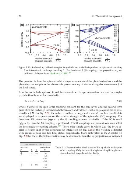
Figure 2.20.: Reduced m j sublevel energies for p-shells and d-shells dependent on spin–orbit coupling
λ or intra-atomic exchange coupling ζ. For dominant λ (jj coupling), the projections m j are
indicated. Adapted from Henk et al. (1999). 87
The question is, how the spin and orbital angular momenta of the photoionized core and the
photoelectron couple to the observable projections m J of the total angular momentum J of
the final states.
In order to include spin–orbit and intra-atomic exchange interaction, we use the singleparticle
Hamiltonian for core-shells,
H = λ(l·σ) + ζσ z , (2.34)
where λ denotes the spin–orbit coupling constant for the core-level, and the second term
quantifies the exchange interaction between core and valence-level along a quantization axis,
usually z ‖ M. In Fig. 2.20, the reduced sublevel energies of p and d core-level multiplets
are displayed in dependence on the relative strength of the spin–orbit (SO) coupling. For
dominant SO interaction (
λ+ζ λ ≈ 1), the jj coupling scheme is suitable. If the SO is small
≈ 0), then the LS-coupling is preferred. If both couplings are present, one may select
( λ
λ+ζ
the intermediate coupling scheme. 109 There exist simple cases, in which e. g. the Fe 2p orbital
is clearly split by the dominant SO interaction (in Fig. 2.20a), this yielding a doublet
with groups of four and two final states, respectively. More ambivalent is the d orbital (in
Fig. 2.20b). Here, the SO interaction may be dominant, then the m J projections as indicated
only spin–orbit j = + s ∗ .
core hole
projection
s ∗ j m j
+ 1 2
1 3/2 3/2
1/2
−3/2
−3/2
Table 2.1.: Photoemission final states of Eu np shells with spin–
orbit coupling. Only intra-orbital spin–orbit splitting is considered,
which is applicable for Eu 3p.
− 1 2
1 1/2 1/2
−1/2