Skopje, Makedonija INTERPOLATION POLYNOMIALS VIA AIFS 1 ...

70 LJ. KOCIĆ, S. G-ZAJKOVA, V. ANDOVA
where
[
m L (x) = 1
x − a
c − a
( ) 2 x − a
...
c − a
( ) n
] T
x − a
c − a
is the ”left” monomial basis, coincides with P n (x) on the left subinterval [a, c],
and, at the same time, the ”right” polynomial
Pn R (x) =(a R ) T · m R (x), x ∈ [c, b]
where
[
m R (x) = 1
x − c
b − c
( ) 2 x − c
...
b − c
( ) n
] T
x − c
b − c
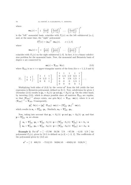
coincides with P n (x) on the right subinterval [c, b]. In fact, it is a binary subdivision
problem for the monomial basis. Now, the monomial and Bernstein basis of
degree n are connected by
m(x) =T BM · b(x) (3.3)
where T BM is an n × n upper-triangular matrix of the form (for n =1, 2, 3and4)
⎡
⎤
⎡
[ ] 1 1
[1] ,
, ⎣ 1 1 1
⎤ 1 1 1 1 1
0 1/4 1/2 3/4 1
0 1/2 1 ⎦ ,
0 1
⎢ 0 0 1/6 1/2 1
⎥
0 0 1 ⎣ 0 0 0 1/4 1 ⎦ , ...
0 0 0 0 1
Multiplying both sides of (3.3) by the vector a T from the left yields the last
expression is Bernstein polynomial, defined on [0, 1]. Now, subdivision for given λ
(formulae (2.4)) results in p L = S L (λ) · p and p R = S R (λ) · p. On the other hand,
by inverting (3.3), which is always possible since all matrices T BM are regular,
so that (T BM ) −1 always exists, one gets b(x) = T MB · m(x), where it is set
(T BM ) −1 = T MB . Consequently,
p T L · b(x) = ( p T ) ( )
L · T MB · m(x) = T
T T
MB · p L · m(x),
which results in a L = T T MB · p L. Similarly, a R = T T MB · p R.
Now, taking into account that p L = S L (λ) · p and p R = S R (λ) · p, andthat
p = T T BM · a, we obtain
{
aL = T T MB · p L = T T MB · S L(λ) · p = ( T T MB · S )
L(λ) · T T BM · a =AL · a
a R = T T MB · p R = T T MB · S R(λ) · p = ( T T MB · S R(λ) · TBM) T · a =AR · a
Example 2. For ā T = [ −17/90 59/36 7/9 −97/36 −4/45 5/9 ] the
polynomial P n (x), given by (3.1) is defined on [a, b] =[−2, 2]. The coefficients of
the polynomial given by (3.2) are
a T = [ 2 809/15 −7112/15 58288/45 −65024/45 5120/9 ]