Skopje, Makedonija INTERPOLATION POLYNOMIALS VIA AIFS 1 ...
Skopje, Makedonija INTERPOLATION POLYNOMIALS VIA AIFS 1 ...
Skopje, Makedonija INTERPOLATION POLYNOMIALS VIA AIFS 1 ...

You also want an ePaper? Increase the reach of your titles
YUMPU automatically turns print PDFs into web optimized ePapers that Google loves.
<strong>INTERPOLATION</strong> <strong>POLYNOMIALS</strong> <strong>VIA</strong> <strong>AIFS</strong> 71<br />
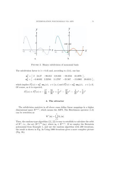
a. b.<br />
Figure 2. Binary subdivision of monomial basis<br />
The subdivision factor is λ =0.45 and, according to (3.4), one has<br />
a T L = [ 2 24.27 −96.012 118.033 −59.2531 10.4976 ] ,<br />
a T R = [ −0.46432 2.22581 11.2707 −25.567 −15.0965 28.6313 ] ,<br />
which implies Pn L (x) =a T L ·m L(x), x ∈ [a, c] andPn R (x) =a T R ·m R(x), x ∈ [c, b].<br />
Of course, as it is expected,<br />
Pn L (x) ≡ Pn R (x) ≡− 17<br />
90 + 59<br />
36 x + 7 9 x2 − 97<br />
36 x3 − 4<br />
45 x4 + 5 9 x5<br />
4. The attractor<br />
The subdivision matrices in all above cases define linear mappings in a higher<br />
dimensional space R m+1 , which means the <strong>AIFS</strong>. The Hutchinson operator (1.3)<br />
can be rewritten as<br />
n⋃<br />
W ′ (x) = S i (x)<br />
Then, the random-type algorithm ([1], [2]) is easy to establish to calculate the orbit<br />
of W ′ , i.e., the set (W ′ ) ◦m (x 0 ), where x 0 ∈ R m+1 . If we employ the Bernstein<br />
polynomial from Example 1, and use the random algorithm with 200 iterations,<br />
the result is shown in Fig. 3a Using 1000 iterations gives a more complete picture<br />
(Fig. 3b).<br />
i=1