Fractional and operational calculus with generalized fractional ...

806 Ž. Tomovski et al.
Downloaded By: [Srivastava, Hari M.] At: 18:19 27 October 2010
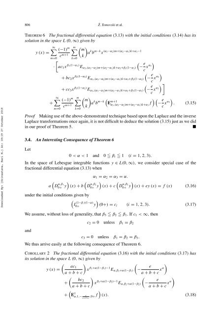
Theorem 6 The fractional differential equation (3.13) with the initial conditions (3.14) has its
solution in the space L (0, ∞) given by
∞∑ (−1) m ∑
m ( ) m
y (x) =
a k b m−k x (α 3−α 2 )m+(α 2 −α 1 )k+α 3 −1
k
m=0
+
·
c m+1
k=0
[
ac 1 x β 1(1−α 1 ) E α3 ,(α 3 −α 2 )m+(α 2 −α 1 )k+α 3 +β 1 (1−α 1 )
∞∑
m=0
+ bc 2 x β 2(1−α 2 ) E α3 ,(α 3 −α 2 )m+(α 2 −α 1 )k+α 3 +β 2 (1−α 2 )
+ cc 3 x β 3(1−α 3 ) E α3 ,(α 3 −α 2 )m+(α 2 −α 1 )k+α 3 +β 3 (1−α 3 )
(−1) m
c m+1
m ∑
k=0
(
− e )
c xα 3
(
− e )
c xα 3
(
− e ) ]
c xα 3
( ) m ( )(
a k b m−k E m+1
α
k 3 ,(α 3 −α 2 )m+(α 2 −α 1 )k+α 3
f − e )
c xα 3
. (3.15)
Proof Making use of the above-demonstrated technique based upon the Laplace and the inverse
Laplace transformations once again, it is not difficult to deduce the solution (3.15) just as we did
in our proof of Theorem 5.
3.4. An Interesting Consequence of Theorem 6
Let
0