Download as a PDF - CiteSeerX

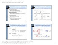
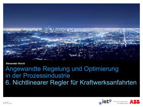
Alexander Horch
Angewandte Regelung und Optimierung
in der Prozessindustrie
6. Nichtlinearer Regler für Kraftwerksanfahrten
© A.Horch
SS 2010 | Slide 1

Kraftwerksautomatisierung
Einführung
• Prinzipiell ist ein Kraftwerk einer chemischen
Prozessanlage ähnlich. Es gibt jedoch einige Spezifika,
weshalb das Gebiet der Kraftwerksautomatisierung sich als
eigenständiger Zweig entwickelt hat.
• Kraftwerke haben eine Lebensdauer von ca. 40 Jahren.
• Bis 2020 werden ca. 50 neue Kraftwerke in Deutschland
geplant.
• Durch zunehmende Integration erneuerbarer
Energiequellen wird das Elektrizitätsnetz in Deutschland
komplexer und damit steigen die Anforderungen an
Kraftwerke und ihren Betrieb.
© ABB Group
SS 2010 | Slide 2

Kraftwerke
Grundprinzipien
• Herzstück ist der Generator
• Basiert auf dem dynamoelektrischen Prinzip (W.v. Siemens,
1866)
• Wandelt mechanische in elektrische Energie
• Der größte Teil sind jedoch die Dampferzeugung und die
Reduzierung der Umweltbelastungen
• Die Automatisierung elektrischer Übertragungs- und Verteilnetze
ist eine eigenständige Disziplin, die sich von der
Kraftwerksautomatisierung stark unterscheidet.
• Dampfkraftwerke werden seit 40 Jahren verbessert, in der wurde
der Wirkungsgrad um ca. 1/3 gesteigert.
• Weiterhin wurden massive Verbesserungen im Umweltschutz
erreicht (z.B. Rauchgasreinigung)
• Die Möglichkeiten zur Verbesserung sind noch nicht ausgeschöpft.
© ABB Group
SS 2010 | Slide 3

Kraftwerkstypen
Konventionelle Kraftwerke
• Dampfkraftwerke
• Antrieb des Generators durch Dampfturbine; eine
Sonderform der Dampfkraftwerke sind Heizkraftwerke,
die sowohl Strom erzeugen als auch Wärme
auskoppeln
• Gasturbinenkraftwerke
• Antrieb des Generators durch Gasturbine
• Kombikraftwerke
• Antrieb der Generatoren durch Gas- und Dampfturbine
• Block(heiz)kraftwerke
• Antrieb des Generators durch Verbrennungsmotor
• Kernkraft, Wasserkraft, Windkraft, Solar, Biomasse, ...
© ABB Group
SS 2010 | Slide 4

Kraftwerke
Wirkungsgrade
• Wirkungsgrad η = Verhältnis von abgegebener Leistung
(P Nutzen
) zu zugeführter Leistung (P Aufwand
)
• η = [0...100%[. η > 100% ist ein Perpetuum Mobile.
• Carnot-Wirkungsgrad
kann niemals überschritten werden
Wirkungsgrad einer
Glühlampe
• Kohlekraftwerke heute: Max. Dampftemperatur T~600 °C (η~45%)
• Es werden Versuche gemacht, T~700 °C zu erreichen.
T n – niedrigste, T h – höchste Temperatur [K]

Wirkungsgrade in der Technik

Kraftwerksbetrieb
• Man unterscheidet
• Grundlastkraftwerke: laufen kontinuierlich
• Mittellastkraftwerke: laufen meist
• Spitzenlastkraftwerke: laufen bei Bedarf
© ABB Group
SS 2010 | Slide 7

Fossile Dampfkraftwerke
Charakteristika
• Häufigster Kraftwerkstyp (‚Arbeitspferd‘ der
Energiewirtschaft)
• Kraftwerke sind mit einigen Varianten weitgehend ähnlich
in Betrieb und Komponenten
• Durch gesetzliche Auflagen sind Kraftwerke vielfältig
instrumentiert.
• Großer Aufwand wird in die Rauchgasreinigung gesteckt.
• Durch verschiedene Zwischenüberhitzungen kann der
Wirkungsgrad gesteigert werden. Der theoretisch mögliche
Wirkungsgrad des Carnot-Prozesses ist noch nicht
erreicht.
• Basisregelungen ebenso wie gehobene Regelungen
spielen eine große Rolle im Erreichen moderner
Wirkungsgrade.

Dampfkraftwerk
Funktionsweise
Meist fossile Energiequellen:
• Braunkohle
• Steinkohle
• Erdöl
Wasser-Dampf-Kreislauf:
Der Dampf wird nach dem
Austritt aus der Turbine
zu Wasser kondensiert.
© ABB Group
SS 2010 | Slide 9

Dampfkraftwerk
Funktionsweise
© ABB Group
SS 2010 | Slide 10
REA - Rauchgasentschwefelungsanlage

Dampfkraftwerk
Funktionsweise
© ABB Group
SS 2010 | Slide 11

Dampfkraftwerk
Funktionsweise
Der zum Betrieb der Dampfturbine notwendige Wasserdampf wird in einem
Dampfkessel aus zuvor gereinigtem und aufbereitetem Wasser erzeugt. Durch
weiteres Erwärmen des Dampfes im Überhitzer nimmt die Temperatur und
das spezifische Volumen des Dampfes zu. Vom Dampfkessel aus strömt der
Dampf über Rohrleitungen in die Dampfturbine, wo er einen Teil seiner zuvor
aufgenommenen Energie als Bewegungsenergie an die Turbine abgibt. An die
Turbine ist ein Generator angekoppelt, der die mechanische Leistung in
elektrische Leistung umwandelt. Danach strömt der entspannte und
abgekühlte Dampf in den Kondensator, wo er durch Wärmeübertragung an die
Umgebung kondensiert und sich als flüssiges Wasser an der tiefsten Stelle
des Kondensators sammelt. Über die Kondensatpumpen und den Vorwärmern
hindurch wird das Wasser in einen Speisewasserbehälter
zwischengespeichert und dann über die Speisepumpe erneut dem
Dampfkessel zugeführt.
© ABB Group
SS 2010 | Slide 12

Exemplary Water-Steam Cycle
DT Kugelstück (Innen- und Mittelfaser
03RA05T002I und 03RA05T002M)
FD-Menge
RA07F901
FD-Temperatur
RA07T901
Ü V
EK IV/1
Ü IV
Ü III
EK II/1
Dampftemp
nach Ü V
RA01T004
Temp
Dampftemp
EK IV/1
Dampftemp
vor EK IV/1
Dampftemp
vor EK III/4
Dampftemp
nach EK II/1
Dampftemp
vor EK II/1
Ü V
RG-Temp v Ü V
NR05T010 und 20
RV EK IV/1
EK IV/4
Dampftemp. vor
EK IV/4 NA44T004
Ü IV
RG-Temp v Ü IV
NR04T010 und 20
Dampftemp vor EK
III/4 NA34T004
RV EK II/1
2
Ü II
Ü III
EK II/4
Dampftemp vor EK II/4
NA24T004
Dampftemp nach
Ü V RA04T004
4
Dampftemp nach
EK IV/4 NA44T008
6
Dampftemp nach
EK II/4 NA24T008
FD-Druck
RA07P901
RV EK II/4
RL24S002
RV EK IV/4
RL44S002
DT Sammler IV/4 (Innen- und
Mittelfaser NA44T010I und NA44T010M)
3 Kombination Strahlung/Konvektion
DT Sammler III/4 (Innen- und Mittelfaser
NA34T010I und NA34T010M)
DT Sammler II/4 (Innen- und Mittelfaser
NA24T010I und NA24T010M)
Stellungsbefehl Y
HDU 1...4 RA08C000
RA 80
Druck kalte ZÜ
RC12P007
ZÜ I
7
DT Hosenstück (Innen- und Mittelfaser
03RA07T003I und 03RA07T003M)
HD
HD-Einlaß-RV Turbine
SA11S016-46
Generatorleistung
SP10E927
MD-RV
Turbine
Anordnung ist 4-strängig
(4 HDUs, 4 HD-Turbinen-
RV)
Radkammerdruck
SA11P020
MD/
ND
MDU
G
Hauptentwässerungen
zu den Abscheidern 1 - 3
Dampftemp n EK I/1
NA11T007
RV EK I/1
RL11S002
EK I/1
Verdampfer
Verdampfermenge
NA01F001
Temp Speisesewasser vor
Verdampfer NA01T001
Dampftemp vor
EK I/2 NA12T007
Eco
1
EK I/2
RV EK I/2
RL12S002
Ü I
Umwälzmenge
NB05F901
ECO Speisew.-
Menge RL15F001
Dampftemp nach
Abscheider 4 NA16T005
Abscheider
4
pD Anfahrflasche NB01P003
Niveau Anfahrflasche
NB01L901
Summe Menge
Notabläufe RK10F001
SPW-Pumpe
1 8
ZÜ II
5
Zwischenüberhitzer (ZÜ)
rauchgasseitige Reighenfolge
der Überhitzer
SPW-
Behälter
Kondensatpumpe
ND-
Vorwärmer
© ABB Group
SS 2010 | Slide 13
8
Temp Speisew vor ECO
RL15T004
HD-Vorwärmer
SPW-Druck vor HD-
Vorwärmer
RL10P002

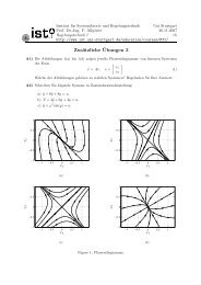
Exkurs
Zukunftsprojekt ‚Desertec‘

Exkurs
Zukunftsprojekt ‚Desertec‘
• Die Energie für die
Überhitzung des
Wasserdampfes entsteht
aus durch
Sonnenkollektoren
erhitztem Öl.
• Der Rest entspricht genau
einem Dampfkraftwerk.

Typische Suite von gehobenen Lösungen für Kraftwerke
Beispiel ABB Optimax TM

Kraftwerksautomatisierung – Kessel
Was muss geregelt werden?

Kraftwerksautomatisierung – Kessel
Bespiel Verbrennungsoptimierung
Manipulated variables
• Air dampers at every burner
• Overfire air dampers
• Total air flow
• F primary air
• F secondary air
• Flue gas recirculation
• feeder / fuel oil flow
Process-/disturbance variables
• Coal / fuel oil quality
• Mill / burner wear
• Boiler cleanliness
• Ambient conditions
Boiler
Controlled
variables
• Flue Gas Boiler Exit
• O 2 concentration
• Exhaust Gas temperature
• NO x concentration
• CO concentration
• Carbon in Ash

Kraftwerksautomatisierung – Kessel
Bespiel Verbrennungsoptimierung

Kraftwerksautomatisierung – Kessel
Bespiel Verbrennungsoptimierung
• Max limit lowered sequentially by 10 ppm from 225 to 195
NOx
(ppm)

Kraftwerksautomatisierung
Closed-loop Energy Management and Coordinated Control
Example improved control of steam Temperature, Flow,
Pressure:
• T 1.2% of energy cost savings
• F 3% of energy cost savings
• p standard deviation reduced from 88 to 18kPa
• Less thermal cycle stress on the high pressure parts
• More stable operation, less boiler trips
• Less operator intervention required

Warum Kesselanfahrt optimieren?

Warum Kesselanfahrt optimieren?

Kesselanfahrtoptimierung
Motivation
• Warum Anfahrtoptimierung?
• Schnelle Anfahrt in definierter Zeit
• Einsparung von Öl und Kohlestaub
• Einhalten der Grenzen des thermischen Stresses
• Was für eine Regelung / Optimierung braucht man?
• Vermutlich nicht-linear, da Anfahrt einen großen
Arbeitsbereich durchläuft (Linearisierung nicht möglich)
• Randbedingungen müssen eingehalten werden können
(thermischer Stress)
• Möglichkeit, verschiedene Gütekriterien vorzugeben
(Zeit, Energieverbrauch, Schonung)

NMPC: Minimizing Thermal Stress at Boiler Start-up
Configuration of a heat recovery steam
generation plant
Thick-walled steam header (cylindric type, 6.4 cm thick)
Superheater
subsystems
Stretching of the material
because of temperature gradients
lead to lifetime reduction
© ABB Group
SS 2010 | Slide 25

Kesselanfahrt
Modellbildung
• Statische Modelle: verfügbar zur Auslegung aber ohne
Dynamik zur Regelung nicht geeignet.
• Daten-getriebene Black-box Modelle: nur geeignet für den
Einsatz in einem Arbeitspunkt. Nicht physikalisch.
• Physikalische Modelle: Aufwändig, komplex, physikalisch.
• Balance zwischen Genauigkeit und Beherrschbarkeit
• Modelle für Regelungsaufgaben müssen nur die
wichtigsten Dynamiken beschreiben, da die Regelung
Unsicherheiten quasi ausgleicht.
• Für Designaufgaben sind genauere Modelle notwendig.

Kesselanfahrt
Model building principles
• Drum level control (DLC)
• important problem in power plant
• ~30% of shutdowns due to poor level control of steam
water level in DLC
• difficult control problem due to shrink and swell
dynamics non-minimum phase behaviour
feed water q f
saturated steam q s
Reality: complicated
geometry with many
downcomer and
riser tubes.
heat Q
drum level

Kesselanfahrt
Model building principles
• This setup has a very efficient heat transfer due to boiling
and condensation.
• All parts of the system which are in contact with the
saturated liquid-vapor mixture will be in thermal equilibrium.
• Energy stored in the system and water is released or
absorbed very rapidly when the pressure changes.
• The rapid release of energy ensures that different parts of
the boiler change their temperature in the same way.
• Therefore low-order dynamics are sufficient!
• Model consits fo global mass and energy balances.

Kesselanfahrt
Model building principles
• System inputs
• heat flow rate to risers Q
• feedwater mass flow rate q f
• steam mass flow rate q s
• System outputs
• drum pressure p
• drum water level l
• Parameters / Variables
• volume (V), specific density (ρ), specific internal energy
(u), specific enthalpy (h), temperature (t), total mass of
metal tubes and the drum (m t
), specific heat of metal
(C p
)

Kesselanfahrt
Simple boiler model
• Global mass balance:
d
dt
[ ρs
Vst
+ ρw
Vw
] = q
f
− qs
Subscripts:
s – steam
w – water
f – feedwater
m – metal
t – total system
d – drum
r – risers
• Global energy balance (with u = h – p/ρ):
d
dt
[ ρ
]
s
hs
Vst
+ ρw
hw
Vw
− pVt
+ mt
C
p
tm
= Q + q
f
h
f
− qshs
• Total volume of the drum, downcomer and riser V t :
V t
= V st
+ V wt
• Steam tables for saturated
steam
• use of quadratic approximations
proved sufficient

Kesselanfahrt
Simple boiler model
• This model is a differential algebraic system (DAE)
• Such a model can be used for direct simulation.
• There are many different choices for state variables, e.g.
• drum pressure p, total volume of water V wt
• The model can then further be simplified
• Further model equations (to obtain drum level)
• Riser: heated tube with water / steam
• Essential to capture amount of steam in the risers
• Mass & energy balances for risers

Alexander Horch
Objekt-orientierte Modellierung
MODLICA
© A.Horch
SS 2010 | Slide 32

Modelica Overview by Martin Otter
Abstract:
This slide set gives an overview about the Modelica language,
including users view, libraries and a sketch of the language elements.
Copyright © 2005-2009, Martin Otter.
This material is provided "as is" without any warranty. It is licensed under the
CC-BY-SA (Creative Commons Attribution-Sharealike 3.0 Unported) License,
see http://creativecommons.org/licenses/by-sa/3.0/legalcode
Modelica® is a registered trademark of the Modelica Association

1. Modelica Introduction
Goal of Modelica:
• Modeling the dynamic behavior of technical
systems consisting of components from, e.g.,
mechanical, electrical, thermal, hydraulic,
pneumatic, fluid, control and other domains
in a convenient way.
• Models are described by
differential, algebraic, and discrete equations.
• No description by partial differential equations, i.e.,
no FEM (finite element method) and
no CFD (computational fluid dynamics),
but using results of, e.g., FEM programs.
• Modelica is used in industry since year 2000.

Example: detailed vehicle model
• Vehicle dynamics (3-dim. mechanics)
• Drive trains (1-dim. mechanics)
courtesy: Modelon AB
• Hydraulics
• Combustion
• Air Conditioning
(Thermofluid systems)
• Electrical/electronic systems
• Electrical machines
courtesy Modelon AB
• Hierarchical state machines
• Control (Input/output blocks, ...)

Modelica Language und Simulation-Environments
Graphical editor
for Modelica models
Modelica simulation
environment
(free or commercial)
Textual description
on file (equations,
"schematic", animation)
Free Modelica language
Translation of Modelica
models in C-Code,
Simulation, and
interactive scripting
(plot, freq. resp., ...)
Modelica Simulationenvironment
(free or commercial)

Commercial Modelica Simulation Environments (alphabetical list)
• CATIA Systems from Dassault Systèmes
(based on Dymola kernel with PLM integration)
• Dymola from Dynasim AB, Sweden
(Dynasim was acquired by Dassault Systèmes in 2006).
• LMS Imagine.Lab AMESim from LMS International
• MapleSim from MapleSoft, Canada.
• MathModelica from MathCore AB, Sweden.
• SimulationX from ITI GmbH, Dresden, Germany.
Free Modelica Simulation Environments (alphabetical list)
• OpenModelica from Linköping University, Sweden
(under development; subset of Modelica is available)
• SCICOS from INRIA, France
(under development; subset of Modelica is available).
An up-to-date list of Modelica tools is available from www.modelica.org/tools

Modelica Association
• Modelica is a free language and is developed by the (non-profit)
Modelica Association since 1996
2000: First applications
...
2005: Modelica 2.2
2007: Modelica 3.0
2009: Modelica 3.1 (actual)
• Develops also the largest, free library
for multi-domain models
(Modelica Standard Library)
62 nd Design Meeting in Lund, May 2009
(after release of Modelica 3.1)
• 80 "individual" and 11 "organizational members"
(interested in "active" individual members; Therefore requirement:
participation at 2 Modelica Design Meetings in the last 12 months).
• 6 International Modelica Conferences (Modelica'2008 with 250 participants)
• All infos under http://www.Modelica.org
(Specification, simulation environments, free libraries, 300 papers, ...)

Example: Industrial Robots (from Modelica.Mechanics.MultiBody.Examples.Systems.RobotR3.fullRobot)
model Resistor
extends OnePort;
parameter Real R;
equation
v = R*i;
end Resistor;
1000 non-trivial algebraic equations, 80 states.
Faster as real-time on slow PC.

Example: Hardware-in-the-Loop Simulation of automatic gear boxes
(different vehicle manufacturers)
Electronic Control Unit
(Hardware)
desired pressure
(Simulation)
+ driver + engine
+ 1D vehicle dynamics

More free libraries under www.Modelica.org/libraries

Quickly growing number of commercial libraries. Small selection:
SmartElectricDrives (ATI, Austria)
Controlled electrical machines with quasi-stationary and
transient models, e.g.,
controllers (voltage/frequency, field-oriented, speed/position),
power electronics (AD/DC, DC/AC, DC/DC converters, PWM),
energy storages (batteries, supercaps, fuel cells), ...
Hydraulic/Pneumatic Libraries (Modelon AB, Sweden)
Libraries to model pipe networks for oil and air. Contain all
important standard components like pumps, valves,
volumes, lines, sensors
PowerTrain (DLR-RM, Germany)
Library to model vehicle power trains and all type of
planetary gearboxes. E.g. standard and planetary
gears with losses, clutches with friction, flexible
driveline models, automatic gearboxes,
optional 3D effects (mounting on vehicle)

Modelica Language Elements
Example: Definition of Capacitor
connector Pin
Voltage v; // identical at connection
flow Current i; // sums to zero at connection
end Pin;
partial model TwoPin
Pin p, n; Voltage v;
equation
v = p.v - n.v;
0 = p.i + n.i;
end TwoPin;
model Capacitor
extends TwoPin;
parameter Capacitance C;
equation
C*der(v) = p.i;
dv
end Capacitor;
dt

Object-oriented modeling
• Graphical flowsheet modeling
• Combine commodity models with proprietary knowledge
• Automatic generation of stand-alone executable code
© ABB Group
SS 2010 | Slide 44

Object-oriented modeling
• Graphical modelling
• Connections are non-direction connections. Concerned variables
are either equal or sum up to zero (e.g. force – velocity; current –
voltage)
• Done by the modelling tool (e.g. Dymola*)
• Read model files and collect equations from sub-models
• Generate connection equations considering Kirchhoff‘s laws,
analyse causality
• Detect and treat DAEs, index reduction
• Change equations for unknown variables
• detect and tread algebraic loops analytically
• determine state variables, create an ODE if possible
• generate target code for numerical solvers (e.g. Simulink S-
function)
© ABB Group
SS 2010 | Slide 45
*www.dynasim.se

Boiler Modelling
The final model
• Implicit DAE System with 538 unknowns and 538
equations of the form
•
⎡
⎤
S
⎢
x( t),
x(
t),
y(
t),
u(
t),
v(
t),
p
⎥
= 0
⎣
⎦
x – state variables
y – output variables
u – manipulated variables
v – algebraic variables
p – constant parameters
• Symbolic equation processing (Dymola) eliminates 352
connection variables, and other things, resulting to:
•
∧
x( t)
= f
, x(
t0)
= x0
y(
t)
= g
( x(
t),
u(
t),
p)
( x(
t),
u(
t),
p)
• This is an explicit ODE with only eight states.
• Initial conditions and parameters need to be estimated from
data.

Dynamic optimization problem
J
s.
t.
t
f
[ T(
t)
−T
= ∫ 2
w
t=
0
x&
( t)
=
T
f [ x(
t),
q
set
F
]
2
( t),
Y
[ p(
t)
− p
+
2
w
HPB
p
( t),
Y
AW
set
]
2
( t)],
[ q
+
m
( t)
−q
w
2
q
m
x(0)
= x
m,
set
]
2
dt
⎯→
‣ Process model
q
F
min
( t),
Y
HPB
( t)
q
F,min
0 ≤Y
≤ q
HPB
F
≤ q
( t)
≤1
F,max
,
q&
F,min
≤ q&
F
≤ q&
F,max
‣ bounds on fuel
‣ bounds on valve positions
ΔT
min, i
≤ ΔT
( t)
≤ ΔT
i
max, i
,
i
= 1,..., n
‣ thermal stresses
General startup optimization problem:
Optimal transition to new operating point (T,p,q m ) subject to control bounds and state constraints (esp.
thermal stresses).
© ABB Group
SS 2010 | Slide 47

Discretization of the optimization problem
• Parameterize control u(t) = u(u k ), k=0,1,…,K-1
• Convert dynamic optimization problem to discrete-time optimal control
problem:
J
=
s.
t.
x
c
c
k+
1
k
K
( x
f
( x
K−1
K
k k
0(
x ) + ∑ f0(
x , u
0
x , u
k=
0
=
k
, u
K
f
k
k
( x
) ≥ 0,
) ≥ 0
k
, u
k
),
) ⎯→min
k = 0, K,
K −1
k = 0, K,
K −1
• Solve as large-scale nonlinear programming
problem with vector of optimization variables v:
k
0
⎛ x
⎜
0
⎜ u
⎜ 1
⎜
x
1
⎜ u
v = ⎜
⎜ M
⎜
K
x
⎜
K
⎜u
⎜ K
⎝ x
−1
−1
⎞
⎟
⎟
⎟
⎟
⎟
⎟
⎟
⎟
⎟
⎟
⎟
⎠
© ABB Group
SS 2010 | Slide 48

Modellprädiktive Regelung
Prinzip

Optimierungslösung

Optimization solver
Huge Quadratic Programming (HQP)
• HQP is a solver for nonlinearly constrained
large-scale optimization. It is primarily intended
for the optimization of dynamic systems.
• HQP is implemented as framework in C++.
External model interfaces are provided for
Simulink S-functions.
• HQP uses a sparse interior point algorithm for
the efficient treatment of the linear-quadratic
subproblems in the nonlinear SQP iterations.
• HQP combines a large-scale nonlinear
optimization solver with ODE and DAE solvers.
TCL – tool command language (www.tlc.tk)
DAE – differential algebraic equation
SQP – sequential quadratic program
QP – quadratic program
ODE – ordinary differential equation
http://sourceforge.net/projects/hqp/

Organizing Information With Aspect Objects TM
Real
Object
Aspect
Object
Aspects
Mechanical
Drawing
Inventory report
Aspect Systems
AutoCAD
Microsoft
Excel
Product
specification
Operational
procedure
Microsoft
Word
SAP, IFS . . .
Production
schedule
Dynamic
Optimization
Transition
Optimization
© ABB Group
SS 2010 | Slide 52

Integration der Lösung in das Leitsystem
ABB System 800xA

Realisierung der Lösung
vorwärmer
Dampfeinspritzkühler
Frischdampf

Realisierung von MPC
Einbettung in die Automationslandschaft
Source: Dittmar & Pfeiffer, 2006
MPC – Model predictive control

Realisierung der Lösung bei ABB

NMPC Integration with Control System
• Seamless integration with
operator station
• Connectivity to process
databases
• Connectivity to major control
systems
• Further synergies,
e.g. alarm handling
© ABB Group
SS 2010 | Slide 57

Results: Conventional ramp start-up
• Classical start-up: apply ramp on fuel flow rate q f
• Thermal stress violates constraint (-60 instead of –25)
© ABB Group
SS 2010 | Slide 58

Results: Optimized start-up
• Result: achieve faster startup and fulfill constraints
• Seamless integration with Trend & Historian subsystem
© ABB Group
SS 2010 | Slide 59

Results

Results
Startup costs as a function of the duration of the standstill
E.ON Ingolstadt oil-fired power plant, unit 4

MPC
Marktübersicht

Zusammenfassung
• Moderne Modellierungswerkzeuge bieten weitgehende
Unterstützung.
• Modellverständnis in für komplexe Prozesse unerlässlich.
• Bei nichtlinearen Prozessen ist die Effizienz der Lösung
erheblich, damit das Optimierungsproblem in jedem
Abtastschritt gelöst werden kann.
• Bei der Realisierung sollte vorhandene Infrastruktur flexibel
verwendet werden.
• Kraftwerksoptimierung ist noch nicht abgeschlossen, die
Anforderungen wechseln und steigen.
• Für Smart Grids sind effiziente Kraftwerksanfahrten eine
Grundvoraussetzung.

References
• K.J.Aström, R.D.Bell (2000). Drum-boiler dynamics. Automatica Vol. 36, pp
363-378.
• MODELICA Object-oriented modelling language. www.modelica.org.
• R. Franke, E. Arnold, and H. Linke. HQP: a solver for nonlinearly
constrained large-scale optimization. http://hqp.sourceforge.net.
• R. Franke and L. Vogelbacher. Nonlinear model predictive control for cost
optimal startup of steam power plants. at -- Automatisierungstechnik,
54(12):630--637, 2006.
• R. Franke and B. Weidmann. Steaming ahead with optimizing power plant
boiler startup. Power Engineering International -- PEi, 15(6), 2007.
• R. Franke et al. (2008) Model-based online applications in the ABB Dynamic
Optimization framework. Modelica Conference 2008.
(www.modelica.org/events/modelica2008/Proceedings/sessions/session3b1.pdf)
• F.Casella and F. Pretolani 2006) Fast Start-up of a Combined-Cycle Power
Plant: a Simulation Study with Modelica. In Modelica Conference 2006.
(http://www.modelica.org/events/modelica2006/Proceedings/sessions/Session1a1.pdf)
• R.Dittmar, B.Pfeiffer (2006). Modellbasierte prädiktive Regelung in der
industriellen Praxis. Automatisierungstechnik, 12/2006, pp. 590 – 601.

Kontakt
Dr. Alexander Horch
ABB Forschungszentrum
Wallstadter Straße 59
68526, Ladenburg, GERMANY
Links
www.abb.de/forschung
www.abb.de/karriere
Phone: +49 6203716021
Telefax: +49 6203 716253
Mobile: +49 171 307 6403
Email: alexander.horch@de.abb.com
© ABB Group
SS 2010 | Slide 65

License
This slide set is provided "as is" without any warranty. It is licensed under the
CC-BY-SA (Creative Commons Attribution-Sharealike 3.0 Unported) License
(= the license used by Wikipedia). Human-readable summary of the license text:
You are free:
• to Share — to copy, distribute and transmit the work, and
• to Remix — to adapt the work
Under the following conditions:
• Attribution — You must attribute the work in the manner specified by the
author or licensor (but not in any way that suggests that they endorse you
or your use of the work.)
• Share Alike — If you alter, transform, or build upon this work, you may
distribute the resulting work only under the same, similar or a compatible
license.
The legal license text and disclaimer is available from here:
http://creativecommons.org/licenses/by-sa/3.0/legalcode
Revisions:
2009-07-17
Martin Otter (DLR-RM and Chairman of Modelica Association):
First version, based on material from courses given at Technical University of Munich.