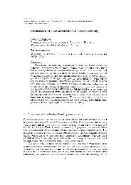
Measurements of the CO-to-H 2 Conversion Factor and Dust-to-Gas ...
Measurements of the CO-to-H 2 Conversion Factor and Dust-to-Gas ...
Measurements of the CO-to-H 2 Conversion Factor and Dust-to-Gas ...

Create successful ePaper yourself
Turn your PDF publications into a flip-book with our unique Google optimized e-Paper software.
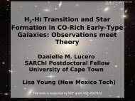
<strong>Measurements</strong> <strong>of</strong> <strong>the</strong><br />
<strong>CO</strong>-<strong>to</strong>-H2 <strong>Conversion</strong> Fac<strong>to</strong>r <strong>and</strong><br />
<strong>Dust</strong>-<strong>to</strong>-<strong>Gas</strong> Ratio in Nearby Galaxies<br />
Karin S<strong>and</strong>strom (MPIA)<br />
Collabora<strong>to</strong>rs: Adam Leroy, Fabian Walter,<br />
KINGFISH team, HERACLES team<br />
Galactic Scale Star Formation<br />
Heidelberg - August 1, 2012
Measuring <strong>the</strong> <strong>CO</strong>-<strong>to</strong>-H2 <strong>Conversion</strong> Fac<strong>to</strong>r.<br />
ΣH2 = α<strong>CO</strong> I<strong>CO</strong><br />
α<strong>CO</strong> = 4.35 M⊙ pc -2 (K km s -1 ) -1<br />
X<strong>CO</strong> = 2×10 20 cm -2 (K km s -1 ) -1<br />
note: α<strong>CO</strong> defined here for<br />
unresolved clouds, includes He<br />
To measure α<strong>CO</strong>:<br />
1. observe <strong>CO</strong><br />
2. use ano<strong>the</strong>r tracer <strong>to</strong> get<br />
<strong>to</strong>tal amount <strong>of</strong> molecular gas<br />
3. compare with observed <strong>CO</strong><br />
O<strong>the</strong>r ways <strong>to</strong> trace <strong>the</strong> <strong>to</strong>tal amount <strong>of</strong> molecular gas:<br />
Dynamics<br />
(i.e. virial masses)<br />
γ-rays<br />
Modeling Line<br />
Emission<br />
<strong>Dust</strong>
O<strong>the</strong>r ways <strong>to</strong> trace <strong>the</strong> <strong>to</strong>tal amount <strong>of</strong> molecular gas:<br />
Dynamics<br />
(i.e. virial masses)<br />
γ-rays<br />
Modeling Line<br />
Emission<br />
<strong>Dust</strong><br />
100.0<br />
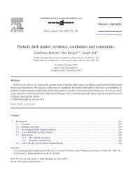
Bolat<strong>to</strong> et al. 2008<br />
Necessary assumptions:<br />
molecular cloud is virialized,<br />
no <strong>CO</strong>-free layer <strong>of</strong> H2<br />
Need <strong>to</strong> resolve GMCs.<br />
Hard <strong>to</strong> do outside <strong>the</strong> Local Group.<br />
Mvir/M<strong>CO</strong><br />
10.0<br />
1.0<br />
Milky Way<br />
Previous results find little<br />
variation away from<br />
MW α<strong>CO</strong>~4.35<br />
7.8 8.0 8.2 8.4 8.6 8.8 9.0<br />
12 + log(O/H)<br />
GMCs in center <strong>of</strong> NGC 6946<br />
have α<strong>CO</strong> ~ α<strong>CO</strong>,MW/2<br />
(Donovan Meyer et al. 2012)
O<strong>the</strong>r ways <strong>to</strong> trace <strong>the</strong> <strong>to</strong>tal amount <strong>of</strong> molecular gas:<br />
Dynamics<br />
(i.e. virial masses)<br />
γ-rays<br />
Modeling Line<br />
Emission<br />
<strong>Dust</strong><br />
Letter <strong>to</strong> <strong>the</strong> Edi<strong>to</strong>r<br />
L48<br />
Necessary assumptions:<br />
distribution <strong>of</strong> cosmic rays<br />
Need <strong>to</strong> observe γ-rays.<br />
Hard <strong>to</strong> do outside <strong>the</strong> Local Group.<br />
Measure MW disk α<strong>CO</strong>~4.35,<br />
MW center α<strong>CO</strong> 5× lower.<br />
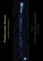
Fig. 1. CR source density as function <strong>of</strong> Galac<strong>to</strong>centric radius R.<br />
Dotted: as used in Strong et al. (2000), solid line: based on pulsars<br />
(Lorimer 2004) as used in this work, vertical bars: SNR data points<br />
from Case & Bhattacharya (1998). Distributions are normalized at<br />
R = 8.5kpc.<br />
A. W. Strong et al.: Distribution <strong>of</strong> cosmic ray sources in <strong>the</strong> Galaxy<br />
X<strong>CO</strong> (cm -2 /(K km s -1 ))<br />
10.0<br />
1.0<br />
MW X<strong>CO</strong> radial gradient from γ-rays<br />
Strong et al. 2004<br />
0.1<br />
0 5 10 15<br />
Radius (kpc)<br />
Fig. 2. X <strong>CO</strong> as function <strong>of</strong> R. Dottedhorizontalline,black:asusedin<br />
Strong & Mat<strong>to</strong>x (1996); Strong et al. (2000); solid line, black: as used<br />
for γ-rays in this work; dashed, dark blue: from Sodroski et al. (1995);<br />
dash-dot, red: using metallicity gradient as described in <strong>the</strong> text, X <strong>CO</strong> ∝<br />
Z −2.5 (Israel 2000), two lines for [O/H] = 0.04 <strong>and</strong> 0.07 dex/kpc; dashdot-dot,light<br />
blue: using X <strong>CO</strong> ∝ Z −1.0 (Boselli et al. 2002) <strong>and</strong> [O/H] =
O<strong>the</strong>r ways <strong>to</strong> trace <strong>the</strong> <strong>to</strong>tal amount <strong>of</strong> molecular gas:<br />
Dynamics<br />
(i.e. virial masses)<br />
γ-rays<br />
Modeling Line<br />
Emission<br />
<strong>Dust</strong><br />
Necessary assumptions:<br />
number <strong>of</strong> different gas<br />
components, velocity/density<br />
structure <strong>of</strong> cloud, etc.<br />
Need <strong>to</strong> observe multiple<br />
molecular gas lines.<br />
Measure galaxy center<br />
α<strong>CO</strong> 5-10× lower than MW.<br />
(e.g. Israel 2009a,b)
O<strong>the</strong>r ways <strong>to</strong> trace <strong>the</strong> <strong>to</strong>tal amount <strong>of</strong> molecular gas:<br />
Dynamics<br />
(i.e. virial masses)<br />
γ-rays<br />
Modeling Line<br />
Emission<br />
<strong>Dust</strong><br />
The Astrophysical Journal, 737:12(13pp),2011August10<br />
Leroy et al.<br />
α<strong>CO</strong><br />
Leroy et al 2011<br />
Necessary assumptions:<br />
dust & gas are well mixed,<br />
DGR & emissivity don’t change<br />
with a<strong>to</strong>mic/molecular phase<br />
Need <strong>to</strong> observe dust mass<br />
tracer (typically far-IR + SED<br />
modeling).<br />
12 + log(O/H)<br />
Widely applied with various<br />
techniques...<br />
Figure 6. Left: α <strong>CO</strong> as a function <strong>of</strong> metallicity. The gray region shows <strong>the</strong> range <strong>of</strong> commonly used α <strong>CO</strong> for <strong>the</strong> Milky Way <strong>and</strong> <strong>the</strong> dashed line indicates <strong>the</strong> value<br />
argued for by Draine et al. (2007) studyingintegratedpho<strong>to</strong>metry<strong>of</strong>SINGSgalaxies.Right:<strong>the</strong>gas-<strong>to</strong>-dustratioδ GDR as a function <strong>of</strong> <strong>the</strong> same metallicities. The<br />
dashed line indicates a linear scaling.
Measuring <strong>the</strong> <strong>Conversion</strong> Fac<strong>to</strong>r with <strong>Dust</strong>.<br />
DGR = ΣD/(ΣHI +α<strong>CO</strong>I<strong>CO</strong>)<br />
unknown<br />
observable<br />
• Fix DGR based on some model or expected DGR.<br />
• Fix DGR based on nearby HI-only line-<strong>of</strong>-sight.<br />
• Solve for both DGR & α <strong>CO</strong> using spatially resolved<br />
measurements.
Measuring <strong>the</strong> <strong>Conversion</strong> Fac<strong>to</strong>r with <strong>Dust</strong>.<br />
DGR = ΣD/(ΣHI +α<strong>CO</strong>I<strong>CO</strong>)<br />
unknown<br />
observable<br />
• Fix DGR based on some model or expected DGR.<br />
• Fix DGR based on nearby HI-only line-<strong>of</strong>-sight.<br />
• Solve for both DGR & α <strong>CO</strong> using spatially resolved<br />
measurements.<br />
Assumption: DGR constant on kpc scales.
Our Technique:<br />
Minimizing Scatter in DGR on kpc scales<br />
car<strong>to</strong>on <strong>of</strong> what happens <strong>to</strong> DGR<br />
when α<strong>CO</strong> is adjusted<br />
DGR =<br />
Σdust<br />
ΣHI +α<strong>CO</strong>I<strong>CO</strong><br />
assume DGR & Xco<br />
constant in this region<br />
I<strong>CO</strong>/ΣHI<br />
• both <strong>CO</strong> <strong>and</strong> H I are detected<br />
Need good S/N maps <strong>of</strong> <strong>CO</strong> & HI.<br />
• a range <strong>of</strong> I<strong>CO</strong>/ΣHI values are present<br />
Need many resolution elements.<br />
• region is small, ok <strong>to</strong> assume DGR & Xco ~ constant<br />
Must select small chunk <strong>of</strong> galaxy, so need high resolution.
Example <strong>of</strong> <strong>the</strong> Technique
Example <strong>of</strong> <strong>the</strong> Technique
1. Measure <strong>CO</strong>, HI & dust<br />
at each point in region.<br />
2. Measure scatter in<br />
DGR at various α<strong>CO</strong>.<br />
3. Find minimum<br />
in scatter.<br />
4. Minimum scatter<br />
=<br />
most “uniform”<br />
DGR in region<br />
=<br />
best-fit α<strong>CO</strong> & DGR
The Observations<br />
DGR = ΣD/(ΣHI +α<strong>CO</strong>I<strong>CO</strong>)<br />
KINGFISH<br />
Key Insights in<strong>to</strong> Nearby Galaxies:<br />
A Far-IR Survey with Herschel<br />
70-500 µm imaging & spectroscopy <strong>of</strong> 62<br />
nearby galaxies with Herschel<br />
Kennicutt et al. 2011<br />
3.6 - 24 µm from SINGS <strong>and</strong> LVL.<br />
(Kennicutt et al. 2003, Dale et al. 2009)<br />
To get ΣD: SED modeling from 3.6 - 350 µm (Aniano+ 2012)<br />
(preserves SPIRE 350 µm’s 25” resolution while<br />
still covering <strong>the</strong> peak <strong>of</strong> <strong>the</strong> dust SED)
The Observations<br />
DGR = ΣD/(ΣHI +α<strong>CO</strong>I<strong>CO</strong>)<br />
THINGS<br />
The HI Nearby Galaxies Survey<br />
HI survey <strong>of</strong> 34 nearby galaxies with <strong>the</strong> VLA<br />
Walter et al. (2008)<br />
Resolution <strong>of</strong> ~12”<br />
HI column density determined<br />
directly from 21cm line.
The Observations<br />
DGR = ΣD/(ΣHI +α<strong>CO</strong>I<strong>CO</strong>)<br />
HERACLES<br />
HERA <strong>CO</strong>-Line Emission Survey<br />
<strong>CO</strong> J=(2-1) survey <strong>of</strong> 48 nearby galaxies with<br />
HERA on <strong>the</strong> IRAM 30m.<br />
Leroy et al. (2009)<br />
Resolution <strong>of</strong> ~13”<br />
Assume (2-1)/(1-0) = 0.7 average for HERACLES sample<br />
(Rosolowsky et al., in prep)
NGC0628 Results
NGC0628 Results
NGC0628 Results
NGC3938 Results
NGC3938 Results
NGC3938 Results
NGC6946 Results
NGC6946 Results
NGC6946 Results
Variations we see in α<strong>CO</strong><br />
• MW α <strong>CO</strong>, no trend with radius.<br />
• Flat MW α <strong>CO</strong> pr<strong>of</strong>ile + central unresolved<br />
dip.<br />
• Overall gradient in α <strong>CO</strong> with radius.<br />
• Low α <strong>CO</strong> everywhere, no clear radial trend.<br />
illustrated with a few examples <strong>of</strong><br />
~face-on, highly resolved galaxies
NGC 4254<br />
0.2 dex<br />
radial pr<strong>of</strong>iles from Schruba+ 2011
NGC 0628<br />
0.2 dex<br />
radial pr<strong>of</strong>iles from Schruba+ 2011
NGC 3184<br />
0.2 dex<br />
radial pr<strong>of</strong>iles from Schruba+ 2011
Variations we see in α<strong>CO</strong><br />
• MW α <strong>CO</strong>, no trend with radius.<br />
• Flat MW α <strong>CO</strong> pr<strong>of</strong>ile + central unresolved<br />
dip.<br />
• Overall gradient in α <strong>CO</strong> with radius.<br />
• Low α <strong>CO</strong> everywhere, no clear radial trend.<br />
illustrated with a few examples <strong>of</strong><br />
~face-on, highly resolved galaxies
NGC 4321<br />
0.2 dex<br />
radial pr<strong>of</strong>iles from Schruba+ 2011<br />
(d)
NGC 4321<br />
0.2 dex<br />
radial pr<strong>of</strong>iles from Schruba+ 2011<br />
(d)
NGC 3351<br />
0.2 dex<br />
radial pr<strong>of</strong>iles from Schruba+ 2011
NGC 3351<br />
0.2 dex<br />
radial pr<strong>of</strong>iles from Schruba+ 2011
Variations we see in α<strong>CO</strong><br />
• MW α <strong>CO</strong>, no trend with radius.<br />
• Flat MW α <strong>CO</strong> pr<strong>of</strong>ile + central unresolved<br />
dip.<br />
• Overall gradient in α <strong>CO</strong> with radius.<br />
• Low α <strong>CO</strong> everywhere, no clear radial trend.<br />
illustrated with a few examples <strong>of</strong><br />
~face-on, highly resolved galaxies
NGC 6946<br />
0.2 dex<br />
radial pr<strong>of</strong>iles from Schruba+ 2011
NGC 6946<br />
0.2 dex<br />
radial pr<strong>of</strong>iles from Schruba+ 2011
Variations we see in α<strong>CO</strong><br />
• MW α <strong>CO</strong>, no trend with radius.<br />
• Flat MW α <strong>CO</strong> pr<strong>of</strong>ile + central unresolved<br />
dip.<br />
• Overall gradient in α <strong>CO</strong> with radius.<br />
• Low α <strong>CO</strong> everywhere, no clear radial trend.<br />
illustrated with a few examples <strong>of</strong><br />
~face-on, highly resolved galaxies
NGC 3627<br />
0.2 dex<br />
al Journal, 142:37(25pp),2011August<br />
radial pr<strong>of</strong>iles from Schruba+ 2011
What drives variations in α<strong>CO</strong>?<br />
NGC 0628<br />
Metallicity?<br />
Large metallicity<br />
gradient.<br />
NGC 6946<br />
Small metallicity<br />
gradient.<br />
~ an order-<strong>of</strong>-magnitude lower than MW disk!
α<strong>CO</strong> & Metallicity<br />
uniform metallicity selection<br />
from Moustakas et al. 2010<br />
strong-line metallicities with<br />
Pilyugin & Thuan 2005 calibration<br />
measurements from HII region spectra<br />
galaxies r<strong>and</strong>omly<br />
assigned <strong>to</strong> panels<br />
NGC 6946<br />
General trend for higher<br />
α<strong>CO</strong> at low Z.<br />
but...<br />
significant scatter in α<strong>CO</strong><br />
at given Z.
<strong>Dust</strong>-<strong>to</strong>-<strong>Gas</strong> Ratio<br />
Linear trend with Z.<br />
Less than a fac<strong>to</strong>r<br />
<strong>of</strong> 2 scatter.<br />
fac<strong>to</strong>r<br />
<strong>of</strong> 2<br />
Constant fraction <strong>of</strong><br />
metals locked up in<br />
dust.
Metallicity isn’t everything...<br />
Is this what we expect?<br />
- dust shielding controls C+/C/<strong>CO</strong> transition<br />
- in MW only 30-50% <strong>of</strong> gas H2 not in <strong>CO</strong> layer<br />
(Fermi Collab. 2010, Planck Collab. 2011)<br />
HI, C+ H 2<br />
<strong>CO</strong><br />
<strong>CO</strong>-free envelope<br />
Z ⊙◉☉⨀<br />
decreasing metallicity DGR<br />
e.g. Maloney & Black 1988, Bolat<strong>to</strong> et al. 1999,<br />
Wolfire et al. 2010, Glover & Mac Low 2011
Metallicity isn’t everything...<br />
Is this what we expect?<br />
- dust shielding controls C+/C/<strong>CO</strong> transition<br />
- in MW only 30-50% <strong>of</strong> gas H2 not in <strong>CO</strong> layer<br />
(Fermi Collab. 2010, Planck Collab. 2011)<br />
HI, C+ H 2<br />
<strong>CO</strong><br />
<strong>CO</strong>-free envelope<br />
Z > Z ⊙◉☉⨀<br />
potential 30%<br />
change in α<strong>CO</strong><br />
Z ⊙◉☉⨀<br />
decreasing metallicity DGR<br />
e.g. Maloney & Black 1988, Bolat<strong>to</strong> et al. 1999,<br />
Wolfire et al. 2010, Glover & Mac Low 2011
What drives variations in α<strong>CO</strong>?
What drives variations in α<strong>CO</strong>?<br />
α<strong>CO</strong> ∝ Σ✳ -0.5
Azimuthal Variations in NGC 6946<br />
Lower α<strong>CO</strong> along <strong>the</strong> spiral arms.
Azimuthal Variations in NGC 6946<br />
Lower α<strong>CO</strong> along <strong>the</strong> spiral arms.
Disagreement with Virial Mass α<strong>CO</strong><br />
<strong>Measurements</strong> in <strong>the</strong> centers<br />
4 Galaxies with virial<br />
mass based α<strong>CO</strong><br />
Virial masses give ~MW or<br />
higher α<strong>CO</strong> in centers <strong>of</strong><br />
2976, 4736 <strong>and</strong> 6946.
Disagreement with Virial Mass α<strong>CO</strong><br />
<strong>Measurements</strong> in <strong>the</strong> centers<br />
4 Galaxies with virial<br />
mass based α<strong>CO</strong><br />
Virial masses give ~MW or<br />
higher α<strong>CO</strong> in centers <strong>of</strong><br />
2976, 4736 <strong>and</strong> 6946.<br />
Several galaxies with<br />
muti-line modeling α<strong>CO</strong><br />
Modeling suggests low α<strong>CO</strong> in<br />
some galaxy centers<br />
NGC 6946 5-10 times lower<br />
than MW - Israel & Baas 2001, Walsh<br />
et al. 2002, Meier & Turner 2004
Our conversion fac<strong>to</strong>rs makes some galaxy centers<br />
have high star-formation efficiency.<br />
Depletion Time:<br />
τDEP = 1/SFE = ΣH2/ΣSFR<br />
Log(τDEP/)<br />
Log(ΣH2)<br />
AGN<br />
SF<br />
higher SFE<br />
compared <strong>to</strong><br />
average<br />
Leroy et al. 2012b, submitted
Summary<br />
• α <strong>CO</strong> can vary by fac<strong>to</strong>r <strong>of</strong> 10 in nearby galaxies -<br />
especially low in <strong>the</strong>ir centers.<br />
• Metallicity not a key driver <strong>of</strong> α <strong>CO</strong> at Z~Z ⊙◉☉⨀ <strong>and</strong> above.<br />
Expected if main effect is <strong>to</strong> change dust shielding <strong>and</strong><br />
alter “<strong>CO</strong>-dark” gas layer.<br />
• Low measured α <strong>CO</strong> enhances SFE in some galaxy centers<br />
over predictions with fixed converison fac<strong>to</strong>r.<br />
• Temperature & velocity dispersion <strong>of</strong> molecular gas are<br />
probably crucial drivers <strong>of</strong> α<strong>CO</strong>.