Spectrum of Ï electrons in bilayer graphene nanoribbons and ...
Spectrum of Ï electrons in bilayer graphene nanoribbons and ...
Spectrum of Ï electrons in bilayer graphene nanoribbons and ...

You also want an ePaper? Increase the reach of your titles
YUMPU automatically turns print PDFs into web optimized ePapers that Google loves.
PHYSICAL REVIEW B 83, 035403 (2011)<br />
<strong>Spectrum</strong> <strong>of</strong> π <strong>electrons</strong> <strong>in</strong> <strong>bilayer</strong> <strong>graphene</strong> <strong>nanoribbons</strong> <strong>and</strong> nanotubes: An analytical approach<br />
J. Ruseckas * <strong>and</strong> G. Juzeliūnas<br />
Institute <strong>of</strong> Theoretical Physics <strong>and</strong> Astronomy, Vilnius University, LT-01108 Vilnius, Lithuania<br />
I. V. Zozoulenko<br />
Solid State Electronics, ITN, L<strong>in</strong>köp<strong>in</strong>g University, SE-601 74 Norköp<strong>in</strong>g, Sweden<br />
(Received 8 October 2010; published 10 January 2011)<br />
We present an analytical description <strong>of</strong> π <strong>electrons</strong> <strong>of</strong> a f<strong>in</strong>ite-size <strong>bilayer</strong> <strong>graphene</strong> with<strong>in</strong> a framework <strong>of</strong><br />
the tight-b<strong>in</strong>d<strong>in</strong>g model. The <strong>bilayer</strong>ed structures considered here are characterized by a rectangular geometry<br />
<strong>and</strong> have a f<strong>in</strong>ite size <strong>in</strong> one or both directions with armchair- <strong>and</strong> zigzag-shaped edges. We provide an exact<br />
analytical description <strong>of</strong> the spectrum <strong>of</strong> π<strong>electrons</strong> <strong>in</strong> the zigzag <strong>and</strong> armchair <strong>bilayer</strong> <strong>graphene</strong> <strong>nanoribbons</strong><br />
<strong>and</strong> nanotubes. We analyze the dispersion relations, the density <strong>of</strong> states, <strong>and</strong> the conductance quantization.<br />
DOI: 10.1103/PhysRevB.83.035403<br />
PACS number(s): 73.22.Pr<br />
I. INTRODUCTION<br />
S<strong>in</strong>ce its isolation <strong>in</strong> 2004, <strong>graphene</strong>—a s<strong>in</strong>gle sheet <strong>of</strong><br />
carbon atoms arranged <strong>in</strong> a honeycomb lattice—has attracted<br />
enormous attention because <strong>of</strong> its highly unusual electronic<br />
<strong>and</strong> transport properties, which are strik<strong>in</strong>gly different from<br />
those <strong>of</strong> conventional semiconductor-based two-dimensional<br />
electronic systems (for a review see Refs. 1–4). The significance<br />
<strong>and</strong> potential impact <strong>of</strong> this new material for electronics<br />
was immediately realized. So far, it has been demonstrated that<br />
<strong>graphene</strong> has the highest carrier mobility at room temperature<br />
<strong>of</strong> any known material. 5 However, <strong>graphene</strong> is a semimetal<br />
with no gap <strong>and</strong> zero density <strong>of</strong> states at the Fermi energy.<br />
This makes it difficult to utilize it <strong>in</strong> electronic devices such<br />
as field-effect transistor (FET) requir<strong>in</strong>g a large on/<strong>of</strong>f current<br />
ratio. The energy gap can be opened <strong>in</strong> a <strong>bilayer</strong> <strong>graphene</strong> by<br />
apply<strong>in</strong>g a gate voltage between the layers. 6 This gate-<strong>in</strong>duced<br />
b<strong>and</strong>gap was demonstrated by Oost<strong>in</strong>ga et al., 7 <strong>and</strong> the on/<strong>of</strong>f<br />
current ratio <strong>of</strong> around 100 at room temperature for a dual-gate<br />
<strong>bilayer</strong> <strong>graphene</strong> FET was reported by IBM. 8<br />
Another way to <strong>in</strong>troduce the gap is to form <strong>graphene</strong> <strong>in</strong>to<br />
<strong>nanoribbons</strong>. 9,10 The conductance <strong>of</strong> <strong>graphene</strong> <strong>nanoribbons</strong><br />
(GNRs) with lithographically etched edges <strong>in</strong>deed revealed<br />
the gap <strong>in</strong> the transport measurements. 11,12 This gap has<br />
been subsequently understood as the edge-disorder-<strong>in</strong>duced<br />
transport gap 13–15 rather than the <strong>in</strong>tr<strong>in</strong>sic energy gap expected<br />
<strong>in</strong> ideal GNRs due to the conf<strong>in</strong>ement 9 or electron <strong>in</strong>teractions<br />
<strong>and</strong> edge effects. 10 In the last few years great progress has<br />
been made <strong>in</strong> fabrication <strong>and</strong> pattern<strong>in</strong>g <strong>of</strong> GNRs with ultrasmooth<br />
<strong>and</strong>/or atomically controlled edges. This <strong>in</strong>cludes, e.g.,<br />
controlled formation <strong>of</strong> edges by Joule heat<strong>in</strong>g, 16 unzipp<strong>in</strong>g<br />
carbon nanotubes to form <strong>nanoribbons</strong>, 17,18 a chemical route to<br />
produce <strong>nanoribbons</strong> with ultrasmooth edges, 19 <strong>and</strong> atomically<br />
precise bottom-up fabrication <strong>of</strong> GNRs. 20 All these advances<br />
<strong>in</strong> <strong>nanoribbons</strong> fabrication will hopefully soon allow electronic<br />
measurements <strong>in</strong> near-perfect <strong>nanoribbons</strong> free from edge or<br />
bulk disorder defects.<br />
An important <strong>in</strong>sight <strong>in</strong>to the electronic properties <strong>of</strong><br />
<strong>graphene</strong> <strong>and</strong> GNRs can be obta<strong>in</strong>ed from exact analytical<br />
approaches. Analytic calculations for the electronic structure<br />
<strong>of</strong> GNRs have been reported <strong>in</strong> Refs. 21–25. The electronic<br />
structure <strong>of</strong> <strong>bilayer</strong> <strong>graphene</strong> was addressed <strong>in</strong> Refs. 26–30,<br />
where the analytical results were presented (both exact <strong>and</strong><br />
perturbative). We are not, however, aware <strong>of</strong> any analytical<br />
treatment <strong>of</strong> <strong>bilayer</strong> GNRs. (Note that a numerical study <strong>of</strong><br />
the magnetob<strong>and</strong> structure <strong>of</strong> GNRs was reported <strong>in</strong> Refs. 31<br />
<strong>and</strong> 32, <strong>and</strong> the analytical <strong>and</strong> numerical treatment <strong>of</strong> the edge<br />
states <strong>in</strong> bi- <strong>and</strong> N-layer <strong>graphene</strong> <strong>and</strong> GNRs was presented <strong>in</strong><br />
Refs. 30 <strong>and</strong> 33). The purpose <strong>of</strong> the present study is to provide<br />
an exact analytical description <strong>of</strong> the spectrum <strong>of</strong> π <strong>electrons</strong><br />
<strong>in</strong> zigzag <strong>and</strong> armchair <strong>bilayer</strong> <strong>nanoribbons</strong> <strong>and</strong> nanotubes,<br />
<strong>in</strong>clud<strong>in</strong>g the dispersion relations, the density <strong>of</strong> states, <strong>and</strong><br />
the conductance quantization.<br />
The paper is organized as follows: In order to illustrate<br />
our method, <strong>in</strong> Sec. II we present known analytical results<br />
for a simpler system, monolayer <strong>graphene</strong> <strong>of</strong> a f<strong>in</strong>ite size.<br />
Subsequently <strong>in</strong> Sec. III we derive the ma<strong>in</strong> analytical<br />
expressions for the energy spectrum <strong>of</strong> f<strong>in</strong>ite-size structures<br />
<strong>of</strong> <strong>bilayer</strong> <strong>graphene</strong>. These expressions are used <strong>in</strong> Sec. IV<br />
to analyze the energy spectrum <strong>of</strong> various <strong>bilayer</strong> <strong>graphene</strong><br />
structures near the Fermi energy. F<strong>in</strong>ally, Sec. V summarizes<br />
our f<strong>in</strong>d<strong>in</strong>gs.<br />
II. SINGLE LAYER GRAPHENE<br />
Analytical expressions for the π electron spectrum <strong>in</strong><br />
GNRs <strong>and</strong> <strong>graphene</strong> nanotubes (GNTs), based on tight-b<strong>in</strong>d<strong>in</strong>g<br />
model, were provided <strong>in</strong> Ref. 24. In this section we will<br />
rederive the same expressions <strong>in</strong> an analytically simpler way.<br />
Our method more clearly shows the connection between<br />
solutions for the <strong>in</strong>f<strong>in</strong>ite sheet <strong>of</strong> <strong>graphene</strong> <strong>and</strong> for the<br />
f<strong>in</strong>ite-size sheet. In addition, this simpler method will allow<br />
us to derive later on analytical expressions <strong>of</strong> the π electron<br />
spectrum for more complex systems, <strong>bilayer</strong> GNRs <strong>and</strong> GNTs.<br />
A. Electron spectrum <strong>in</strong> <strong>in</strong>f<strong>in</strong>ite sheet <strong>of</strong> <strong>graphene</strong><br />
First we will consider the π-electron spectrum <strong>in</strong> an <strong>in</strong>f<strong>in</strong>ite<br />
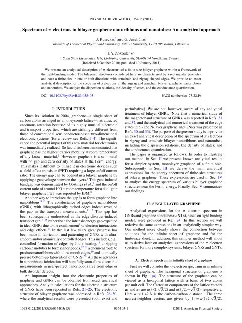
sheet <strong>of</strong> <strong>graphene</strong>. The hexagonal structure <strong>of</strong> <strong>graphene</strong> is<br />
shown <strong>in</strong> Fig. 1(a). The structure <strong>of</strong> the <strong>graphene</strong> can be<br />
viewed as a hexagonal lattice with a basis <strong>of</strong> two atoms<br />
per unit cell. The Cartesian components <strong>of</strong> the lattice vectors<br />
a 1 <strong>and</strong> a 2 are a(3/2, √ 3/2) <strong>and</strong> a(3/2,− √ 3/2), respectively.<br />
Here a ≈ 1.42 Å is the carbon-carbon distance. 1 The three<br />
nearest-neighbor vectors are given by δ 1 = a(1/2, √ 3/2),<br />
1098-0121/2011/83(3)/035403(13) 035403-1<br />
©2011 American Physical Society
J. RUSECKAS, G. JUZELIŪNAS, AND I. V. ZOZOULENKO PHYSICAL REVIEW B 83, 035403 (2011)<br />
(a) (b) (c)<br />
FIG. 1. (Color onl<strong>in</strong>e) (a) Honeycomb lattice structure <strong>of</strong> <strong>graphene</strong>, made out <strong>of</strong> two <strong>in</strong>terpenetrat<strong>in</strong>g triangular lattices; a 1 <strong>and</strong> a 2 are the<br />
lattice unit vectors, <strong>and</strong> δ i , i = 1,2,3, are the nearest-neighbor vectors. (b) Indication <strong>of</strong> labels <strong>of</strong> carbon atoms <strong>in</strong> the rectangular unit cell.<br />
(c) Brillou<strong>in</strong> zones for hexagonal unit cell (solid hexagon) <strong>and</strong> rectangular unit cell (dashed rectangle). The Dirac po<strong>in</strong>ts are <strong>in</strong>dicated by solid<br />
circles for the hexagonal unit cell <strong>and</strong> hollow circles for the rectangular unit cell.<br />
δ 2 = a(1/2,− √ 3/2), <strong>and</strong> δ 1 = a(−1,0). The tight-b<strong>in</strong>d<strong>in</strong>g<br />
Hamiltonian for <strong>electrons</strong> <strong>in</strong> <strong>graphene</strong> has the form<br />
H gr =−t ∑ 〈i,j〉(a † i b j + b † j a i) , (1)<br />
<strong>in</strong>stead <strong>of</strong> the wave vector components k x <strong>and</strong> k y . Then us<strong>in</strong>g<br />
the coord<strong>in</strong>ates <strong>of</strong> the vectors δ j we have<br />
( )<br />
˜φ(k) = e −i κ 3 + 2e<br />
i ξ κ<br />
6 cos (9)<br />
2<br />
where the operators a i <strong>and</strong> b i annihilate an electron on<br />
sublattice A at site R A i<br />
<strong>and</strong> on sublattice B at site R B i ,<br />
respectively. The parameter t is the nearest-neighbor hopp<strong>in</strong>g<br />
energy (t ≈ 2.8 eV). From now on we will write all energies<br />
<strong>in</strong> the units <strong>of</strong> the hopp<strong>in</strong>g <strong>in</strong>tegral t; therefore, we will set<br />
t = 1. Let us label the elementary cells <strong>of</strong> the lattice with two<br />
numbers, p <strong>and</strong> q. Then the atoms <strong>in</strong> the sublattices A <strong>and</strong> B are<br />
positioned at R A p,q = pa 1 + qa 2 <strong>and</strong> R B p,q = δ 1 + pa 1 + qa 2 ,<br />
respectively.<br />
The π-electron wave function satisfies the Schröd<strong>in</strong>ger<br />
equation,<br />
H = E . (2)<br />
We search for the eigenvectors <strong>of</strong> the Hamiltonian [Eq. (1)] <strong>in</strong><br />
the form <strong>of</strong> plane waves (Bloch states) by tak<strong>in</strong>g the probability<br />
amplitudes to f<strong>in</strong>d an atom <strong>in</strong> the sites R A p,q <strong>and</strong> RB p,q <strong>of</strong> the<br />
sublattices A <strong>and</strong> B as<br />
ψ A p,q = cA e ik·RA p,q , ψ<br />
B<br />
p,q = c B e ik·RB p,q . (3)<br />
Thus Eq. (2) yields the follow<strong>in</strong>g eigenvalue equations for the<br />
coefficients c A <strong>and</strong> c B :<br />
where<br />
−Ec A = c B ˜φ(k), (4)<br />
−Ec B = c A ˜φ(−k), (5)<br />
˜φ(k) ≡ e ik·δ 1<br />
+ e ik·δ 2<br />
+ e ik·δ 3<br />
. (6)<br />
From Eqs. (4) <strong>and</strong> (5) we get the eigenenergies <strong>and</strong> the<br />
correspond<strong>in</strong>g coefficients determ<strong>in</strong><strong>in</strong>g the eigenvectors<br />
E(k) = s 1 | ˜φ(k), c A =−˜φ(k)<br />
E(k) , cB = 1, (7)<br />
where s 1 =±1. In anticipation <strong>of</strong> rectangular geometry we<br />
<strong>in</strong>troduce dimensionless Cartesian components <strong>of</strong> the wave<br />
vector<br />
κ = 3ak x , ξ = √ 3ak y (8)<br />
035403-2<br />
<strong>and</strong> the expression for the eigenenergies becomes 1<br />
√<br />
( ) ( )<br />
ξ ξ<br />
( κ<br />
)<br />
E(k) = s 1 1 + 4 cos 2 + 4 cos cos . (10)<br />
2<br />
2 2<br />
To satisfy boundary conditions it is useful to adopt a larger<br />
unit cell characterized by the same geometry as the whole sheet<br />
<strong>of</strong> <strong>graphene</strong>. S<strong>in</strong>ce we are <strong>in</strong>terested <strong>in</strong> configurations <strong>of</strong> the<br />
<strong>graphene</strong> with rectangular geometry, we will use a rectangular<br />
unit cell, as has been done <strong>in</strong> Ref. 24. Such a unit cell has<br />
four atoms labeled with symbols l, λ, ρ, r, shown <strong>in</strong> Fig. 1(b).<br />
The atoms with labels l <strong>and</strong> ρ belong to the sublattice A, <strong>and</strong><br />
the atoms with labels λ <strong>and</strong> r belong to the sublattice B. The<br />
position <strong>of</strong> the unit cell is <strong>in</strong>dicated with two numbers, n <strong>and</strong><br />
m. The first Brillou<strong>in</strong> zone correspond<strong>in</strong>g to the rectangular<br />
unit cell conta<strong>in</strong>s the values <strong>of</strong> the wave vectors κ <strong>and</strong> ξ <strong>in</strong><br />
the <strong>in</strong>tervals −π κ
SPECTRUM OF π ELECTRONS IN BILAYER GRAPHENE ... PHYSICAL REVIEW B 83, 035403 (2011)<br />
E<br />
4<br />
2<br />
0<br />
-2<br />
-4<br />
0 0.5 1 1.5 2 2.5 3<br />
FIG. 2. (Color onl<strong>in</strong>e) Left: dispersion branches <strong>of</strong> <strong>graphene</strong><br />
for rectangular unit cell, calculated accord<strong>in</strong>g to Eq. (16). Right:<br />
dispersion branches for ξ = 0, show<strong>in</strong>g propagat<strong>in</strong>g solutions (red<br />
solid) <strong>and</strong> evanescent solutions (green dashed).<br />
where<br />
c l =−s 3 e −i κ 2<br />
φ(κ,ξ)<br />
E(κ,ξ) , c λ = s 3 e −i 1 2 (κ+ξ) , (14)<br />
φ(κ,ξ) = s 3 e −i κ 2 + 2 cos<br />
( ξ<br />
2<br />
|κ|<br />
)<br />
, (15)<br />
<strong>and</strong> s 3 =±1 <strong>in</strong>dicates the dispersion branches that appear due<br />
to the smaller Brillou<strong>in</strong> zone. The equation for the energy now<br />
becomes<br />
√<br />
( ) ( )<br />
ξ ξ<br />
( κ<br />
)<br />
E(κ,ξ) = s 1 1 + 4 cos 2 + s 3 4 cos cos .<br />
2<br />
2 2<br />
(16)<br />
This equation has been obta<strong>in</strong>ed <strong>in</strong> Ref. 24. Zero-energy po<strong>in</strong>ts<br />
<strong>of</strong> the <strong>graphene</strong> honeycomb lattice with dispersion relation<br />
given by Eq. (10) are at the po<strong>in</strong>ts K = (2π,2π/3) <strong>and</strong> K ′ =<br />
(2π,−2π/3), where coord<strong>in</strong>ates are given <strong>in</strong> (κ,ξ) space. K<br />
po<strong>in</strong>ts correspond to the corners <strong>of</strong> the first Brillou<strong>in</strong> zone.<br />
Us<strong>in</strong>g the Brillou<strong>in</strong> zone correspond<strong>in</strong>g to the rectangular unit<br />
cell, the zero-energy po<strong>in</strong>ts have coord<strong>in</strong>ates (0,± 2π ) <strong>and</strong> the<br />
3<br />
number <strong>of</strong> these po<strong>in</strong>ts is only two, as shown <strong>in</strong> Fig. 1(c).<br />
S<strong>in</strong>ce we will consider f<strong>in</strong>ite-size <strong>graphene</strong> sheets, evanescent<br />
solutions become important. Solutions exponentially<br />
decreas<strong>in</strong>g or <strong>in</strong>creas<strong>in</strong>g <strong>in</strong> the x direction can be obta<strong>in</strong>ed by<br />
tak<strong>in</strong>g κ = i|κ| <strong>in</strong> Eqs. (13), (14), <strong>and</strong> (16), whereas solutions<br />
exponentially decreas<strong>in</strong>g or <strong>in</strong>creas<strong>in</strong>g <strong>in</strong> the y direction can<br />
be obta<strong>in</strong>ed by tak<strong>in</strong>g ξ = i|ξ|. The dependency <strong>of</strong> the energy<br />
on κ when ξ = 0 is shown <strong>in</strong> Fig. 2. We see that the branches<br />
with real <strong>and</strong> imag<strong>in</strong>ary κ do not <strong>in</strong>tersect at |κ| > 0.<br />
B. Electron spectrum <strong>in</strong> various s<strong>in</strong>gle-layer<br />
<strong>graphene</strong> structures<br />
From the boundary conditions we get restrictions on the<br />
possible values <strong>of</strong> the wave vectors κ,ξ. We will consider<br />
the structures <strong>of</strong> <strong>graphene</strong> that have a set <strong>of</strong> N rectangular<br />
unit cells <strong>in</strong> the x (armchair) direction <strong>and</strong> a set <strong>of</strong> N + 1/2<br />
rectangular unit cells <strong>in</strong> the y (zigzag) direction, so that there<br />
are N hexagons along the y axis. Note that rectangular unit<br />
cell shown <strong>in</strong> Fig. 1(b) extends over the whole hexagon <strong>in</strong> the<br />
y direction, whereas it extends over more that one hexagon <strong>in</strong><br />
the x direction.<br />
Us<strong>in</strong>g the periodic boundary condition, correspond<strong>in</strong>g to<br />
the <strong>graphene</strong> torus, we obta<strong>in</strong> the possible values <strong>of</strong> the wave<br />
vectors κ,ξ as<br />
ξ j = 2π ⌊ ⌋ ⌊ ⌋ ⌊ ⌋<br />
N N N − 1<br />
N j, j =− , − + 1,...,<br />
2 2<br />
2<br />
(17)<br />
κ ν = 2π ⌊ ⌋ ⌊ ⌋ ⌊ ⌋<br />
N N N − 1<br />
N ν, ν =− , − + 1,...,<br />
2 2 2<br />
(18)<br />
Here ⌊·⌋ denotes the <strong>in</strong>teger part <strong>of</strong> a number. Thus the<br />
spectrum <strong>of</strong> a <strong>graphene</strong> torus is given by Eq. (16) replac<strong>in</strong>g κ<br />
<strong>and</strong> ξ by κ ν <strong>and</strong> ξ j .<br />
For <strong>graphene</strong> armchair nanotubes one has the periodic<br />
boundary condition <strong>in</strong> the x direction <strong>and</strong> the requirement<br />
ψ 0,n,r = ψ 0,n,l = ψ N +1,n,l = ψ N +1,n,r = 0forthey direction.<br />
S<strong>in</strong>ce the energy [Eq. (16)] does not depend on the sign <strong>of</strong> wave<br />
vector ξ, we will search for the eigenvectors <strong>of</strong> the Hamiltonian<br />
[Eq. (1)] as a superposition <strong>of</strong> periodic solutions [Eq. (11)] with<br />
ξ <strong>and</strong> −ξ,<br />
ψ m,n,α = ac α (ξ,κ ν )e iξm+iκνn + bc α (−ξ,κ ν )e −iξm+iκνn , (19)<br />
where κ ν is given by Eq. (18) <strong>and</strong> ξ needs to be determ<strong>in</strong>ed.<br />
From the boundary conditions we get a system <strong>of</strong> two equations<br />
for the coefficients a <strong>and</strong> b:<br />
ac r,l (ξ,κ ν ) + bc r,l (−ξ,κ ν ) = 0, (20)<br />
ae iξ(N +1) c r,l (ξ,κ ν ) + be −iξ(N +1) c r,l (−ξ,κ ν ) = 0. (21)<br />
This system <strong>of</strong> equations has nonzero solutions only when the<br />
determ<strong>in</strong>ant is zero. From Eqs. (13) <strong>and</strong> (14) it follows that the<br />
coefficients c r,l (ξ,κ) do not depend on the sign <strong>of</strong> ξ, <strong>and</strong> we<br />
get the condition s<strong>in</strong>[ξ(N + 1)] = 0or<br />
ξ =<br />
πj , j = 1,...,N . (22)<br />
N + 1<br />
Additionally, there are two N-fold degenerate levels correspond<strong>in</strong>g<br />
to ξ = π with energies E =±1. The states <strong>of</strong> those<br />
levels have zero wave function amplitudes at the l <strong>and</strong> r sites.<br />
For <strong>graphene</strong> zigzag nanotubes one has the periodic<br />
boundary condition <strong>in</strong> the y direction <strong>and</strong> the condition<br />
ψ m,0,r = ψ m,N+1,l = 0 for the x direction. Similar to the<br />
armchair nanotubes, the energy [Eq. (16)] does not depend on<br />
the sign <strong>of</strong> wave vector κ, <strong>and</strong> we search for the eigenvectors<br />
<strong>of</strong> the Hamiltonian [Eq. (1)] as a superposition <strong>of</strong> periodic<br />
solutions [Eq. (11)] with κ <strong>and</strong> −κ,<br />
ψ m,n,α = ac α (ξ j ,κ)e iξ j m+iκn + bc α (ξ j ,−κ)e iξ j m−iκn , (23)<br />
where ξ j is given by Eq. (17) <strong>and</strong> κ needs to be determ<strong>in</strong>ed.<br />
From the boundary conditions we get a system <strong>of</strong> two equations<br />
for the coefficients a <strong>and</strong> b:<br />
ac r (ξ j ,κ) + bc r (ξ j ,−κ) = 0, (24)<br />
ac l (ξ j ,κ)e iκ(N+1) + bc l (ξ j ,−κ)e −iκ(N+1) = 0. (25)<br />
Us<strong>in</strong>g Eqs. (13) <strong>and</strong> (14) we f<strong>in</strong>d that nonzero solutions are<br />
possible when<br />
( )<br />
s<strong>in</strong>(κN)<br />
s<strong>in</strong> [ κ ( ξj<br />
N + 1 )] =−s 3 2 cos . (26)<br />
2<br />
2<br />
035403-3
J. RUSECKAS, G. JUZELIŪNAS, AND I. V. ZOZOULENKO PHYSICAL REVIEW B 83, 035403 (2011)<br />
The possible values <strong>of</strong> wave vector κ should obey this equation.<br />
The same condition has been obta<strong>in</strong>ed <strong>in</strong> Ref. 24. Equation<br />
(26) allows for the imag<strong>in</strong>ary values <strong>of</strong> wave vector κ. The<br />
imag<strong>in</strong>ary values appear when ξ c < |ξ j |
SPECTRUM OF π ELECTRONS IN BILAYER GRAPHENE ... PHYSICAL REVIEW B 83, 035403 (2011)<br />
(a)<br />
(b)<br />
(c)<br />
(d)<br />
FIG. 3. (Color onl<strong>in</strong>e) Upper part:<br />
sublatices A 1 , A 2 , B 1 ,<strong>and</strong>B 2 on <strong>bilayer</strong><br />
<strong>graphene</strong> <strong>in</strong> AB-α stack<strong>in</strong>g (a) <strong>and</strong> ABβ<br />
stack<strong>in</strong>g (b). Lower part: <strong>in</strong>dication<br />
<strong>of</strong> labels <strong>of</strong> carbon atoms used <strong>in</strong> the<br />
description <strong>of</strong> the π-electron spectrum for<br />
<strong>bilayer</strong> <strong>graphene</strong> with AB-α stack<strong>in</strong>g (c)<br />
<strong>and</strong> AB-β stack<strong>in</strong>g (d).<br />
λ 1 <strong>and</strong> r 1 to sublattice A 1 ,atomsl 2 <strong>and</strong> ρ 2 to sublattice B 2 ,<br />
<strong>and</strong> atoms λ 2 <strong>and</strong> r 2 to sublattice A 2 .<br />
We search for the solutions <strong>of</strong> the form<br />
ψ m,n,αp = c αp e iξm+iκn , (38)<br />
where α = l,ρ,λ,r is the label <strong>of</strong> atoms <strong>and</strong> p = 1,2 isthe<br />
number <strong>of</strong> the layer. For the AB-α stack<strong>in</strong>g, this solution can<br />
be obta<strong>in</strong>ed from Eq. (28) us<strong>in</strong>g the equalities<br />
whereas for the AB-β stack<strong>in</strong>g the coefficients are<br />
c r1 = (c A 1<br />
) ∗ , c ρ1 = (c B 1<br />
) ∗ e −ik·δ 1<br />
,<br />
c λ1 = (c A 1<br />
) ∗ e −ik·a 1<br />
, c l1 = (c B 1<br />
) ∗ e −i2ak x<br />
,<br />
c r2 = (c A 2<br />
) ∗ e −ik·a 2<br />
, c ρ2 = (c B 2<br />
) ∗ e −iak x<br />
,<br />
c λ2 = (c A 2<br />
) ∗ , c l2 = (c B 2<br />
) ∗ e ik·δ 1<br />
.<br />
(41)<br />
(42)<br />
c r1 = c B 1<br />
, c ρ1 = c A 1<br />
e −ik·δ 1<br />
,<br />
c λ1 = c B 1<br />
e −ik·a 1<br />
, c l1 = c A 1<br />
e −i2ak x<br />
,<br />
c r2 = c B 2<br />
e −iak x<br />
, c ρ2 = c A 2<br />
e −ik·δ 1<br />
,<br />
c λ2 = c B 2<br />
e ik·δ 2<br />
, c l2 = c A 2<br />
e iak x<br />
,<br />
(39)<br />
(40)<br />
As was the case for monolayer <strong>graphene</strong>, to take <strong>in</strong>to<br />
account the smaller Brillou<strong>in</strong> zone we need two dispersion<br />
branches: one with κ <strong>and</strong> one with 2π + κ. Us<strong>in</strong>gEq.(34) or<br />
Eq. (36) we obta<strong>in</strong> the coefficients <strong>of</strong> the eigenvectors. The<br />
expressions for the coefficients are presented <strong>in</strong> Appendix A.<br />
The expression for the energy becomes<br />
E(κ,ξ) = s 1<br />
√<br />
γ 2<br />
2 + V 2 +|φ(κ,ξ)| 2 + s 2<br />
√<br />
γ<br />
4<br />
4 +|φ(κ,ξ)|2 (4V 2 + γ 2 ), (43)<br />
which reduces to<br />
( √ )<br />
γ γ<br />
E(κ,ξ) = s 1 s 2<br />
2 + 2<br />
4 +|φ(κ,ξ)|2<br />
for V = 0. Here<br />
|φ(κ,ξ)| 2 = 1 + 4 cos 2 ( ξ<br />
2<br />
(44)<br />
) ( ) ξ<br />
( κ<br />
)<br />
+ s 3 4 cos cos , (45)<br />
2 2<br />
<strong>and</strong> s 3 =±1 <strong>in</strong>dicates the dispersion branches that appear due<br />
to the smaller Brillou<strong>in</strong> zone.<br />
In addition to the propagat<strong>in</strong>g waves, for f<strong>in</strong>ite-size <strong>bilayer</strong><br />
<strong>graphene</strong> sheets evanescent solutions become important. Solutions<br />
exponentially decreas<strong>in</strong>g or <strong>in</strong>creas<strong>in</strong>g <strong>in</strong> the x direction<br />
can be obta<strong>in</strong>ed by tak<strong>in</strong>g κ = i|κ|. Solutions exponentially<br />
decreas<strong>in</strong>g or <strong>in</strong>creas<strong>in</strong>g <strong>in</strong> the y direction can be obta<strong>in</strong>ed by<br />
tak<strong>in</strong>g ξ = i|ξ|. In addition to the purely imag<strong>in</strong>ary ξ there are<br />
solutions, correspond<strong>in</strong>g to s 3 =−1, hav<strong>in</strong>g complex values<br />
<strong>of</strong> ξ. The dependency <strong>of</strong> the energy on the wave vector κ when<br />
the wave vector ξ is constant <strong>and</strong> on the wave vector ξ when<br />
the wave vector κ is constant is shown <strong>in</strong> Fig. 4. We see that<br />
now, <strong>in</strong> contrast to the <strong>graphene</strong> monolayer, the branches with<br />
real <strong>and</strong> imag<strong>in</strong>ary κ can have the same energy.<br />
035403-5
J. RUSECKAS, G. JUZELIŪNAS, AND I. V. ZOZOULENKO PHYSICAL REVIEW B 83, 035403 (2011)<br />
E<br />
4<br />
2<br />
0<br />
-2<br />
-4<br />
0 0.5 1 1.5 2 2.5 3<br />
|κ|<br />
E<br />
4<br />
2<br />
0<br />
-2<br />
-4<br />
0 0.5 1 1.5 2 2.5 3<br />
Re ξ+Im ξ<br />
FIG. 4. (Color onl<strong>in</strong>e) Dispersion branches <strong>of</strong> <strong>bilayer</strong> <strong>graphene</strong>:<br />
dependency <strong>of</strong> the energy on the wave vector κ when the wave<br />
vector ξ is constant (ξ = 0) (left) <strong>and</strong> on the wave vector ξ when the<br />
wave vector κ is constant (κ = 1.0) (right). Propagat<strong>in</strong>g solutions are<br />
shown with red solid l<strong>in</strong>e, evanescent solutions with green dashed<br />
l<strong>in</strong>e, <strong>and</strong> evanescent oscillat<strong>in</strong>g solutions with complex value <strong>of</strong><br />
the wave vector ξ are shown with blue dotted l<strong>in</strong>e. In order to show<br />
the structure <strong>of</strong> the dispersion branches more clearly, the value <strong>of</strong> the<br />
parameter γ is set sufficiently large, γ = 0.5.<br />
B. Electron spectrum <strong>in</strong> various <strong>bilayer</strong> <strong>graphene</strong> structures<br />
We will consider the structures <strong>of</strong> <strong>bilayer</strong> <strong>graphene</strong> that have<br />
a set <strong>of</strong> N rectangular unit cells <strong>in</strong> the x (armchair) direction<br />
<strong>and</strong> a set <strong>of</strong> N + 1/2 rectangular unit cells <strong>in</strong> the y (zigzag)<br />
direction, so that there are N hexagons along the y axis. Note<br />
that the rectangular unit cells shown <strong>in</strong> Figs. 3(c) <strong>and</strong> 3(d)<br />
extend over the whole hexagon <strong>in</strong> the y direction, whereas<br />
they extend over more that one hexagon <strong>in</strong> the x direction.<br />
In pr<strong>in</strong>ciple, <strong>in</strong> the case <strong>of</strong> <strong>bilayer</strong> <strong>graphene</strong> nanotubes the<br />
numbers N or N for the <strong>in</strong>ner <strong>and</strong> outer cyl<strong>in</strong>ders are different.<br />
However, for simplicity we will consider them to be the same,<br />
which is a good approximation for sufficiently large tubes<br />
when N →∞or N →∞.<br />
As we found for the <strong>graphene</strong> monolayer, from the<br />
boundary conditions we get restrictions on the possible values<br />
<strong>of</strong> the wave vectors κ <strong>and</strong> ξ. Us<strong>in</strong>g a periodic boundary<br />
condition correspond<strong>in</strong>g to the <strong>bilayer</strong> <strong>graphene</strong> torus, we f<strong>in</strong>d<br />
that the possible values <strong>of</strong> the wave vectors κ <strong>and</strong> ξ are given<br />
by Eqs. (17) <strong>and</strong> (18).<br />
For <strong>bilayer</strong> <strong>graphene</strong> armchair nanotubes one has the<br />
periodic boundary condition for the x direction <strong>and</strong> the<br />
condition<br />
ψ 0,n,rp = ψ 0,n,lp = ψ N +1,n,lp = ψ N +1,n,rp = 0 (46)<br />
for the y direction. Here p = 1,2 is the number <strong>of</strong> the<br />
layer. This condition is the same for both the AB-α <strong>and</strong><br />
AB-β stack<strong>in</strong>gs. For <strong>bilayer</strong> <strong>graphene</strong> with AB-α stack<strong>in</strong>g<br />
the coefficients c rp ,l p<br />
(ξ,κ) do not depend on the sign <strong>of</strong> ξ <strong>and</strong><br />
we get the same conditions [Eqs. (18) <strong>and</strong> (22)] for the wave<br />
vectors κ <strong>and</strong> ξ as we got for the monolayer <strong>graphene</strong> armchair<br />
tubes.<br />
For <strong>bilayer</strong> <strong>graphene</strong> with AB-β stack<strong>in</strong>g the coefficients<br />
c rp ,l p<br />
(ξ,κ) depend on the sign <strong>of</strong> ξ, <strong>and</strong> condition for the<br />
possible values <strong>of</strong> the wave vector ξ is much more complicated.<br />
There are eight boundary conditions <strong>in</strong> the y direction. In<br />
<strong>bilayer</strong> <strong>graphene</strong> there are four eigenstates with different wave<br />
vectors along the y direction, ξ (1) , ξ (2) , ξ (3) , <strong>and</strong> ξ (4) ,hav<strong>in</strong>gthe<br />
same energy: E(κ,ξ (1) ) = E(κ,ξ (2) ) = E(κ,ξ (3) ) = E(κ,ξ (4) ),<br />
as is evident from Fig. 4. Two or four <strong>of</strong> the wave vectors ξ (1) ,<br />
ξ (2) , ξ (3) , <strong>and</strong> ξ (4) can be imag<strong>in</strong>ary or complex numbers. S<strong>in</strong>ce<br />
the energy does not depend on the sign <strong>of</strong> ξ, we can form a wave<br />
function from superposition <strong>of</strong> eight waves. From the boundary<br />
conditions [Eq. (46)], the result<strong>in</strong>g set <strong>of</strong> l<strong>in</strong>ear equations<br />
can have nonzero solutions only if the 8 × 8 determ<strong>in</strong>ant is<br />
zero. The analytical form <strong>of</strong> this condition is too large <strong>and</strong> too<br />
complicated to be useful.<br />
For <strong>bilayer</strong> <strong>graphene</strong> zigzag nanotubes one has the periodic<br />
boundary condition for the y direction <strong>and</strong> the condition<br />
ψ m,0,r1 = ψ m,N+1,l1 = ψ m,0,l2 = ψ m,N+1,r2 = 0 (47)<br />
for the x direction. Here p = 1,2 is the number <strong>of</strong> the layer.<br />
This condition is the same for both the AB-α <strong>and</strong> AB-β<br />
stack<strong>in</strong>gs. In the <strong>bilayer</strong> <strong>graphene</strong> there are two eigenstates<br />
with wave vectors along the x direction, κ (1) <strong>and</strong> κ (2) ,hav<strong>in</strong>g<br />
different absolute values but correspond<strong>in</strong>g to the same energy:<br />
E(κ (1) ,ξ) = E(κ (2) ,ξ). One or both <strong>of</strong> the wave vectors κ (1)<br />
<strong>and</strong> κ (2) can be imag<strong>in</strong>ary. The energy can be equal only if the<br />
signs s 1 , s 2 obey the condition<br />
s (2)<br />
1 s(2) 2<br />
=−s (1)<br />
1 s(1) 2<br />
(48)<br />
When the bias potential is zero, V = 0, from the equality <strong>of</strong><br />
the energy we can express κ (2) as<br />
( κ<br />
s (2)<br />
(2)<br />
) ( κ<br />
3<br />
cos = s (1)<br />
(1)<br />
)<br />
3<br />
cos<br />
2<br />
2<br />
+ s (1) γ<br />
1 s(1) 2<br />
2 cos ( )E(κ (1) ,ξ). (49)<br />
ξ<br />
2<br />
When V ≠ 0,<br />
)<br />
)<br />
s (2)<br />
3<br />
cos<br />
( κ<br />
(2)<br />
2<br />
= s (1)<br />
3<br />
cos<br />
( κ<br />
(1)<br />
γ<br />
±<br />
2 cos ( ) √ 4E<br />
ξ<br />
2 V 2 + γ 2 (E 2 − V 2 ).<br />
2<br />
(50)<br />
There are four boundary conditions <strong>in</strong> the x direction. S<strong>in</strong>ce the<br />
energy does not depend on the sign <strong>of</strong> κ, we can form a wave<br />
function from superposition <strong>of</strong> four waves. From the boundary<br />
conditions [Eq. (47)] the result<strong>in</strong>g set <strong>of</strong> l<strong>in</strong>ear equations can<br />
have nonzero solutions only if the 4 × 4 determ<strong>in</strong>ant is zero.<br />
The possible values <strong>of</strong> the wave vector ξ are given by Eq. (17),<br />
<strong>and</strong> the conditions for the possible values <strong>of</strong> the wave vector<br />
κ are given <strong>in</strong> Appendix B.<br />
For an N × N sheet <strong>of</strong> <strong>bilayer</strong> <strong>graphene</strong>, open boundary<br />
conditions <strong>in</strong> the y direction are the same as for armchair<br />
nanotubes, Eq. (46), <strong>and</strong> <strong>in</strong> the x direction are the same as for<br />
zigzag nanotubes, Eq. (47). For AB-α stack<strong>in</strong>g, the conditions<br />
for the possible values <strong>of</strong> the wave vectors κ <strong>and</strong> ξ are a<br />
comb<strong>in</strong>ation <strong>of</strong> the conditions for zigzag <strong>and</strong> armchair <strong>bilayer</strong><br />
<strong>graphene</strong> tubes. Specifically, when V = 0, the conditions are<br />
given by Eqs. (22) <strong>and</strong> (B1) or (B2). When V ≠ 0, the<br />
conditions are given by Eqs. (22) <strong>and</strong> (B3). For AB-β stack<strong>in</strong>g<br />
it is impossible to separate conditions for the wave vector<br />
ξ from the conditions for the wave vector κ. The result<strong>in</strong>g<br />
expressions are very large <strong>and</strong> complicated.<br />
C. Summary <strong>of</strong> the possible values <strong>of</strong> wave vectors<br />
For structures <strong>of</strong> <strong>bilayer</strong> <strong>graphene</strong>, the energy spectrum is<br />
completely determ<strong>in</strong>ed by Eqs. (44) or(43) with appropriate<br />
expressions for wave vectors κ <strong>and</strong> ξ.<br />
2<br />
035403-6
SPECTRUM OF π ELECTRONS IN BILAYER GRAPHENE ... PHYSICAL REVIEW B 83, 035403 (2011)<br />
Equations presented <strong>in</strong> Appendix B make one quantum<br />
number dependent on the other. This dependence appears<br />
because <strong>of</strong> zigzag-shaped edges. For structures where zigzag<br />
edges do not exist or their effect can be disregarded, the wave<br />
vector κ ν can be replaced by a cont<strong>in</strong>uous variable.<br />
Thus, the possible values <strong>of</strong> wave vectors for various<br />
structures are as follows:<br />
1. For the armchair <strong>bilayer</strong> <strong>graphene</strong> ribbon <strong>of</strong> <strong>in</strong>f<strong>in</strong>ite<br />
length with AB-α stack<strong>in</strong>g, the wave vectors are determ<strong>in</strong>ed<br />
by<br />
0 κ π, ξ j = πj , j = 1,...,N . (51)<br />
N + 1<br />
2. For the armchair <strong>bilayer</strong> <strong>graphene</strong> ribbon <strong>of</strong> <strong>in</strong>f<strong>in</strong>ite<br />
length with AB-β stak<strong>in</strong>g we have 0 κ π <strong>and</strong> the equation<br />
for the possible values <strong>of</strong> ξ is complicated.<br />
3. For the zigzag <strong>bilayer</strong> <strong>graphene</strong> ribbon <strong>of</strong> <strong>in</strong>f<strong>in</strong>ite length<br />
we have 0 ξ π, <strong>and</strong> the conditions for the possible values<br />
<strong>of</strong> κ, given <strong>in</strong> Appendix B, are different for AB-α <strong>and</strong> AB-β<br />
stack<strong>in</strong>gs.<br />
4. For the zigzag <strong>bilayer</strong> carbon tube <strong>of</strong> <strong>in</strong>f<strong>in</strong>ite length with<br />
AB-α or AB-β stack<strong>in</strong>g, the wave vectors are determ<strong>in</strong>ed by<br />
0 κ π, ξ j = 2π N j, ⌊ ⌋ ⌊ ⌋ ⌊ ⌋ (52)<br />
N N N − 1<br />
j =− , − + 1,..., .<br />
2 2<br />
2<br />
5. For the armchair <strong>bilayer</strong> carbon tube <strong>of</strong> <strong>in</strong>f<strong>in</strong>ite length<br />
with AB-αor AB-β stack<strong>in</strong>g,<br />
κ ν = 2π ⌊ N<br />
N ν, ν =− 2<br />
⌊ N − 1<br />
⌊ ⌋ N<br />
− + 1,...,<br />
2<br />
2<br />
⌋<br />
,<br />
⌋<br />
, 0 ξ π.<br />
(53)<br />
Tak<strong>in</strong>g <strong>in</strong>to account the ranges <strong>of</strong> the possible values <strong>of</strong> the<br />
wave vectors, zero-energy po<strong>in</strong>ts for various structures with<br />
bias potential V = 0 are as follows:<br />
6. For zigzag <strong>bilayer</strong> carbon tube, zero-energy po<strong>in</strong>ts are<br />
(0, 2π 3 ), (0,− 2π 3 ).<br />
7. For armchair <strong>bilayer</strong> carbon tube, zero-energy po<strong>in</strong>t is<br />
(0, 2π 3 ).<br />
8. The dispersion <strong>of</strong> armchair <strong>bilayer</strong> <strong>graphene</strong> ribbon has<br />
only one zero-energy po<strong>in</strong>t (0, 2π 3 ).<br />
9. For zigzag <strong>bilayer</strong> <strong>graphene</strong> ribbon dispersion, this po<strong>in</strong>t<br />
cannot be shown <strong>in</strong> the real plane.<br />
IV. BAND STRUCTURE NEAR THE FERMI ENERGY<br />
In this Section we focus on only the part <strong>of</strong> the spectrum<br />
with the smallest absolute value <strong>of</strong> energy. This part corresponds<br />
to s 2 =−1, s 3 =−1. In order to obta<strong>in</strong> an approximate<br />
expression for the energy spectrum near the Fermi energy we<br />
exp<strong>and</strong> Eq. (45) <strong>in</strong> a power series near the zero po<strong>in</strong>t κ = 0,<br />
ξ = 2π/3, yield<strong>in</strong>g<br />
[ (<br />
|φ(κ,ξ)| 2 ≈ 3 √ )<br />
κ 2<br />
( 3<br />
1 −<br />
4 3 2 q + q 2 1 + q ) ]<br />
2 √ 3<br />
[<br />
≈ 3 κ 2 ( ) 2<br />
]<br />
4 3 + q −<br />
κ2<br />
4 √ . (54)<br />
3<br />
Here q ≡ ξ − 2π/3 <strong>and</strong> |κ| ≪1, |q| ≪1. Substitut<strong>in</strong>g<br />
Eq. (54) <strong>in</strong>to Eq. (44)orEq.(43) one obta<strong>in</strong>s the approximate<br />
expression for the energy spectrum. Thus, when the bias<br />
potential is zero, V = 0, the approximate expression for the<br />
energy is<br />
E(κ,ξ) = s 1<br />
⎧<br />
⎨<br />
⎩ −γ 2 + √ √√√<br />
γ 2<br />
4 + 3 4<br />
[<br />
κ 2<br />
3 + (<br />
q −<br />
) ] ⎫ 2 ⎬<br />
κ2<br />
4 √ 3 ⎭<br />
(55)<br />
Furthermore, assum<strong>in</strong>g that |φ(κ,ξ)| 2 ≪ γ , the branch <strong>of</strong><br />
Eq. (44) with s 2 =−1, s 3 =−1 takes the form<br />
|φ(κ,ξ)| 2<br />
E(κ,ξ) ≈ s 1 . (56)<br />
γ<br />
When V ≠ 0 <strong>and</strong> V ≪ γ ,thenEq.(43) becomes<br />
2V<br />
|φ(κ,ξ)| 4<br />
E(κ,ξ) ≈ s 1 V − s 1<br />
γ 2 |φ(κ,ξ)|2 + s 1 . (57)<br />
2Vγ 2<br />
The <strong>bilayer</strong> <strong>graphene</strong> has a gap at |φ(κ,ξ)| 2 = 2V 2 . However,<br />
s<strong>in</strong>ce the parameter γ is small, γ ≪ 1, the approximate<br />
expressions <strong>of</strong> Eqs. (56) <strong>and</strong> (57) are suitable only for very<br />
small values <strong>of</strong> |κ| <strong>and</strong> |q|.<br />
The spectrum <strong>of</strong> various structures <strong>of</strong> <strong>bilayer</strong> <strong>graphene</strong> can<br />
be obta<strong>in</strong>ed from the approximate expressions for |φ(κ,ξ)| 2<br />
near zero po<strong>in</strong>ts. In contrast to Eqs. (56) √ <strong>and</strong> (57), the energy<br />
<strong>of</strong> monolayer <strong>graphene</strong> is E(κ,ξ) = s 1 |φ(κ,ξ)|2 . Thus, the<br />
analysis <strong>of</strong> the square root <strong>of</strong> |φ(κ,ξ)| 2 essentially was done<br />
<strong>in</strong> Ref. 24. Go<strong>in</strong>g back to the orig<strong>in</strong>al wave vectors k x <strong>and</strong> k y ,<br />
the b<strong>and</strong> structure <strong>of</strong> <strong>bilayer</strong> <strong>graphene</strong> tubes <strong>and</strong> ribbons when<br />
V = 0as<strong>in</strong>Ref.24 can be summarized by the equation<br />
(<br />
E ν (k ‖ ) ≈ s 1 − γ √ )<br />
γ<br />
2 + 2<br />
4 + 9 4 a2 [(k ‖ − ¯k<br />
‖ σ )2 + k⊥ν σ 2]<br />
,<br />
(58)<br />
where k ‖ <strong>and</strong> k ⊥ν denote the longitud<strong>in</strong>al (cont<strong>in</strong>uous) <strong>and</strong><br />
the transverse (quantized) components <strong>of</strong> the wave vector,<br />
respectively. Index σ specifies the structure. Further <strong>in</strong> this<br />
Section we will consider only the case when V = 0.<br />
A. Quantum conductance<br />
With<strong>in</strong> the framework <strong>of</strong> the L<strong>and</strong>auer approach, 34–37 the<br />
zero-temperature conductance <strong>of</strong> an ideal wire is equal to<br />
G(E) = 2e2<br />
h<br />
∑<br />
g ν T ν (E), (59)<br />
where 2e 2 /h is conductance quantum, g ν is the b<strong>and</strong> degeneracy,<br />
<strong>and</strong> transmission coefficient T ν is 0 or 1 depend<strong>in</strong>g on<br />
ν<br />
035403-7
J. RUSECKAS, G. JUZELIŪNAS, AND I. V. ZOZOULENKO PHYSICAL REVIEW B 83, 035403 (2011)<br />
σ<br />
TABLE I. Degeneracy g σ ν <strong>of</strong> the νth b<strong>and</strong> energy |Eσ ν (k ‖ = 0)|<br />
Armchair <strong>bilayer</strong> carbon tube 1(ν = 0), 2(ν ≠ 0)<br />
Zigzag <strong>bilayer</strong> carbon tube 2<br />
Armchair <strong>bilayer</strong> <strong>graphene</strong> ribbon 1<br />
Zigzag <strong>bilayer</strong> <strong>graphene</strong> ribbon 1<br />
whether the νth b<strong>and</strong> is open or closed for charge carriers with<br />
energy E.<br />
When bias potential is zero, V = 0, the transmission<br />
coefficient is T ν (E) = (E − Eν σ ) for conduction b<strong>and</strong>s <strong>and</strong><br />
T ν (E) = (|E − Eν σ |) for valence b<strong>and</strong>s. Here Eσ ν are the<br />
subb<strong>and</strong> threshold energies <strong>and</strong> (x) is the Heaviside step<br />
function. When the approximation Eq. (58) is valid, the<br />
subb<strong>and</strong> threshold energies are<br />
(<br />
)<br />
E σ ν = s 1<br />
− γ 2 + √<br />
γ<br />
2<br />
4 + 9 4 a2 k σ 2<br />
⊥ν<br />
g σ ν<br />
. (60)<br />
The degeneracies are shown <strong>in</strong> Table I. The values <strong>of</strong> g ν<br />
for armchair <strong>bilayer</strong> carbon tube <strong>and</strong> zigzag <strong>bilayer</strong> <strong>graphene</strong><br />
ribbon with ν>1, represented <strong>in</strong> Table I, should be doubled,<br />
because electron or hole states with ±k ‖ ≠ 0 are degenerate.<br />
The electron or hole conductance <strong>of</strong> armchair <strong>and</strong> zigzag<br />
<strong>bilayer</strong> carbon tubes <strong>and</strong> their parent <strong>graphene</strong> ribbons has thus<br />
the form <strong>of</strong> a ladder, symmetrically ascend<strong>in</strong>g with the <strong>in</strong>crease<br />
<strong>in</strong> energy for <strong>electrons</strong>, <strong>and</strong> with the decrease <strong>of</strong> energy for<br />
holes. For the charge carrier energy that falls between the nth<br />
<strong>and</strong> (n + 1)th b<strong>and</strong>s, the wire conductance equals<br />
⎧<br />
n armchair <strong>bilayer</strong> ribbon,<br />
⎪⎨<br />
G(E) = 2e2 2n + 2 zigzag <strong>bilayer</strong> ribbon,<br />
(61)<br />
h ⎪⎩ 2n zigzag <strong>bilayer</strong> carbon tube,<br />
2(2n + 1) armchair <strong>bilayer</strong> carbon tube.<br />
The conductance for <strong>bilayer</strong> <strong>graphene</strong> ribbons has been<br />
numerically calculated <strong>in</strong> Ref. 31. Equation (61) for the<br />
conductance co<strong>in</strong>cides with that <strong>of</strong> Ref. 31.<br />
B. Density <strong>of</strong> states<br />
The density <strong>of</strong> states (DOS) <strong>of</strong> a quantum wire, <strong>in</strong>clud<strong>in</strong>g<br />
a factor 2 for the sp<strong>in</strong> degeneracy, reads<br />
ρ(E) = 2 ∑<br />
[ ] dEν (k ‖ ,k ⊥ν ) −1<br />
. (62)<br />
π dk ‖<br />
ν<br />
The summation <strong>in</strong>cludes all transverse modes with energy<br />
E ν E. Us<strong>in</strong>g Eq. (58) we obta<strong>in</strong> the DOS <strong>of</strong> <strong>bilayer</strong><br />
<strong>graphene</strong>,<br />
ρ(E) = 2<br />
3πa<br />
∑<br />
ν<br />
g ν<br />
(2|E|+γ )<br />
√ (|E|− ∣ ∣E σ ν<br />
∣ ∣<br />
)(<br />
|E|+<br />
∣ ∣E σ ν<br />
∣ ∣ + γ<br />
)<br />
× ( |E|− ∣ ∣ E<br />
σ<br />
ν<br />
∣ ∣<br />
)<br />
. (63)<br />
The <strong>in</strong>dex ν is ν = 0,±1,±2,... for <strong>bilayer</strong> <strong>graphene</strong> tubes<br />
<strong>and</strong> armchair <strong>bilayer</strong> <strong>graphene</strong> ribbons, <strong>and</strong> ν = 0,1,2,...for<br />
zigzag <strong>bilayer</strong> <strong>graphene</strong> ribbons. The electron density at zero<br />
temperature is obta<strong>in</strong>ed by the <strong>in</strong>tegration <strong>of</strong> the DOS from<br />
the charge neutrality po<strong>in</strong>t μ 0 = 0 to the Fermi energy,<br />
n =<br />
∫ EF<br />
0<br />
ρ(E)dE. (64)<br />
Us<strong>in</strong>g Eq. (63) we get<br />
n σ (E F ) = 4 ∑ √ (|EF<br />
g ν |− ∣ ∣) E<br />
σ 3πa<br />
ν (|EF |+ ∣ ∣ E<br />
σ ν + γ )<br />
ν<br />
×(|E F |−|E ν |). (65)<br />
C. Armchair <strong>bilayer</strong> carbon tube<br />
For the armchair <strong>bilayer</strong> carbon tube we have that κ <strong>in</strong><br />
Eq. (54) has discrete values κ ν = 2πν/N, ν = 0,±1,..., <strong>and</strong><br />
q is cont<strong>in</strong>uous. Thus the energy spectrum has the form<br />
E ν (k y )<br />
{ √<br />
= s 1 − γ 2 + γ 2<br />
4 + 9 [<br />
4 a2 (k y − ¯k y,ν ) 2 + 4π ] } 2 ν 2<br />
,<br />
9a 2 N 2<br />
with<br />
(66)<br />
¯k y,ν =<br />
2π<br />
3 √ 3a + π 2 ν 2<br />
3aN . (67)<br />
2<br />
Conduction (valence) b<strong>and</strong> bottoms (tops) are equal to<br />
(<br />
E ν = s 1 − γ √ )<br />
γ<br />
2 + 2<br />
4 + π 2 ν 2<br />
. (68)<br />
N 2<br />
The distance between the m<strong>in</strong>ima <strong>of</strong> the dispersion branches<br />
with the <strong>in</strong>dices s 2 =−1 <strong>and</strong> s 2 =+1isγ . The number ν<br />
<strong>of</strong> subb<strong>and</strong>s with the <strong>in</strong>dex s 2 =−1 <strong>and</strong> energy smaller than<br />
the energies <strong>of</strong> the subb<strong>and</strong>s with <strong>in</strong>dex s 2 =+1 is greater<br />
than 1 only when the number <strong>of</strong> rectangular unit cells <strong>in</strong> the x<br />
direction, N, is sufficiently large. Us<strong>in</strong>g the equation E ν,max =<br />
γ <strong>and</strong> estimat<strong>in</strong>g the subb<strong>and</strong> threshold energy [Eq. (68)] as<br />
E ν ≈ π 2 ν 2 /(γN 2 ), one obta<strong>in</strong>s that the requirement ν ≫ 1<br />
leads to N ≫ π/γ. In calculations we used N = 100.<br />
The b<strong>and</strong> structure, calculated with exact Eqs. (44) <strong>and</strong><br />
(45) <strong>and</strong> approximated accord<strong>in</strong>g to Eq. (66), is represented <strong>in</strong><br />
Fig. 5. One sees that Eq. (66) provides a good approximation<br />
<strong>of</strong> the exact results. Also shown is the DOS, calculated<br />
with Eqs. (63) <strong>and</strong> (68), <strong>and</strong> the conductance G(E) =<br />
(2e 2 /h)2(2n + 1).<br />
0.3<br />
0.2<br />
E<br />
0.1<br />
0.0<br />
1.0 1.1 1.2 1.3 1.4<br />
ak y<br />
25<br />
20<br />
15<br />
ρ<br />
10<br />
5<br />
0.00 0.04 0.08 0.12<br />
E<br />
25<br />
20<br />
G<br />
15<br />
10<br />
5<br />
0<br />
0.00 0.04 0.08 0.12<br />
E<br />
FIG. 5. (Color onl<strong>in</strong>e) B<strong>and</strong> structure <strong>of</strong> armchair <strong>bilayer</strong> carbon<br />
tubes (left), DOS (center), <strong>and</strong> conductance (right). The number <strong>of</strong><br />
rectangular unit cells <strong>in</strong> the x direction N = 100. Solid red l<strong>in</strong>es<br />
are calculated accord<strong>in</strong>g to Eqs. (44) <strong>and</strong>(45); dashed green l<strong>in</strong>es<br />
represent the approximation <strong>of</strong> Eq. (66). B<strong>and</strong>s with s 2 =+1 are not<br />
shown. DOS is given <strong>in</strong> units <strong>of</strong> a −1 <strong>and</strong> is calculated accord<strong>in</strong>g to<br />
Eqs. (63)<strong>and</strong>(68). The conductance is given <strong>in</strong> units <strong>of</strong> 2e 2 /h<strong>and</strong> is<br />
calculated us<strong>in</strong>g Eq. (61).<br />
035403-8
SPECTRUM OF π ELECTRONS IN BILAYER GRAPHENE ... PHYSICAL REVIEW B 83, 035403 (2011)<br />
D. Zigzag <strong>bilayer</strong> carbon tube<br />
Dist<strong>in</strong>ct from armchair <strong>bilayer</strong> carbon tubes, which are<br />
always metallic when V = 0, zigzag <strong>bilayer</strong> carbon tube has<br />
a gapless spectrum if j ∗ ≡ N /3 is an <strong>in</strong>teger, E j=j ∗(κ =<br />
0) = 0. Otherwise, the zigzag <strong>bilayer</strong> carbon tube spectrum<br />
has a gap. If N /3 is not an <strong>in</strong>teger, the b<strong>and</strong> <strong>in</strong>dex <strong>of</strong><br />
the lowest conduction (highest valence) b<strong>and</strong> can be equal<br />
either to j ∗ ≡ (N − 1)/3 ortoj ∗ ≡ (N + 1)/3. As a result<br />
<strong>of</strong> expansion near zero-energy po<strong>in</strong>ts <strong>in</strong> powers <strong>of</strong> κ <strong>and</strong><br />
2π(j − j ∗ )/N ,wearriveat<br />
|φ(κ,ξ)| 2 ≈ 3 ) (q ν 2 4<br />
+ κ2<br />
, (69)<br />
3<br />
where<br />
⎧<br />
2π<br />
⎪⎨ N ∣ ν − 1 3∣ ≪ 1 , semiconduct<strong>in</strong>g,<br />
q ν = (<br />
2π|ν|<br />
⎪⎩ 1 + πν )<br />
N 2 √ ≪ 1, metallic,<br />
3N<br />
with ν = 0,±1,....The wave vector component κ is cont<strong>in</strong>uous.<br />
The energy spectrum has the form<br />
[ √<br />
E ν (k x ) = s 1 − γ 2 + γ 2<br />
4 + 9 ( ) ]<br />
4 a2 kx 2 + q2 ν<br />
. (70)<br />
3a 2<br />
Conduction (valence) b<strong>and</strong> bottoms (tops) are equal to<br />
(<br />
E ν = s 1 − γ √ )<br />
γ<br />
2 + 2<br />
4 + 3 4 q2 ν . (71)<br />
The number ν <strong>of</strong> subb<strong>and</strong>s with the <strong>in</strong>dex s 2 =−1 <strong>and</strong> energy<br />
smaller than the energies <strong>of</strong> the subb<strong>and</strong>s with <strong>in</strong>dex s 2 =+1<br />
is greater than 1 only when the number <strong>of</strong> hexagons <strong>in</strong> the y<br />
direction N is sufficiently large. Approximat<strong>in</strong>g Eq. (71) as<br />
3π 2 ν 2 /(γ N 2 ) we get N ≫ √ 3π/γ. In calculations we used<br />
N = 102 for metallic tubes <strong>and</strong> N = 100 for semiconduct<strong>in</strong>g<br />
tubes.<br />
The b<strong>and</strong> structure, calculated us<strong>in</strong>g exact Eqs. (44) <strong>and</strong><br />
(45) <strong>and</strong> approximated accord<strong>in</strong>g to Eq. (70) for metallic <strong>and</strong><br />
for semiconduct<strong>in</strong>g tubes is shown <strong>in</strong> Fig. 6. One sees that<br />
Eq. (70) provides a good approximation <strong>of</strong> the exact results.<br />
Also shown is the DOS, calculated with Eqs. (63) <strong>and</strong> (71),<br />
<strong>and</strong> the conductance G(E) = (2e 2 /h)2n.<br />
E. Armchair <strong>bilayer</strong> <strong>graphene</strong> ribbon<br />
For the armchair <strong>bilayer</strong> <strong>graphene</strong> ribbon with AB-α<br />
stack<strong>in</strong>g, the condition for the wave-vector component ξ<br />
has a simple expression. When V = 0 <strong>and</strong> j ∗ ≡ 2(N + 1)/3<br />
is an <strong>in</strong>teger, then the armchair <strong>bilayer</strong> <strong>graphene</strong> ribbon<br />
is metallic. Then <strong>in</strong>dex ν = j − j ∗ = 0 corresponds to the<br />
zero-energy b<strong>and</strong>. If 2(N + 1)/3 is not an <strong>in</strong>teger, the armchair<br />
<strong>bilayer</strong> <strong>graphene</strong> ribbon spectrum has a gap, <strong>and</strong> the b<strong>and</strong><br />
closest to zero is either j ∗ ≡ (2N + 1)/3orj ∗ ≡ (2N + 3)/3,<br />
depend<strong>in</strong>g on which <strong>of</strong> these two numbers is an <strong>in</strong>teger. For<br />
κ,ν/N ≪ 1 we get Eq. (69) with<br />
⎧<br />
π<br />
⎪⎨ N + 1 ∣ ν − 1 3∣ ≪ 1 ,<br />
semiconduct<strong>in</strong>g,<br />
q ν = (<br />
)<br />
π|ν|<br />
πν<br />
⎪⎩ 1 +<br />
N + 1 4 √ ≪ 1 , metallic,<br />
3(N + 1)<br />
(72)<br />
0.15<br />
0.10<br />
E<br />
0.05<br />
0.00<br />
0.00 0.05 0.10<br />
ak x<br />
0.15<br />
E 0.10<br />
0.05<br />
0.00<br />
0.00 0.05 0.10<br />
ak x<br />
20<br />
15<br />
ρ 10<br />
5<br />
0.00 0.04 0.08 0.12<br />
E<br />
20<br />
15<br />
ρ 10<br />
5<br />
0.00 0.04 0.08 0.12<br />
E<br />
15<br />
10<br />
G<br />
5<br />
0.00 0.04 0.08 0.12<br />
E<br />
15<br />
10<br />
G<br />
5<br />
0.00 0.04 0.08 0.12<br />
E<br />
FIG. 6. (Color onl<strong>in</strong>e) Upper part: b<strong>and</strong> structure <strong>of</strong> metallic<br />
zigzag <strong>bilayer</strong> carbon tubes (left), DOS (center) <strong>and</strong> conductance<br />
(right). The number <strong>of</strong> hexagons <strong>in</strong> the y direction N = 102. Lower<br />
part: b<strong>and</strong> structure <strong>of</strong> semiconduct<strong>in</strong>g zigzag <strong>bilayer</strong> carbon tubes<br />
(left), DOS (center) <strong>and</strong> conductance (right). The number <strong>of</strong> hexagons<br />
<strong>in</strong> the y direction N = 100. Solid red l<strong>in</strong>es are calculated accord<strong>in</strong>g<br />
Eqs. (44), (45); dashed green l<strong>in</strong>es represent approximation (70).<br />
B<strong>and</strong>s with s 2 =+1 are not shown. DOS is given <strong>in</strong> units <strong>of</strong> a −1 <strong>and</strong><br />
is calculated accord<strong>in</strong>g to Eqs. (63), (71). The conductance is given<br />
<strong>in</strong> units <strong>of</strong> 2e 2 /h <strong>and</strong> is calculated us<strong>in</strong>g Eq. (61).<br />
with ν = 0,±1,.... The wave vector component κ is cont<strong>in</strong>uous.<br />
The difference between the boundary conditions for<br />
armchair <strong>bilayer</strong> <strong>graphene</strong> ribbons <strong>and</strong> zigzag <strong>bilayer</strong> <strong>graphene</strong><br />
tubes results <strong>in</strong> about two-times smaller b<strong>and</strong> spac<strong>in</strong>g <strong>in</strong> the<br />
armchair ribbon spectrum than was found for the zigzag tube<br />
spectrum.<br />
The energy spectrum has the form<br />
[ √<br />
E ν (k x ) = s 1 − γ 2 + γ 2<br />
4 + 9 ( ) ]<br />
4 a2 kx 2 + q2 ν<br />
. (73)<br />
3a 2<br />
Conduction (valence) b<strong>and</strong> bottoms (tops) are equal to<br />
(<br />
E ν = s 1 − γ √ )<br />
γ<br />
2 + 2<br />
4 + 3 4 q2 ν . (74)<br />
The number ν <strong>of</strong> subb<strong>and</strong>s with the <strong>in</strong>dex s 2 =−1 <strong>and</strong> energy<br />
smaller than the energies <strong>of</strong> the subb<strong>and</strong>s with <strong>in</strong>dex s 2 =+1<br />
is greater than 1 only when the number <strong>of</strong> hexagons <strong>in</strong> the y<br />
direction N is sufficiently large. Approximat<strong>in</strong>g Eq. (74) as<br />
3π 2 ν 2 /4γ (N + 1) 2 we get N ≫ √ 3π/(2γ ). In calculations<br />
we used N = 101 for metallic ribbons <strong>and</strong> N = 100 for<br />
semiconduct<strong>in</strong>g ribbons.<br />
The b<strong>and</strong> structure, calculated with the use <strong>of</strong> exact<br />
Eqs. (44) <strong>and</strong> (45) <strong>and</strong> approximated accord<strong>in</strong>g to Eq. (73)<br />
for metallic <strong>and</strong> semiconduct<strong>in</strong>g ribbons is shown <strong>in</strong> Fig. 7.<br />
One sees that Eq. (73) provides a good approximation <strong>of</strong> the<br />
exact results. Also shown is the DOS, calculated with Eqs. (63)<br />
<strong>and</strong> (74), <strong>and</strong> the conductance G(E) = (2e 2 /h)n.<br />
For the armchair <strong>bilayer</strong> <strong>graphene</strong> ribbon with AB-β<br />
stack<strong>in</strong>g there are no explicit expressions for the possible<br />
values <strong>of</strong> q.<br />
F. Zigzag <strong>bilayer</strong> <strong>graphene</strong> ribbon<br />
In zigzag <strong>bilayer</strong> <strong>graphene</strong> ribbons the wave vector component<br />
q is cont<strong>in</strong>uous while the possible values <strong>of</strong> κ are<br />
given by the solutions <strong>of</strong> Eqs. (49) <strong>and</strong> (B1), plus Eq. (B2)for<br />
AB-α stack<strong>in</strong>g or Eq. (B5) forAB-β stack<strong>in</strong>g, presented <strong>in</strong><br />
035403-9
J. RUSECKAS, G. JUZELIŪNAS, AND I. V. ZOZOULENKO PHYSICAL REVIEW B 83, 035403 (2011)<br />
0.10<br />
E<br />
0.05<br />
0.00<br />
0.00 0.05 0.10<br />
ak x<br />
0.10<br />
E<br />
0.05<br />
0.00<br />
0.00 0.05 0.10<br />
ak x<br />
15<br />
10<br />
ρ<br />
5<br />
0.00 0.04 0.08 0.12<br />
E<br />
15<br />
10<br />
ρ<br />
5<br />
0.00 0.04 0.08 0.12<br />
E<br />
15<br />
10<br />
G<br />
5<br />
0<br />
0.00 0.04 0.08 0.12<br />
E<br />
15<br />
10<br />
G<br />
5<br />
0<br />
0.00 0.04 0.08 0.12<br />
E<br />
FIG. 7. (Color onl<strong>in</strong>e) Upper part: b<strong>and</strong> structure <strong>of</strong> metallic<br />
armchair <strong>bilayer</strong> <strong>graphene</strong> ribbon with AB-α stack<strong>in</strong>g (left), DOS<br />
(center), <strong>and</strong> conductance (right). The number <strong>of</strong> hexagons <strong>in</strong> the y<br />
direction N = 101. Lower part: b<strong>and</strong> structure <strong>of</strong> semiconduct<strong>in</strong>g<br />
armchair <strong>bilayer</strong> <strong>graphene</strong> ribbon with AB-α stack<strong>in</strong>g (left), DOS<br />
(center), <strong>and</strong> conductance (right). The number <strong>of</strong> hexagons <strong>in</strong> the<br />
y direction N = 100. Solid red l<strong>in</strong>es are calculated accord<strong>in</strong>g to<br />
Eqs. (44) <strong>and</strong>(45); dashed green l<strong>in</strong>es represent the approximation<br />
calculated with Eq. (73). B<strong>and</strong>s with s 2 =+1 are not shown. DOS<br />
is given <strong>in</strong> units <strong>of</strong> a −1 <strong>and</strong> is calculated accord<strong>in</strong>g to Eqs. (63) <strong>and</strong><br />
(74). The conductance is given <strong>in</strong> units <strong>of</strong> 2e 2 /h <strong>and</strong> is calculated<br />
us<strong>in</strong>g Eq. (61).<br />
Appendix B. S<strong>in</strong>ce equations for κ depend on the value <strong>of</strong> the<br />
wave vector ξ, <strong>in</strong> zigzag <strong>bilayer</strong> <strong>graphene</strong> ribbons longitud<strong>in</strong>al<br />
<strong>and</strong> transverse motions are not separable. When the energy<br />
<strong>of</strong> the subb<strong>and</strong> with the <strong>in</strong>dex s 2 =−1 is smaller than the<br />
energies <strong>of</strong> the subb<strong>and</strong>s with <strong>in</strong>dex s 2 =+1, only one <strong>of</strong><br />
the wave vectors κ (1) <strong>and</strong> κ (2) has a real value. Therefore, the<br />
energy subb<strong>and</strong>s can be labeled by the value <strong>of</strong> κ (1) ≡ κ ν only.<br />
Depend<strong>in</strong>g on the value <strong>of</strong> |ξ|, wave vectors κ ν with<br />
ν = 0,1 can become imag<strong>in</strong>ary. There are two critical values<br />
ξ c(1) , ξ c(2) (ξ c(1) 2 arccos[N/(2N + 1)]. The imag<strong>in</strong>ary solutions κ ν<br />
represent edge states <strong>in</strong> zigzag <strong>bilayer</strong> <strong>graphene</strong> ribbons.<br />
The energy b<strong>and</strong>s <strong>of</strong> <strong>bilayer</strong> <strong>graphene</strong> are asymmetric near<br />
the po<strong>in</strong>t q = 0. The subb<strong>and</strong>s (except those correspond<strong>in</strong>g to<br />
edge states) can be approximated by tak<strong>in</strong>g κ ν ≈ πν/N <strong>and</strong><br />
the m<strong>in</strong>imum <strong>of</strong> <strong>of</strong> the subb<strong>and</strong> located at ξ c(2) :<br />
with<br />
E ν (k y )<br />
{ √<br />
= s 1 − γ 2 + γ 2<br />
4 + 9 [<br />
4 a2 (k y − ¯k y ) 2 + π ] } 2 ν 2<br />
,<br />
9a 2 N 2<br />
(75)<br />
¯k y = ξ c(2)<br />
√<br />
3a<br />
. (76)<br />
The critical value ξ c(2) <strong>of</strong> the wave vector tends to the limit<br />
2π/3 as the number N grows. Conduction (valence) b<strong>and</strong><br />
0.3<br />
0.2<br />
E<br />
0.1<br />
0.0<br />
1.0 1.1 1.2 1.3 1.4<br />
ak y<br />
15<br />
10<br />
ρ<br />
5<br />
0.00 0.02 0.04 0.06 0.08<br />
E<br />
10<br />
G<br />
5<br />
0.00 0.04 0.08 0.12<br />
E<br />
FIG. 8. (Color onl<strong>in</strong>e) B<strong>and</strong> structure <strong>of</strong> zigzag <strong>bilayer</strong> <strong>graphene</strong><br />
ribbon with AB-α stack<strong>in</strong>g (left), DOS (center), <strong>and</strong> conductance<br />
(right). The number <strong>of</strong> rectangular unit cells <strong>in</strong> the x direction N =<br />
60. Solid red l<strong>in</strong>es are calculated accord<strong>in</strong>g to Eqs. (44)<strong>and</strong>(45), with<br />
the allowed values <strong>of</strong> the wave vector κ obta<strong>in</strong>ed by solv<strong>in</strong>g Eqs. (B1),<br />
(B2), <strong>and</strong> (49); dashed green l<strong>in</strong>es represent the approximation <strong>of</strong><br />
Eq. (75). B<strong>and</strong>s with s 2 =+1 are not shown. DOS is given <strong>in</strong> units<br />
<strong>of</strong> a −1 . The conductance is given <strong>in</strong> units <strong>of</strong> 2e 2 /h <strong>and</strong> is calculated<br />
us<strong>in</strong>g Eq. (61).<br />
bottoms (tops) are equal to<br />
(<br />
E ν = s 1 − γ √ )<br />
γ<br />
2 + 2<br />
4 + π 2 ν 2<br />
. (77)<br />
4N 2<br />
The number ν <strong>of</strong> <strong>of</strong> subb<strong>and</strong>s with the <strong>in</strong>dex s 2 =−1<br />
<strong>and</strong> energy smaller than the energies <strong>of</strong> the subb<strong>and</strong>s with<br />
<strong>in</strong>dex s 2 =+1 is greater than 1 only when the number <strong>of</strong><br />
rectangular unit cells <strong>in</strong> the x direction, N, is sufficiently large.<br />
Approximat<strong>in</strong>g Eq. (77)asπ 2 ν 2 /(4γN 2 ) we get N ≫ π/(2γ ).<br />
In calculations we used N = 60.<br />
The b<strong>and</strong> structure for zigzag <strong>bilayer</strong> <strong>graphene</strong> ribbons<br />
with AB-α stack<strong>in</strong>g, calculated us<strong>in</strong>g exact Eqs. (44) <strong>and</strong> (45)<br />
with the allowed values <strong>of</strong> the wave vector κ obta<strong>in</strong>ed by<br />
solv<strong>in</strong>g Eqs. (B1), (B2), <strong>and</strong> (49), as well as the approximation<br />
<strong>of</strong> Eq. (75), are represented <strong>in</strong> Fig. 8. Also shown is the<br />
DOS <strong>and</strong> the conductance G(E) = (2e 2 /h)(2n + 2). The DOS<br />
is calculated from the exact b<strong>and</strong> structure <strong>and</strong> also us<strong>in</strong>g<br />
Eqs. (63) <strong>and</strong> (74), tak<strong>in</strong>g the threshold energies for ν = 0,1to<br />
be E ν=0,1 = 0. The b<strong>and</strong> structure <strong>of</strong> zigzag <strong>bilayer</strong> <strong>graphene</strong><br />
ribbons with AB-β stack<strong>in</strong>g is very similar to the b<strong>and</strong><br />
structure <strong>of</strong> ribbons with AB-α stack<strong>in</strong>g, only the critical<br />
values ξ c(1) , ξ c(2) are slightly different.<br />
Tak<strong>in</strong>g the limit N →∞<strong>in</strong> the zigzag <strong>bilayer</strong> <strong>graphene</strong><br />
ribbon with AB-β stack<strong>in</strong>g one can obta<strong>in</strong> the edge states<br />
<strong>of</strong> Ref. 30. However, care should be taken not to lose any<br />
solutions. For large N we can write the absolute value <strong>of</strong> the<br />
imag<strong>in</strong>ary wave vector i|κ| as |κ| =κ (0) + δ, where κ (0) is the<br />
solution <strong>of</strong> the equation<br />
e − κ(0)<br />
2 = 2 cos(ξ/2), (78)<br />
<strong>and</strong> δ is a small correction. From Eq. (44) it follows that such<br />
a value <strong>of</strong> κ (0) ensures the equality E(iκ (0) ,ξ) = 0. Exp<strong>and</strong><strong>in</strong>g<br />
Eq. (44)<strong>in</strong>powers<strong>of</strong>δ we get the approximate expression for<br />
the energy<br />
E ≈ s 1δ<br />
γ<br />
[ ( ) ξ<br />
2 cos 2 − 1 ]<br />
. (79)<br />
2 2<br />
There are two eigenstates with wave vectors κ (1) <strong>and</strong> κ (2)<br />
hav<strong>in</strong>g different absolute values but correspond<strong>in</strong>g to the same<br />
energy. From Eqs. (79) <strong>and</strong> (48) it follows that the corrections<br />
to the wave vector obey the condition<br />
δ (2) =−δ (1) . (80)<br />
035403-10
SPECTRUM OF π ELECTRONS IN BILAYER GRAPHENE ... PHYSICAL REVIEW B 83, 035403 (2011)<br />
In Eq. (B5), tak<strong>in</strong>g <strong>in</strong>to account only the first-order terms with<br />
respect to δ, one obta<strong>in</strong>s the value <strong>of</strong> the correction<br />
δ =±2e −2κ(0)N (1 − e −κ(0) ) . (81)<br />
This expression for the correction is the same as for the s<strong>in</strong>gle<br />
sheet <strong>of</strong> <strong>graphene</strong>. The correction δ decreases exponentially<br />
with <strong>in</strong>creas<strong>in</strong>g number N.<br />
For large N it is sufficient to form the wave function obey<strong>in</strong>g<br />
the boundary conditions <strong>of</strong> Eq. (47) as a superposition <strong>of</strong> two<br />
exponentially decreas<strong>in</strong>g terms with the wave vectors i|κ (1) |<br />
<strong>and</strong> i|κ (2) |,<br />
ψ m,n,αp = a (1) c αp (ξ j ,i|κ (1) |)e iξ j m−|κ (1) |n<br />
+a (2) c αp (ξ j ,i|κ (2) |)e iξ j m−|κ (2) |n . (82)<br />
Substitut<strong>in</strong>g this expression for the wave function <strong>in</strong> the<br />
boundary conditions, us<strong>in</strong>g Eqs. (A9)–(A12) <strong>and</strong> tak<strong>in</strong>g the<br />
limit N →∞, we obta<strong>in</strong> two solutions for the coefficients<br />
a (1) , a (2) : a (2) = 0 <strong>and</strong> a (2) =−a (1) . The wave function<br />
correspond<strong>in</strong>g to the solution a (2) = 0 is localized on the<br />
first layer, with the nonzero coefficients c l1 <strong>and</strong> c ρ1 .Thewave<br />
function correspond<strong>in</strong>g to the solution a (2) =−a (1) conta<strong>in</strong>s<br />
the difference e −|κ(1) |n − e −|κ(2) |n . Exp<strong>and</strong><strong>in</strong>g to the first order<br />
<strong>of</strong> δ we get<br />
e −|κ(1) |n − e −|κ(2) |n = e −(κ(0) −δ)n − e −(κ(0) +δ)n ≈ 2δne −κ(0)n .<br />
(83)<br />
Tak<strong>in</strong>g the limit N →∞ <strong>and</strong> dropp<strong>in</strong>g the coefficients <strong>of</strong><br />
the wave function that are <strong>of</strong> the order <strong>of</strong> δ we obta<strong>in</strong> that<br />
nonzero coefficients are ψ m,n,l1 , ψ m,n,ρ1 <strong>in</strong> the first layer <strong>and</strong><br />
ψ m,n,r2 , ψ m,n,λ2 <strong>in</strong> the second layer. The coefficients ψ m,n,r2 ,<br />
ψ m,n,λ2 are proportional to e −κ(0)n while the coefficients ψ m,n,l1 ,<br />
ψ m,n,ρ1 have ne −κ(0)n behavior, as <strong>in</strong> Ref. 30.<br />
V. CONCLUSIONS<br />
An exact analytical description <strong>of</strong> π electron spectrum<br />
based on the tight-b<strong>in</strong>d<strong>in</strong>g model <strong>of</strong> <strong>bilayer</strong> <strong>graphene</strong> has<br />
been presented. The <strong>bilayer</strong> <strong>graphene</strong> structures considered<br />
<strong>in</strong> this article have rectangular geometry <strong>and</strong> f<strong>in</strong>ite size <strong>in</strong> one<br />
or both directions with armchair- <strong>and</strong> zigzag-shaped edges.<br />
This <strong>in</strong>cludes <strong>bilayer</strong> <strong>graphene</strong> <strong>nanoribbons</strong> <strong>and</strong> nanotubes.<br />
The exact solution <strong>of</strong> the Schröd<strong>in</strong>ger problem, the spectrum<br />
<strong>and</strong> wave functions, has been obta<strong>in</strong>ed <strong>and</strong> used to analyze<br />
the density <strong>of</strong> states <strong>and</strong> the conductance quantization. Our<br />
method illustrates a connection between π-electron spectra <strong>in</strong><br />
<strong>in</strong>f<strong>in</strong>ite <strong>and</strong> f<strong>in</strong>ite-sized <strong>bilayer</strong> <strong>graphene</strong>.<br />
ACKNOWLEDGMENTS<br />
The authors acknowledge a collaborative grant from the<br />
Swedish Institute <strong>and</strong> Grant No. MIP-123/2010 by the Research<br />
Council <strong>of</strong> Lithuania. I.V.Z. acknowledges support from<br />
the Swedish Research Council (VR).<br />
APPENDIX A: EIGENVECTORS OF BILAYER GRAPHENE<br />
USING RECTANGULAR UNIT CELLS<br />
The expressions for the coefficients <strong>of</strong> the eigenvectors are:<br />
For AB-α stack<strong>in</strong>g, V = 0,<br />
c r1 = 1, c ρ1 =−e −i ξ 2<br />
c l1 =−s 3 e −i κ 2<br />
E(κ,ξ)<br />
φ(−κ,ξ) ,<br />
(A1)<br />
E(κ,ξ)<br />
φ(−κ,ξ) , c λ 1<br />
= s 3 e −i 1 2 (κ+ξ) , (A2)<br />
φ(κ,ξ)<br />
c r2 =−s 1 s 2<br />
φ(−κ,ξ) , c ρ 2<br />
= s 1 s 2 e −i ξ E(κ,ξ)<br />
2<br />
φ(−κ,ξ) ,<br />
c l2 = s 1 s 2 s 3 e i E(κ,ξ)<br />
κ<br />
2<br />
φ(−κ,ξ) ,<br />
c λ2 =−s 1 s 2 s 3 e i 1 2 (κ−ξ) φ(κ,ξ)<br />
φ(−κ,ξ) .<br />
For AB-α stack<strong>in</strong>g, V ≠ 0,<br />
c r1 = 1, c ρ1 =−e −i ξ 2<br />
c l1 =−s 3 e −i κ 2<br />
c r2<br />
E + V<br />
φ(−κ,ξ) ,<br />
(A3)<br />
(A4)<br />
(A5)<br />
E + V<br />
φ(−κ,ξ) , c λ 1<br />
= s 3 e −i 1 2 (κ+ξ) , (A6)<br />
=− φ(κ,ξ)<br />
φ(−κ,ξ) f (κ,ξ),<br />
c ρ2 = s 1 s 2 e −i ξ 2<br />
E − V<br />
φ(−κ,ξ) f (κ,ξ),<br />
c l2 = s 1 e i E − V<br />
κ<br />
2<br />
φ(−κ,ξ) f (κ,ξ),<br />
c λ2 =−s 3 e i 1 2 (κ−ξ) φ(κ,ξ)<br />
φ(−κ,ξ) f (κ,ξ).<br />
For AB-β stack<strong>in</strong>g, V = 0,<br />
c r1 = 1, c ρ1 =−e −i ξ 2<br />
c l1 =−s 3 e −i κ 2<br />
c r2 =−s 1 s 2 s 3 e i 1 2 (ξ−κ) , c ρ2 = s 1 s 2 s 3 e −i κ 2<br />
φ(κ,ξ)<br />
E(κ,ξ) ,<br />
(A7)<br />
(A8)<br />
(A9)<br />
φ(κ,ξ)<br />
E(κ,ξ) , c λ 1<br />
= s 3 e −i 1 2 (κ+ξ) , (A10)<br />
φ(−κ,ξ)<br />
E(κ,ξ) ,<br />
(A11)<br />
c l2 = s 1 s 2 e i ξ φ(−κ,ξ)<br />
2<br />
E(κ,ξ) , c λ 2<br />
=−s 1 s 2 . (A12)<br />
For AB-β stack<strong>in</strong>g, V ≠ 0,<br />
c r1 = 1, c ρ1 =−e −i ξ 2<br />
c l1 =−s 3 e −i κ 2<br />
φ(κ,ξ)<br />
E + V ,<br />
(A13)<br />
φ(κ,ξ)<br />
E + V , c λ 1<br />
= s 3 e −i 1 2 (κ+ξ) , (A14)<br />
035403-11
J. RUSECKAS, G. JUZELIŪNAS, AND I. V. ZOZOULENKO PHYSICAL REVIEW B 83, 035403 (2011)<br />
c l2 = s 1 s 2 e i ξ 2<br />
c r2<br />
=−s 3 e i 1 2 (ξ−κ) f (κ,ξ),<br />
c ρ2 = s 3 e −i κ 2<br />
φ(−κ,ξ)<br />
E − V f (κ,ξ),<br />
(A15)<br />
φ(−κ,ξ)<br />
E − V f (κ,ξ), c λ 2<br />
=−f (κ,ξ). (A16)<br />
APPENDIX B: WAVE VECTORS OF ZIGZAG BILAYER<br />
CARBON TUBES<br />
For AB-α stack<strong>in</strong>g <strong>and</strong> V = 0, the possible values <strong>of</strong> κ (1)<br />
j,ν j<br />
are solutions <strong>of</strong> one <strong>of</strong> the equations<br />
or<br />
( ) { ξ<br />
1 + cos s (1) cos [ 1<br />
2 κ(1) (N + 1) ]<br />
3<br />
2 cos [ 1<br />
2 κ(1) N ] + s<strong>in</strong> [ 1<br />
s(2) 2 κ(2) (N + 1) ] }<br />
3<br />
s<strong>in</strong> [ 1<br />
2 κ(2) N ] = 0 (B1)<br />
( ) { ξ<br />
1 + cos s (1) s<strong>in</strong> [ 1<br />
2 κ(1) (N + 1) ]<br />
3<br />
2 s<strong>in</strong> [ 1<br />
2 κ(1) N ] + cos [ 1<br />
s(2) 2 κ(2) (N + 1) ] }<br />
3<br />
cos [ 1<br />
2 κ(2) N ] = 0. (B2)<br />
When V ≠ 0, then the equation for κ reads<br />
{<br />
( ) [<br />
1<br />
( }{<br />
ξ s<strong>in</strong> κ<br />
4 [f (κ(1) ) − f (κ (2) )] 2 1 + 2s (1)<br />
(1)<br />
N + 1<br />
3<br />
cos<br />
2)]<br />
2 s<strong>in</strong>[κ (1) N]<br />
) [ ( }<br />
s<strong>in</strong> κ<br />
(2)<br />
N + 2)]<br />
1<br />
( ξ<br />
1 + 2s (2)<br />
3<br />
cos<br />
2 s<strong>in</strong>[κ (2) N]<br />
( ) { ξ<br />
− f (κ (1) )f (κ (2) ) cos 2 s (1) cos [ 1<br />
2 κ(1) (N + 1) ]<br />
3<br />
2 cos [ 1<br />
2 κ(1) N ] − cos [ 1<br />
s(2) 2 κ(2) (N + 1) ] }<br />
3<br />
cos [ 1<br />
2 κ(2) N ]<br />
{<br />
× s (1) s<strong>in</strong> [ 1<br />
2 κ(1) (N + 1) ]<br />
3<br />
s<strong>in</strong> [ 1<br />
2 κ(1) N ] − s<strong>in</strong> [ 1<br />
s(2) 2 κ(2) (N + 1) ] }<br />
3<br />
s<strong>in</strong> [ 1<br />
2 κ(2) N ] = 0. (B3)<br />
Here the function<br />
f (κ,ξ) = (E + V )2 −|φ(κ,ξ)| 2<br />
γ (E − V )<br />
(B4)<br />
describes the contribution <strong>of</strong> the second sheet <strong>of</strong> <strong>graphene</strong> to<br />
the eigenvector.<br />
For AB-β stack<strong>in</strong>g <strong>and</strong> V = 0, the possible values <strong>of</strong> κ are<br />
solutions <strong>of</strong> the equation<br />
{<br />
( ) [ ( }{<br />
ξ s<strong>in</strong> κ<br />
1 + 2s (1)<br />
(1)<br />
N + 1<br />
3<br />
cos<br />
2)]<br />
2 s<strong>in</strong>[κ (1) N]<br />
+ 1 { [ κ<br />
(1)<br />
] [ κ<br />
(2)<br />
2 s(1) 3 s(2) 3<br />
cos cos<br />
2 2<br />
When V ≠ 0, then the equation for κ is<br />
{<br />
( ) [<br />
1<br />
( }{<br />
ξ s<strong>in</strong> κ<br />
4 [f (κ(1) ) − f (κ (2) )] 2 1 + 2s (1)<br />
(1)<br />
N + 1<br />
3<br />
cos<br />
2)]<br />
2 s<strong>in</strong>[κ (1) N]<br />
+ 1 { [ ( κ<br />
2 f [κ(1) ]f [κ (2) ] 1 − s (1)<br />
(1)<br />
) ( κ<br />
(2)<br />
)<br />
3 s(2) 3<br />
cos cos<br />
2 2<br />
) [ ( }<br />
s<strong>in</strong> κ<br />
(2)<br />
N + 2)]<br />
1<br />
( ξ<br />
1 + 2s (2)<br />
3<br />
cos<br />
2<br />
]<br />
+ 1 − cos[κ(1) N] cos[κ (2) N]<br />
s<strong>in</strong><br />
s<strong>in</strong>[κ (1) N]s<strong>in</strong>[κ (2) N]<br />
1 + 2s (2)<br />
3<br />
cos<br />
s<strong>in</strong>[κ (2) N]<br />
[ κ<br />
(1)<br />
( ξ<br />
2<br />
+ 1 − cos(κ(1) N) cos(κ (2) N)<br />
s<strong>in</strong>(κ (1) N)s<strong>in</strong>(κ (2) N)<br />
2<br />
]<br />
s<strong>in</strong><br />
[ κ<br />
(2)<br />
2<br />
) [ ( }<br />
s<strong>in</strong> κ<br />
(2)<br />
N + 2)]<br />
1<br />
s<strong>in</strong>[κ (2) N]<br />
( κ<br />
(1)<br />
s<strong>in</strong><br />
2<br />
)<br />
s<strong>in</strong><br />
]}<br />
− 1 2 = 0.<br />
(B5)<br />
( κ<br />
(2)<br />
)]}<br />
= 0 (B6)<br />
2<br />
* julius.ruseckas@tfai.vu.lt; [http://www.itpa.lt/∼ruseckas]<br />
1 A. H. Castro Neto, F. Gu<strong>in</strong>ea, N. M. R. Peres, K. S.<br />
Novoselov, <strong>and</strong> A. K. Geim, Rev. Mod. Phys. 81, 109<br />
(2009).<br />
2 D. S. L. Abergela, V. Apalkov, J. Berashevich, K. Ziegler, <strong>and</strong><br />
T. Chakraborty, Adv. Phys. 59, 261<br />
(2010).<br />
3 S. D. Sarma, S. Adam, E. H. Hwang, <strong>and</strong> E. Rossi,<br />
Rev. Mod. Phys. (2010), to be published, e-pr<strong>in</strong>t arXiv:1003.4731v1<br />
[cond-mat.mes-hall].<br />
4 N. M. R. Peres, Rev. Mod. Phys. 82, 2673 (2010).<br />
5 X. Du, I. Skachko, A. Barker, <strong>and</strong> E. Y. Andrei, Nature Nanotech.<br />
3, 491 (2008).<br />
6 E. McCann, Phys.Rev.B74, 161403(R) (2006).<br />
035403-12
SPECTRUM OF π ELECTRONS IN BILAYER GRAPHENE ... PHYSICAL REVIEW B 83, 035403 (2011)<br />
7 J. B. Oost<strong>in</strong>ga, H. B. Heersche, X. Liu, A. F. Morpurgo, <strong>and</strong> L. M.<br />
K. V<strong>and</strong>ersypen, Nat. Mater. 7, 151 (2007).<br />
8 F. Xia, D. B. Farmer, Y. L<strong>in</strong>, <strong>and</strong> P. Avouris, Nano. Lett. 10, 715<br />
(2010).<br />
9 K. Wakabayashi, M. Fujita, H. Ajiki, <strong>and</strong> M. Sigrist, Phys. Rev. B<br />
59, 8271 (1999).<br />
10 Y.-W. Son, M. L. Cohen, <strong>and</strong> S. G. Louie, Phys.Rev.Lett.97,<br />
216803 (2006).<br />
11 M. Y. Han, B. Özyilmaz, Y. Zhang, <strong>and</strong> P. Kim, Phys. Rev. Lett. 98,<br />
206805 (2007).<br />
12 Y.-M.L<strong>in</strong>,V.Perebe<strong>in</strong>os,Z.Chen,<strong>and</strong>P.Avouris,Phys. Rev. B 78,<br />
161409(R) (2008).<br />
13 M. Evaldsson, I. V. Zozoulenko, H. Xu, <strong>and</strong> T. He<strong>in</strong>zel, Phys. Rev.<br />
B 78, 161407 (2008).<br />
14 E. R. Mucciolo, A. H. Castro Neto, <strong>and</strong> C. H. Lewenkopf, Phys.<br />
Rev. B 79, 075407 (2009).<br />
15 S. Ihnatsenka <strong>and</strong> G. Kirczenow, Phys. Rev. B 80, 201407<br />
(2009).<br />
16 X. Jia et al., Science 323, 1701 (2009).<br />
17 D. V. Kosynk<strong>in</strong>, A. L. Higg<strong>in</strong>botham, A. S<strong>in</strong>itskii, J. R. Lomeda,<br />
A. Dimiev, B. K. Price, <strong>and</strong> J. M. Tour, Nature (London) 458, 872<br />
(2009).<br />
18 L. Jiao, L. Zhang, X. Wang, G. Diankov, <strong>and</strong> H. Dai, Nature<br />
(London) 458, 877 (2009).<br />
19 X. Li, X. Wang, L. Zhang, S. Lee, <strong>and</strong> H. Dai, Science 319, 1229<br />
(2008).<br />
20 J. Cai et al., Nature (London) 466, 470 (2010).<br />
21 L. Brey <strong>and</strong> H. A. Fertig, Phys. Rev B 73, 235411 (2006).<br />
22 H. Zheng, Z. F. Wang, T. Luo, Q. W. Shi, <strong>and</strong> J. Chen, Phys. Rev.<br />
B 75, 165414 (2007).<br />
23 L. Malysheva <strong>and</strong> A. I. Onipko, Phys.Rev.Lett.100, 186806 (2008).<br />
24 A. Onipko, Phys.Rev.B78, 245412 (2008).<br />
25 L. Jiang, Y. Zheng, C. Yi, H. Li, <strong>and</strong> T. Lü, Phys. Rev. B 80, 155454<br />
(2009).<br />
26 F. Gu<strong>in</strong>ea, A. H. Castro Neto, <strong>and</strong> N. M. R. Peres, Phys.Rev.B73,<br />
245426 (2006).<br />
27 B. Partoens <strong>and</strong> F. M. Peeters, Phys. Rev. B 74, 075404<br />
(2006).<br />
28 Z. F. Wang, Q. Li, H. Su, X. Wang, Q. W. Shi, J. Chen, J. Yang, <strong>and</strong><br />
J. G. Hou, Phys. Rev. B 75, 085424 (2007).<br />
29 J. Nilsson, A. H. Castro Neto, F. Gu<strong>in</strong>ea, <strong>and</strong> N. M. R. Peres, Phys.<br />
Rev. B 78, 045405 (2008).<br />
30 E.V.Castro,N.M.R.Peres,J.M.B.LopesdosSantos,A.H.<br />
Castro Neto, <strong>and</strong> F. Gu<strong>in</strong>ea, Phys.Rev.Lett.100, 026802 (2008).<br />
31 H. Xu, T. He<strong>in</strong>zel, <strong>and</strong> I. V. Zozoulenko, Phys.Rev.B80, 045308<br />
(2009).<br />
32 H. Xu, T. He<strong>in</strong>zel, A. A. Shylau, <strong>and</strong> I. V. Zozoulenko, Phys. Rev.<br />
B 82, 115311 (2010).<br />
33 E. V. Castro, N. M. R. Peres, <strong>and</strong> J. M. B. Lopes dos Santos,<br />
Europhys. Lett. 84, 17001 (2008).<br />
34 R. L<strong>and</strong>auer, IBM J. Res. Dev. 1, 233 (1957).<br />
35 R. L<strong>and</strong>auer, IBM J. Res. Dev. 32, 306 (1988).<br />
36 M. Büttiker, Phys. Rev. Lett. 57, 1761 (1986).<br />
37 M. Büttiker, Phys. Rev. B 38, 9375 (1988).<br />
035403-13