Table of Contents (page 1 of 2) International Union of ...
Table of Contents (page 1 of 2) International Union of ...
Table of Contents (page 1 of 2) International Union of ...

You also want an ePaper? Increase the reach of your titles
YUMPU automatically turns print PDFs into web optimized ePapers that Google loves.
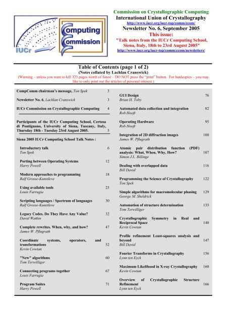
Commission on Crystallographic Computing<br />
<strong>International</strong> <strong>Union</strong> <strong>of</strong> Crystallography<br />
http://www.iucr.org/iucr-top/comm/ccom/<br />
Newsletter No. 6, September 2005<br />
This issue:<br />
"Talk notes from the IUCr Computing School,<br />
Siena, Italy, 18th to 23rd August 2005"<br />
http://www.iucr.org/iucr-top/comm/ccom/newsletters/<br />
<strong>Table</strong> <strong>of</strong> <strong>Contents</strong> (<strong>page</strong> 1 <strong>of</strong> 2)<br />
(Notes collated by Lachlan Cranswick)<br />
(Warning – unless you want to kill 323 <strong>page</strong>s worth <strong>of</strong> forest – DO NOT press the “print” button. For hardcopies – you may<br />
like to only print out the articles <strong>of</strong> personal interest.)<br />
CompComm chairman’s message, Ton Spek 3<br />
Newsletter No. 6, Lachlan Cranswick 3<br />
IUCr Commission on Crystallographic Computing 4<br />
Participants <strong>of</strong> the IUCr Computing School, Certosa<br />
di Pontignano, University <strong>of</strong> Siena, Tuscany, Italy,<br />
Thursday 18th - Tuesday 23rd August 2005. 5<br />
Siena 2005 IUCr Computing School Talk Notes :<br />
Introductory talk 6<br />
Ton Spek<br />
Porting between Operating Systems 12<br />
Harry Powell<br />
Modern approaches to programming 18<br />
Ralf Grosse-Kunstleve<br />
Using available tools 23<br />
Louis Farrugia<br />
Scripting languages / Spectrum <strong>of</strong> languages 30<br />
Ralf Grosse-Kunstleve<br />
Legacy Codes. Do They Have Any Value? 32<br />
David Watkin<br />
Complete rewrites. When, why, and how? 47<br />
James W. Pflugrath<br />
Coordinate systems, operators, and<br />
transformations 52<br />
Kevin Cowtan<br />
"New" algorithms 60<br />
Tom Terwilliger<br />
Connecting programs together 67<br />
Louis Farrugia<br />
Program Suites 71<br />
Harry Powell<br />
GUI Design 76<br />
Brian H. Toby<br />
Automated data collection and integration 82<br />
Rob Ho<strong>of</strong>t<br />
Operating Hardware 95<br />
Rob Ho<strong>of</strong>t<br />
Integration <strong>of</strong> 2D diffraction images 100<br />
James W. Pflugrath<br />
Atomic pair distribution function (PDF)<br />
analysis: What, When, Why, How? 107<br />
Simon J.L. Billinge<br />
Dealing with overlapped data 116<br />
Bill David<br />
Programming the Science <strong>of</strong> Crystallography 122<br />
Ton Spek<br />
Simple algorithms for macromolecular phasing 129<br />
George M. Sheldrick<br />
Automation <strong>of</strong> structure determination 133<br />
Tom Terwilliger<br />
Crystallographic Symmetry in Real and<br />
Reciprocal Space 140<br />
Kevin Cowtan<br />
Pr<strong>of</strong>ile refinement Least-squares analysis and<br />
beyond 147<br />
Bill David<br />
Fourier Transforms in Crystallography 156<br />
Lynn ten Eyck<br />
Maximum Likelihood in X-ray Crystallography 160<br />
Kevin Cowtan<br />
Overview <strong>of</strong> Crystallographic Structure<br />
Refinement 166<br />
Lynn ten Eyck
Refinement II - Modern Developments 168<br />
Dale E. Tronrud<br />
CCP14 workshop Notes: On Minimization<br />
Targets and Algorithms 171<br />
Dale E. Tronrud<br />
Computational aspects <strong>of</strong> the Rietveld Method 176<br />
Juan Rodríguez-Carvajal<br />
Statistical Treatment <strong>of</strong> Uncertainties 183<br />
Dale E. Tronrud<br />
Programming pdCIF and Rietveld 187<br />
Brian H. Toby<br />
Structure Comparison, Analysis and Validation 194<br />
Ton Spek<br />
Testing s<strong>of</strong>tware 202<br />
Harry Powell<br />
The future <strong>of</strong> direct methods 206<br />
George M. Sheldrick<br />
CrysFML: A crystallographic library in modern<br />
Fortran 271<br />
Juan Rodríguez-Carvajal<br />
Connecting to hardware 280<br />
Rob Ho<strong>of</strong>t<br />
Tcl/Tk demo 286<br />
Brian Toby<br />
CCTBX Unit Cell Refinement Tutorial 292<br />
Ralf W. Grosse-Kunstleve<br />
CCTBX Direct Methods Tutorial 303<br />
Ralf W. Grosse-Kunstleve<br />
CCTBX Central Types 317<br />
Ralf W. Grosse-Kunstleve<br />
Tutorial on scoring methods for evaluation <strong>of</strong><br />
electron density maps 318<br />
Tom Terwilliger<br />
Siena 2005 IUCr Computing School Tutorials :<br />
Calls for contributions to Newsletter No. 7 323<br />
Using the Clipper libraries 210<br />
Kevin Cowtan<br />
Exercises in map manipulation 220<br />
Kevin Cowtan<br />
Reciprocal Space Tutorial (RST) 224<br />
George M. Sheldrick<br />
Fortran 77 solution to GMS RST 229<br />
George M. Sheldrick<br />
C++ solution to GMS RST 232<br />
Tim Gruene<br />
C++ solution to GMS RST 239<br />
Michel Fodje<br />
Fortran 95 solution to GMS RST 247<br />
Juan Rodríguez-Carvajal<br />
Java solution to GMS RST 252<br />
Bradley Smith<br />
Fortran solution to GMS RST 258<br />
Stephan Ruehl<br />
Initial Python solution to GMS RST 269<br />
Ralf W. Grosse-Kunstleve<br />
Slightly Enhanced Python solution to GMS RST 270<br />
Ralf W. Grosse-Kunstleve<br />
Page 2
CompComm Chairman’s Message<br />
This newsletter makes the presentations available to a wider audience <strong>of</strong> the lectures given at the IUCr<br />
Crystallographic Computing School 2005 in Siena, prior to the Florence 2005 IUCr congress. This<br />
breaks with a tradition <strong>of</strong> the past where, based on the material presented, a very expensive book was<br />
produced with rather limited distribution. We hope that the current approach that we have choosen for<br />
the distribution <strong>of</strong> the lecture material fits more in our 'Google-age', where a lot <strong>of</strong> information is now<br />
looked for on the WEB.<br />
One <strong>of</strong> the implicit themes during this meeting was the s<strong>of</strong>tware language to be used for future s<strong>of</strong>tware<br />
development. Traditionally, Fortran in its various incarnations was the default language. A large number<br />
<strong>of</strong> programs that are in use today are written in that language (e.g. the SHELX suite). Fortran could still<br />
be the language <strong>of</strong> choice today for scientific computing in view <strong>of</strong> its simplicity and efficiency.<br />
However, computing science has now moved to C-type and scripting languages, <strong>of</strong> which C++ and<br />
Python are currently the most popular respectively. A large number <strong>of</strong> libraries for graphical user<br />
interfaces are currently available for those languages. C++ will be the de-facto language <strong>of</strong> the future,<br />
notwithstanding its sharp learning curve. Interestingly, George Sheldrick (one <strong>of</strong> the lecturers and a<br />
longstanding Fortran addict like me) has now taught himself C++ as an outcome <strong>of</strong> this very successfull<br />
school.<br />
I would like to thank the speakers again for all the work they did to prepare their presentations, the<br />
sponsors for their financial support, my co-organisers, the University <strong>of</strong> Siena for making available an<br />
excellent meeting site and Pr<strong>of</strong>. Marcello Mellini for making it all work locally.<br />
Ton Spek, Chairman <strong>of</strong> the IUCR computing school and IUCr Computing Commission,<br />
(a.l.spek@chem.uu.nl )<br />
Newsletter No. 6<br />
This newsletter collates the notes from the Siena 2005 IUCr Crystallographic Computing School. The<br />
individual files are located on the school web<strong>page</strong> at:<br />
http://www.iucr.org/iucr-top/comm/ccom/siena2005/notes.html<br />
The next edition <strong>of</strong> the newsletter is expected to get back to the usual format with an intended theme<br />
involving “Minimisation” algorithms for indexing, structure solution and refinement. It should hopefully<br />
appear around April 2006.<br />
Lachlan Cranswick,<br />
(lachlan.cranswick@nrc.gc.ca)<br />
Page 3
THE IUCR COMMISSION ON CRYSTALLOGRAPHIC COMPUTING - TRIENNIUM 2005-2008<br />
Chairman: Pr<strong>of</strong>essor Dr. Anthony L. Spek<br />
Director <strong>of</strong> National Single Crystal Service Facility,<br />
Utrecht University,<br />
H.R. Kruytgebouw, N-801,<br />
Padualaan 8, 3584 CH Utrecht,<br />
the Netherlands.<br />
Tel: +31-30-2532538<br />
Fax: +31-30-2533940<br />
E-mail: a.l.spek@chem.uu.nl<br />
WWW: http://www.cryst.chem.uu.nl/spea.html<br />
Lachlan M. D. Cranswick<br />
Canadian Neutron Beam Centre (CNBC),<br />
National Research Council (NRC),<br />
Building 459, Station 18, Chalk River Laboratories,<br />
Chalk River, Ontario, Canada, K0J 1J0<br />
Tel: (613) 584-8811 ext: 3719<br />
Fax: (613) 584-4040<br />
E-mail: lachlan.cranswick@nrc.gc.ca<br />
WWW: http://neutron.nrc.gc.ca/peep.html#cranswick<br />
Dr Ralf W. Grosse-Kunstleve<br />
Lawrence Berkeley National Laboratory<br />
One Cyclotron Road, BLDG 64R0121,<br />
Berkeley, California, 94720-8118, USA.<br />
Tel: (510) 486-5929<br />
Fax: (510) 486-5909<br />
E-mail: RWGrosse-Kunstleve@lbl.gov<br />
WWW: http://cci.lbl.gov/<br />
Pr<strong>of</strong>essor Alessandro Gualtieri<br />
Università di Modena e Reggio Emilia,<br />
Dipartimento di Scienze della Terra,<br />
Via S.Eufemia, 19,<br />
41100 Modena, Italy<br />
Tel: +39-059-2055810<br />
Fax: +39-059-2055887<br />
E-mail: alex@unimore.it<br />
WWW: http://www.terra.unimo.it/mineralogia/gualtieri.html<br />
Pr<strong>of</strong>essor Luhua Lai<br />
Institute <strong>of</strong> Physical Chemistry,<br />
Peking University,<br />
Beijing 100871,<br />
China.<br />
Fax: +86-10-62751725.<br />
E-mail: lhlai@pku.edu.cn<br />
WWW: http://mdl.ipc.pku.edu.cn/<br />
Dr Airlie McCoy<br />
Structural Medicine,<br />
Cambridge Institute for Medical Research (CIMR),<br />
Wellcome Trust/MRC Building,<br />
Addenbrooke's Hospital, Hills Road, Cambridge CB2 2XY, UK<br />
Tel: +44 (0) 1223 217124<br />
Fax: +44 (0) 1223 217017<br />
E-mail: ajm201@cam.ac.uk<br />
WWW: http://www-structmed.cimr.cam.ac.uk/<br />
Pr<strong>of</strong>essor Atsushi Nakagawa<br />
Research Center for Structural and Functional Proteomics,<br />
Institute for Protein Research,<br />
Osaka University,<br />
3-2 Yamadaoka, Suita,<br />
Osaka, 565-0871, Japan<br />
Tel: +81-(0)6-6879-4313<br />
Fax: +81-(0)6-6879-4313<br />
E-mail: atsushi@protein.osaka-u.ac.jp<br />
WWW: http://www.protein.osaka-u.ac.jp/<br />
Dr. Simon Parsons<br />
School <strong>of</strong> Chemistry, University <strong>of</strong> Edinburgh<br />
Joseph Black Building, West Mains Road,<br />
Edinburgh, Scotland EH9 3JJ, UK<br />
Tel: +44 131 650 5804<br />
Fax: +44 131 650 4743<br />
E-mail: s.parsons@ed.ac.uk<br />
WWW: http://www.chem.ed.ac.uk/staff/parsons.html<br />
Dr Harry Powell<br />
MRC Laboratory <strong>of</strong> Molecular Biology,<br />
Hills Road, Cambridge, CB2 2QH, UK.<br />
Tel: +44 (0) 1223 248011<br />
Fax: +44 (0) 1223 213556<br />
E-mail: harry@mrc-lmb.cam.ac.uk<br />
WWW: http://www.mrc-lmb.cam.ac.uk/harry/<br />
Consultants<br />
Pr<strong>of</strong>essor I. David Brown<br />
Brockhouse Institute for Materials Research,<br />
McMaster University, Hamilton, Ontario, Canada<br />
Tel: 1-(905)-525-9140 ext 24710<br />
Fax: 1-(905)-521-2773<br />
E-mail: idbrown@mcmaster.ca<br />
WWW: http://www.physics.mcmaster.ca/people/faculty/Brown_ID_h.html<br />
Pr<strong>of</strong>essor Eleanor Dodson<br />
York Structural Biology Laboratory,<br />
Department Of Chemistry,<br />
University <strong>of</strong> York, Heslington,<br />
York, YO10 5YW, UK<br />
Tel: +44 (1904) 328253<br />
Fax: +44 1904 328266<br />
E-mail: e.dodson@ysbl.york.ac.uk<br />
WWW: http://www.ysbl.york.ac.uk/people/6.htm<br />
Dr David Watkin<br />
Chemical Crystallography, Department <strong>of</strong> Chemistry,<br />
University <strong>of</strong> Oxford, Chemistry Research Laboratory,<br />
Mansfield Road,<br />
Oxford, OX1 3TA, UK<br />
Tel: +44 (0) 1865 285019<br />
Fax: +44 (0) 1865 285021<br />
E-mail: david.watkin@chemistry.oxford.ac.uk<br />
WWW: http://www.chem.ox.ac.uk/researchguide/djwatkin.html<br />
Page 4
Participants <strong>of</strong> the IUCr Computing School, Certosa di Pontignano,<br />
University <strong>of</strong> Siena, Tuscany, Italy, Thursday 18th - Tuesday 23rd August<br />
2005.<br />
Organisers: Ton Spek, Marcello Mellini, Alessandro Gualtieri, Harry Powell, Lachlan Cranswick<br />
Consultants: Simon Parsons, David Watkin<br />
IUCr Representative: Davide Viterbo<br />
Lecturers: Simon Billinge, Kevin Cowtan, Bill David, Louis Farrugia, Ralf Grosse-Kunstleve, Rob<br />
Ho<strong>of</strong>t, James Pfugrath, Harry Powell, Juan Rodríguez-Carvajal, George Sheldrick, Ton Spek, Lynn ten<br />
Eyck, Tom Terwilliger, Brian Toby, Dale Tronrud, David Watkin<br />
Registrants: Priyamvada Acharya, Sandor Brockhauser, Jeppe Christensen, Jeremy Cockcr<strong>of</strong>t, Fabio<br />
Dall'Antonia, Paul Emsley, ZhenJie Feng, Laura Roces Fernández, Laura Torre Fernández, Marc<br />
Fleurant, Michel Fodje, Frantisek Frantisek, Nicholas Furnham, Roni Gordon, Tim Gruene, Carmen<br />
Guguta, Ilia Guzei, Svetlana Ivashevskaya, Soorya N Kabekkodu, Huub Kooijman, Gert J. Kruger,<br />
Maciej Kubicki, Martin Lutz, Yvonne P. Mascarenhas, Ernesto Mesto, Alexander Nazarenko, Steven<br />
Ness, Aritra Pal, Pryank Patel, Simon Parsons, Mike Probert, Cristy Leonor Azanza Ricardo, Stephan<br />
Ruehl, Irakli Sikharulidze, Pavol Skubak, Alexander B. Smith, Bradley Smith, Margareta Sorenson,<br />
Richard Stephenson, Gudrun Stranzl, Pavel Teslenko, Michael Turner, Peter Turner, Marco Voltolini,<br />
Marcin Wojdyr, Pete Wood, Jon Wright, Xinyi Xian,<br />
Accompanying Persons: Linda ten Eyck, Aviva Pelt, Katherine Sheldrick<br />
Sponsors:<br />
Università di Siena<br />
MAX-INF2<br />
Merck & Co., Inc. - USA<br />
Bruker AXS<br />
Cambridge Crystallographic Data Centre (CCDC)<br />
CCP4 - Collaborative Computing Project Number 4 in Protein Crystallography<br />
Oxford Diffraction<br />
Rigaku/MSC<br />
<strong>International</strong> <strong>Union</strong> <strong>of</strong> Crystallography (IUCr)<br />
Page 5
Some History<br />
INTRODUCTORY TALK<br />
Ton Spek<br />
National Single Crystal Service<br />
Facility<br />
Utrecht University<br />
• On crystallographic computing from the perspective <strong>of</strong> a<br />
small-molecule crystallographer who started to work in<br />
crystallography in the mid 60’s at Utrecht University, The<br />
Netherlands.<br />
• Many <strong>of</strong> the older s<strong>of</strong>tware developers, like me, have a<br />
background in Direct Methods. Mine started as follows:<br />
• As a student, I was given a colorless crystal <strong>of</strong> unknown<br />
composition with the assignment to determine its structure<br />
using X-ray techniques only. It took me more than ½ a<br />
year to determine that it was methoxyglutaconic acid.<br />
• Today, 40 years later, a problem like this is solved in a<br />
matter <strong>of</strong> seconds on my notebook, but not in those days.<br />
Not so 40 Years ago<br />
• The crystallography group in Utrecht already had a tradition in Direct<br />
Methods (Paul Beurskens, one <strong>of</strong> the first authors implementing the<br />
Symbolic Addition Method). However, none <strong>of</strong> the locally available<br />
programs gave an interpretable hand-contoured map.<br />
• So I ended up with developing my own Symbolic Addition program,<br />
AUDICE, for centro-symmetric structures.<br />
• AUDICE was locally rather successful since it also solved all other<br />
notoriously ‘unsolvable structures’ hanging around in the lab.<br />
• Major calculations and program testing were done once a week during<br />
the ‘nightshift’, not ‘overnight’, on the Utrecht University mainframe.<br />
(A major social event in those days in view <strong>of</strong> the presence <strong>of</strong> most<br />
group members between 6PM and 8 AM the next morning)<br />
16kW<br />
~1966, Electrologica X8 ALGOL60 ‘Mainframe’ (
Direct Methods Meetings<br />
• Many past meetings and schools were organized with<br />
Direct Methods (s<strong>of</strong>tware and theory) as a major subject.<br />
• Important one’s were the CECAM workshops on Direct<br />
Methods (5 weeks!, bringing together people working in<br />
the field to work on current issues) in the early 70’s in<br />
Orsay around a big IBM-360 with lectures by Hauptman.<br />
• Launch <strong>of</strong> MULTAN, many personal contacts – Viterbo<br />
• NATO schools on Direct Methods in Parma and York in<br />
the 70’s.<br />
• Direct Methods schools in Erice in 1974 & 1978.<br />
• Photo <strong>of</strong> the participants <strong>of</strong> the 1978 Erice School next :<br />
Direct Methods Now<br />
IUCr Computing Schools<br />
• Direct Methods appear to be currently no longer a major<br />
topic at meetings.<br />
• Some years ago there was a morning lecture by Herbert<br />
Hauptman with the message that the tangent formula was<br />
what really mattered. That afternoon there was as lecture<br />
by Carmello Giacovazzo with the message that there was<br />
no need for the tangent formula…<br />
• George Sheldrick will give us his perspective on ‘The<br />
Future <strong>of</strong> Direct Methods’ at the end <strong>of</strong> this meeting.<br />
• ….. Mostly held jointly with IUCr Assemblies – Examples<br />
• 1963 – Rollett, Algorithms (black book)<br />
• 1969 - Least-Squares & Absorption Correction (SHELX76 - code)<br />
• 1978 - Program systems (SHELX, XTAL, NRCVAX etc.)<br />
• 1996 - Macro-crystallography<br />
• 1999 - Macro-crystallography<br />
• 2002 – (None)<br />
• 2005 - Siena (again: Small, Macro, Powder)<br />
• Photo 1978 school in Enschede (Netherlands)<br />
Motivations for this Crystallographic<br />
Computing School<br />
• A general feeling within at least the small-molecule community:<br />
‘The current generation <strong>of</strong> s<strong>of</strong>tware developers is phasing out, where is<br />
the new generation to keep things running in the future’<br />
• There exists a growing community <strong>of</strong> push-button users<br />
(What is not behind a button can not be done…)<br />
• Major funding and s<strong>of</strong>tware development is currently in macro<br />
crystallography<br />
(possible useful spin-<strong>of</strong>f to the small-molecule world)<br />
• It is sensed that things well known in the small-molecule world are<br />
reinvented in the macro world and presented as new.<br />
• Black Box and Proprietary S<strong>of</strong>tware as opposed to Open Source.<br />
(lack <strong>of</strong> info about the algorithms used and options to modify)<br />
Page 7
Hardware Platforms<br />
• MS-Windows:<br />
Small-Molecule Crystallography<br />
Powder crystallography<br />
• UNIX/LINUX/(OSX):<br />
Macro Crystallography<br />
(Small-Molecule Crystallography)<br />
S<strong>of</strong>tware Languages<br />
• Crystallographic s<strong>of</strong>tware has been written in machine language,<br />
assembly language, algol60, (turbo)basic, (turbo)pascal, Fortran, C,<br />
C++ and various scripting languages such as python<br />
• ‘Stone-age’ Fortran based s<strong>of</strong>tware is still ubiquitous in the smallmolecule<br />
world (ORTEP, SHELX, CRYSTALS, PLATON etc.)<br />
• New (commercial) s<strong>of</strong>tware development mainly in C++ and scripting<br />
languages.<br />
• A project just started in the UK to Rethink & Rewrite old Fortran<br />
based s<strong>of</strong>tware to C++ (Durham, Oxford project).<br />
• Old s<strong>of</strong>tware saved in ‘The Crystallographic Source Code Museum’ by<br />
Armal LeBail, supposedly interesting to look for useful algorithms.<br />
SHELX76-STYLE FORTRAN<br />
Alternative Algorithms for the<br />
Implementation <strong>of</strong> the same Task<br />
• Tasks can usually be programmed in a variety <strong>of</strong> ways<br />
with widely ranging claims on memory and CPU<br />
resources.<br />
• It is important to know the actual application to make the<br />
relevant decisions.<br />
• Following is a simple, though somewhat extreme, example<br />
from the 1960’s where a theoretical idea in Direct Methods<br />
was given to a pr<strong>of</strong>essional programmer to implement.<br />
• The final program was nicely written and documented.<br />
• However, the calculation didn’t terminate within hours<br />
even for a trivial application ….(my mystery structure)<br />
Page 8
Problem from Symbolic Addition Method<br />
P+ for triple H,K,H+K depends on<br />
|E(H)E(K)E(H+K)|<br />
Two Implementations<br />
L<br />
H<br />
K<br />
H+K<br />
‘Correlation Method’ Improved P+<br />
on the basis <strong>of</strong> P+ <strong>of</strong> three adjacent triples<br />
|E(H)E(L)E(H+L)|<br />
|E(K)E(L-K)E(L)|<br />
|E(H+K)E(L-K)E(H+L)|<br />
I.e. Strengthening <strong>of</strong> P+(|E(H)E(K)E(H+K)|<br />
when in addition E(H+L),E(L-K),E(L) strong<br />
(Note: Theoretically formalized in terms <strong>of</strong><br />
neighbourhoods, Hauptman)<br />
• Implementation I: (Pr<strong>of</strong>essional Programmer)<br />
1 - Search and store all triple products found with E ><br />
E(min)<br />
2 - Find from this list quartets <strong>of</strong> triples forming a<br />
tetrahedron<br />
Problem with 1: The number <strong>of</strong> triplets explodes with<br />
increasing size <strong>of</strong> the structure at hand and so memory<br />
requirements (limited to 16kW in those days)<br />
Problem with 2: Multiple nested loops with large range<br />
L<br />
H<br />
K<br />
H+K<br />
Implementation II (by Young Student)<br />
Generate ‘correlations’ on the fly during<br />
triple relation search by looping with L<br />
with E(L) > E(min) and testing for large<br />
E(L-K) and E(H+L).<br />
Result: Completion <strong>of</strong> the search in<br />
minutes rather than hours.<br />
Numerical Recipes<br />
• An excellent and rich source <strong>of</strong> numerical<br />
routines for sorting, optimisation, FFT etc.<br />
with associated background is the book<br />
Numerical Recipes by W.H. Press et al.,<br />
that has separate Fortran and C versions<br />
Numerical Recipe Example<br />
• A very nice routine from NR is code with<br />
the name ‘FOURN.FOR’.<br />
• Forward and Backward FFT in N<br />
dimensions.<br />
• In our crystallographic application: N = 3<br />
• Code = 69 Fortran lines ! Next ….<br />
Page 9
Application <strong>of</strong> FOURN.FOR<br />
• Ab Initio structure solution by charge flipping<br />
• See G.Oszlanyi & A. Suto, (2004) Acta Cryst A60,134.<br />
• Procedure: cycle between reciprocal space to direct space<br />
and back after modification <strong>of</strong> the density map until<br />
convergence using forward and backward FFT.<br />
So, No More D.M. ?<br />
• Preliminary results on real structures,<br />
including incommensurate structures look<br />
interesting.<br />
• There will be a lecture on this in Florence<br />
(MS20).<br />
• Faster FFT: (Free C-library) FFTW<br />
However, with greater implementation and<br />
portability complexities.<br />
Other Computing Areas<br />
• Powder (indexing, solution, refinement)<br />
• RDF (Billinge)<br />
• Macro Xtal (Phasing, Building,<br />
Refinement)<br />
• Charge Density Studies (XD)<br />
• Least Squares and other optimisation<br />
techniques.<br />
Other Computing Areas<br />
• Incommensurate Structures (solution,<br />
refinement) (Keynote lecture by Petricek in<br />
Florence).<br />
• Graphics (GUI’s and presentation)<br />
• Data collection and data reduction.<br />
• Databases, Structure analysis and<br />
Validation<br />
The Program <strong>of</strong> the School<br />
• There has been some discussion in the program<br />
commission on whether there should be two<br />
largely parallel sessions in view <strong>of</strong> a perceived<br />
growing diversion <strong>of</strong> interest.<br />
• Eventually this path was not pursued, resulting in<br />
the current program that involves a mix <strong>of</strong> smallmolecule,<br />
macro-molecule and powder interests.<br />
• This format should provide a fruitful platform to<br />
pick up and discuss ideas from each others field.<br />
The Program <strong>of</strong> the School<br />
• Lecturers were asked to focus on s<strong>of</strong>tware development<br />
and internals rather than presenting the latest science or<br />
user instruction to their s<strong>of</strong>tware.<br />
• Not a school to learn basic programming.<br />
• An introduction to current s<strong>of</strong>tware development<br />
techniques (scripting languages, toolboxes etc.)<br />
• Hands-on projects and workshops on personal notebooks.<br />
• Bringing together representatives <strong>of</strong> the older and a next<br />
generation interested in s<strong>of</strong>tware development.<br />
Page 10
Thanks to our Sponsors !<br />
• Bruker-Nonius AXS<br />
• Cambridge Crystallographic Data Center<br />
• CCP4<br />
• IUCr<br />
• Max-Inf2<br />
• Merck & Co., Inc, USA<br />
• Oxford Diffraction<br />
• Rigaku/MSC<br />
• Universita degli Studi di Siena<br />
Page 11
Porting between Operating Systems<br />
or<br />
how to increase your customer base<br />
Why bother to port (doesn’t everyone use MS-Windows)?<br />
- support a wider community (some people use other<br />
platforms) - more people will use your s<strong>of</strong>tware<br />
- future pro<strong>of</strong>ing (remember DEC VAX or PDP-11? or IBM<br />
370/168?)<br />
- leads to more standard code (which should be more<br />
maintainable)<br />
Harry Powell MRC-LMB<br />
Which platforms/operating systems to port to? This depends<br />
on:<br />
- who you want to use your s<strong>of</strong>tware (most important)<br />
- what hardware you have available for building/testing<br />
Serious developers will usually have access to:<br />
• PC / Linux (no excuse for not having it!)<br />
• PC / MS-Windows (probably)<br />
• Mac / OS X (becoming more popular)<br />
• SGI / Irix (historically important)<br />
• Alpha / Tru64 (historically important)<br />
• Sun /Solaris or SunOS (niche product in crystallography)<br />
• HP-UX (niche product in crystallography)<br />
Three basic types <strong>of</strong> porting;<br />
1. existing s<strong>of</strong>tware<br />
2. new graphical interfaces<br />
3. functionality<br />
Porting Existing S<strong>of</strong>tware<br />
Assumption that a complete re-write is not<br />
necessary/appropriate/desired<br />
Porting existing s<strong>of</strong>tware<br />
Reasons include:<br />
this program is<br />
• mature;<br />
• does its job;<br />
• will not be developed much further;<br />
• enormous (any re-write will take many man-years &<br />
introduce many bugs)<br />
• obsolescent (i.e. it will be rewritten when time permits)<br />
Page 12
Porting Existing S<strong>of</strong>tware<br />
Used to be expensive/difficult - only readily available compilers<br />
were commercial and tied to a platform, had useful platform<br />
dependent features (e.g. VAX FORTRAN)<br />
Now platforms exist which have a “free” development<br />
environment (e.g. Linux, Mac OS X, Cygwin/MinGW)<br />
“Free” compilers which adhere to the standards now exist<br />
(gcc/g77 for most platforms, Salford FTN77 for MS-<br />
Windows, icc/ifc for Intel Linux)<br />
Porting Existing S<strong>of</strong>tware<br />
Why use a commercial compiler?<br />
• “You get what you pay for”<br />
• user support<br />
• <strong>of</strong>ten better optimization (for specific platforms)<br />
• good development environments (e.g. Visual Studio)<br />
• your institution/company may already have paid for and<br />
own a licence<br />
Porting Existing S<strong>of</strong>tware<br />
Why use a “free” compiler?<br />
• low initial cost<br />
• modern ones <strong>of</strong>ten produce executables about as fast as<br />
commercial ones<br />
• same compiler across multiple platforms<br />
• readily available cross compilers (build on Linux, run on<br />
Windows - or vice versa)<br />
• good development environments (e.g. XEmacs)<br />
but - you get what you pay for, so it can be buggy - e.g. gcc 2.96<br />
distributed with Red Hat Linux should never have been<br />
released<br />
Porting from MS-Windows to other systems<br />
• need a system to build on<br />
• need a system to test on<br />
Possible to cross-develop on MS-Windows but the target<br />
windowing system will be different.<br />
Two easy routes -<br />
1. install Linux and dual boot (best environment)<br />
2. install Cygwin (easiest since you can run MS-Windows<br />
simultaneously)<br />
Each <strong>of</strong> these provides a fully-featured windowed environment<br />
via X11 windows, but Cygwin will produce MS-Windows<br />
executables unless you cross-compile!<br />
Page 13
Porting from any UNIX to other systems<br />
• “easy” if the other system is UNIX-based<br />
• can be an opportunity to modularize functionality<br />
• for MS-Windows need a system (probably not a problem for<br />
most people):<br />
Choices:<br />
• MinGW (Minimalist GNU for Windows), provides<br />
compilation tools under Windows<br />
• Cygwin; easy to migrate a UNIX build (essentially<br />
identical to Linux on PC)<br />
• Cross-compilers; build under system A, run on system<br />
B.<br />
Problems with porting (1):<br />
It will probably identify bugs in your code (some “strict”<br />
compilers are stricter than others):<br />
WRITE(*,*),’hello world’<br />
compiles as expected with f77 on Tru64 UNIX, g77 on Linux &<br />
MacOS, but not with xlf on MacOS.<br />
WRITE(*,*)’hello world’;<br />
compiles as expected with f77 on Tru64 UNIX, g77 on Linux &<br />
MacOS, xlf on MacOS, but not on Irix with f77 (because it's<br />
actually f90).<br />
Problems with porting (2):<br />
May identify bugs in compilers - e.g. file “break.f” contains the<br />
following:<br />
CHARACTER*2 TEST(2)<br />
CHARACTER*1 JUNK<br />
JUNK = 'O'<br />
WRITE(TEST,FMT=1000)JUNK<br />
1000 FORMAT(A)<br />
END<br />
[g4-15:~/programs] harry% gfortran -c break.f<br />
break.f: In function 'MAIN__':<br />
break.f:3: internal compiler error: Bus error<br />
Please submit a full bug report,<br />
with preprocessed source if appropriate.<br />
See for instructions.<br />
Problems with porting (3):<br />
If you can't distribute static binaries, your customer's computers<br />
are probably missing vital libraries, shared objects, and<br />
other bits and pieces necessary to run your code which you<br />
(a) didn't think were necessary<br />
(b) assumed were ubiquitous<br />
(c) hadn't even thought about<br />
They might be there, but are from an older/newer version <strong>of</strong> the<br />
operating system and are therefore incompatible.<br />
This can lead to a new career in compiler development!<br />
Problems with porting (5):<br />
Problems with porting (4):<br />
You may feel that months <strong>of</strong> work may be wasted when a<br />
manufacturer makes a major change to its hardware or<br />
operating system, e.g.<br />
Apple - OS X made all previous Apple s<strong>of</strong>tware obsolete<br />
Apple - change <strong>of</strong> processor from PowerPC to Intel makes<br />
xlc/xlf compiler specific work obsolete.<br />
Porting to (and from) MS-Windows is probably the most<br />
difficult step because <strong>of</strong> its unique environment; all other<br />
popular platforms share a similar operating system and have<br />
available a similar windowing system.<br />
For example, identical code for Mosflm* (150,000 lines <strong>of</strong><br />
Fortran, 100,000 lines <strong>of</strong> C, + 80,000 lines <strong>of</strong> graphics<br />
library) builds using the same commands on all UNIX<br />
boxes, but without tools like Cygwin requires a major<br />
restructuring for MS-Windows.<br />
* a popular data integration program<br />
Page 14
Command-line interfaces - old-fashioned but generally<br />
straightforward; however, MS-Windows users won't like it!<br />
Graphical interfaces - need to distinguish between<br />
new graphical interfaces<br />
• windowing environment - most platform dependent<br />
• MS-Windows - tied to Windows PCs<br />
• Aqua - tied to Macintosh<br />
• X11 - can be used on anything it’s been ported to<br />
• interface utilities -<br />
• Tk (Tcl/Tk, Tkinter, ...)<br />
• wxWidgets (was wxWindows), Qt, Clearwin...<br />
• browser applets<br />
For portability we need the utility to have been ported to the<br />
environment (or the environment to have been ported to the<br />
platform)<br />
The current Mosflm approach to a GUI -<br />
1. uses a custom-built (obsolete) X11 widget set - xdl_view<br />
2. compile to create a monolithic program<br />
Pros:<br />
• distribution <strong>of</strong> the executable is easy (no need for extra libraries<br />
for the GUI)<br />
• familiar widget set (for the programmer, anyway)<br />
Cons:<br />
• development <strong>of</strong> both Mosflm and the GUI are intimately linked<br />
• “hard” to port to OS’s without an X-server<br />
• xdl_view can behave subtly differently on different OS’s -<br />
relied on some benign features <strong>of</strong> compilers<br />
Portable interface utilities 1 - Tcl/Tk<br />
The new Mosflm approach to a GUI;<br />
1. core crystallographic functions (controlled by command line<br />
instructions)<br />
2. A Tcl/Tk GUI which reads XML and writes native Mosflm<br />
commands<br />
3. the two parts communicate via TCP/IP sockets<br />
Pros:<br />
• Mosflm can be run on any platform independently <strong>of</strong> the<br />
GUI<br />
• development <strong>of</strong> both Mosflm and the GUI can proceed<br />
semi-independently<br />
mature but losing popularity; development in some important<br />
modules is almost non-existent (e.g. incrTcl).<br />
Installation <strong>of</strong> Tcl/Tk based programs may require additional<br />
packages to be installed (e.g. TkImg), but some are not<br />
available for all platforms (e.g. BLT is not available for<br />
Aqua).<br />
Tkinter is Python's de facto standard GUI package. It is a thin<br />
object-oriented layer on top <strong>of</strong> Tcl/Tk.<br />
can interface with compiled code via 4 basic routes -<br />
1. embed compiled code into Tcl/Tk script<br />
2. run external programs directly from the script<br />
3. read from & write to a file<br />
4. read from & write to a TCP/IP socket<br />
Page 15
Portable interface utilities 2 - wxWidgets<br />
Set <strong>of</strong> C++ class libraries<br />
Main differences from Tcl/Tk:<br />
• encourages an object oriented approach<br />
• the GUI can be compiled so that the programming details<br />
can be hidden from the user; also this can give a<br />
performance advantage, especially for interactive graphics.<br />
Gives a native look and feel on different platforms, usable with<br />
any common C++<br />
wxPython is “a blending <strong>of</strong> wxWidgets with Python” - used in<br />
PHENIX<br />
A popular small molecule<br />
program running on Windows and<br />
Linux<br />
Could be viewed as a new project - coding from scratch -<br />
probably best to use new languages (C++, Python, Java)<br />
rather than established languages.<br />
Porting functionality<br />
What you use depends on the application to some extent, e.g.<br />
web applications - Java<br />
heavyweight applications - C++<br />
prototyping - Python<br />
If you have a free choice at this point, development can be faster<br />
and portable features can be designed in.<br />
Why not just use FORTRAN?<br />
- fast executables with little effort<br />
- many applications/libraries available<br />
- well-established amongst senior scientists<br />
- F90, 95, 200x have modern programming constructs<br />
Why shouldn’t you use FORTRAN?<br />
- can quickly lead to spaghetti code<br />
- possible lack <strong>of</strong> long-term maintainability<br />
- little support from “real” programmers (it isn’t taught in CS<br />
departments!)<br />
- modern languages make development faster<br />
- good OOP imposes modularity<br />
Page 16
Don’t re-invent the wheel unnecessarily - there is a whole host<br />
<strong>of</strong> functionality which has already been coded (s<strong>of</strong>tware<br />
libraries for underlying crystallographic operations) - but<br />
there may be licensing issues.<br />
Code can be cribbed from books (e.g. “Numerical Recipes”) but<br />
be aware <strong>of</strong> copyright issues.<br />
Other developers may be willing to "give" you their code for<br />
inclusion (e.g. both autoindexing routines in Mosflm)<br />
Finally -<br />
Design in portability -<br />
• don’t use platform specific features if possible<br />
• use standard programming contructs<br />
• gcc/g77/g++ is available for virtually every platform -<br />
essentially the same build can be used (some compiler flags<br />
and libraries may differ)<br />
Page 17
Siena Computational Crystallography School 2005<br />
Modern approaches to programming<br />
Ralf W. Grosse-Kunstleve<br />
Computational Crystallography Initiative<br />
Lawrence Berkeley National Laboratory<br />
Disclosure<br />
• Experience<br />
– Basic<br />
– 6502 machine language<br />
– Pascal<br />
– Fortran 77<br />
– csh, sh<br />
– C<br />
– Perl<br />
– Python<br />
– C++<br />
• Last five years<br />
– Python & C++ -> cctbx, phenix<br />
• Development focus<br />
– phenix.refine, phenix.hyss<br />
• No experience<br />
– TCL/TK<br />
– Java<br />
Computational Crystallography Toolbox<br />
• Open-source component <strong>of</strong> phenix<br />
– Automation <strong>of</strong> macromolecular crystallography<br />
• mmtbx – macromolecular toolbox<br />
• cctbx – general crystallography<br />
• scitbx – general scientific computing<br />
• libtbx – self-contained cross-platform build system<br />
• SCons – make replacement<br />
• Python scripting layer (written in C)<br />
• Boost C++ libraries<br />
Object-oriented programming<br />
The whole is more than the sum <strong>of</strong> its parts.<br />
Syntax is secondary.<br />
• Exactly two external dependencies:<br />
– OS & C/C++ compiler<br />
Purpose <strong>of</strong> modern concepts<br />
• Consider<br />
– You could write everything yourself<br />
– You could write everything in machine language<br />
• Design <strong>of</strong> Modern Languages<br />
– Support large-scale projects Support collaboration<br />
– Maximize code reuse Minimize redundancy<br />
– S<strong>of</strong>tware miracle: improves the more it is shared<br />
Main concepts behind modern languages<br />
• Namespaces<br />
• A special namespace: class<br />
• Polymorphism<br />
• Automatic memory management<br />
• Exception handling<br />
• Concurrent development<br />
– Developer communication<br />
• Secondary details<br />
– friend, public, protected, private<br />
Page 18
Evolution <strong>of</strong> programming languages<br />
• Emulation<br />
Namespaces<br />
MtzSomething<br />
(CCP4 CMTZ library)<br />
http://www.ccp4.ac.uk/dist/html/C_library/cmtzlib_8h.html<br />
QSomething<br />
(Qt GUI toolkit)<br />
http://doc.trolltech.com/4.0/classes.html<br />
PySomething<br />
(Python)<br />
http://docs.python.org/api/genindex.html<br />
glSomething<br />
(OpenGL library)<br />
http://www.rush3d.com/reference/opengl-bluebook-1.0/<br />
A00, A01, C02, C05, C06 (NAG library)<br />
http://www.nag.co.uk/numeric/fl/manual/html/FLlibrarymanual.asp<br />
• Advantages<br />
– Does not require support from the language<br />
• Disadvantages<br />
– Have to write XXXSomething all the time<br />
– Nesting is impractical<br />
Evolution <strong>of</strong> programming languages<br />
Namespaces<br />
• Formalization<br />
similar to:<br />
transition from flat file systems to files and directories<br />
namespace MTZ {<br />
Something<br />
}<br />
• Disadvantages<br />
– Does require support from the language<br />
• Advantages<br />
– Inside a namespace it is sufficient to write Something<br />
• as opposed to XXXSomething<br />
– Nesting “just works”<br />
• If you know how to work with a directories you know how to<br />
work with namespaces<br />
Evolution <strong>of</strong> programming languages<br />
A special namespace: class<br />
• Emulation<br />
– COMMON block with associated functions<br />
double precision a, b, c, alpha, beta, gamma<br />
COMMON /unit_cell/ a, b, c, alpha, beta, gamma<br />
subroutine ucinit(a, b, c, alpha, beta, gamma)<br />
double precision function ucvol()<br />
double precision function stol(h, k, l)<br />
• Disadvantage<br />
– The associations are implicit<br />
• difficult for others to see the connections<br />
Evolution <strong>of</strong> programming languages<br />
• Formalization<br />
A special namespace: class<br />
class unit_cell:<br />
def __init__(self, a, b, c, alpha, beta, gamma)<br />
def vol(self)<br />
def stol(self, h, k, l)<br />
• What’s in the name?<br />
– class, struct, type, user-defined type<br />
• Advantage<br />
– The associations are explicit<br />
• easier for others to see the connections<br />
Evolution <strong>of</strong> programming languages<br />
A namespace with life-time: self, this<br />
• COMMON block = only one instance<br />
• class = blueprint for creating arbitrarily many instances<br />
• Example<br />
hex = unit_cell(10, 10, 15, 90, 90, 120)<br />
rho = unit_cell(7.64, 7.64, 7.64, 81.79, 81.79, 81.79)<br />
• hex is one instance, rho another <strong>of</strong> the same class<br />
• Inside the class definition hex and rho are both called self<br />
• What's in the name?<br />
– self, this, instance, object<br />
• hex and rho live at the same time<br />
• the memory for hex and rho is allocated when the object is<br />
constructed<br />
Page 19
Life time: a true story<br />
A true story about my cars, told in the Python language:<br />
class car:<br />
def __init__(self, name, color, year):<br />
self.name = name<br />
self.color = color<br />
self.year = year<br />
car1 = car(name="Toby", color="gold", year=1988)<br />
car2 = car(name="Emma", color="blue", year=1986)<br />
car3 = car(name="Jamson", color="gray", year=1990)<br />
del car1 # donated to charity<br />
del car2 # it was stolen!<br />
car4 = car(name="Jessica", color="red", year=1995)<br />
Alternative view <strong>of</strong> class<br />
• Function returning only one value<br />
real function stol(x)<br />
...<br />
s = stol(x)<br />
• Function returning multiple values<br />
class wilson_scaling:<br />
def __init__(self, f_obs):<br />
self.k = ...<br />
self.b = ...<br />
wilson = wilson_scaling(f_obs)<br />
print wilson.k<br />
print wilson.b<br />
• Class is a generalization <strong>of</strong> a function<br />
Evolution <strong>of</strong> programming languages<br />
A special namespace: class<br />
• Summary<br />
– A class is a namespace<br />
– A class is a blueprint for object<br />
construction and deletion<br />
– In the blueprint the object is called self or this<br />
– Outside the object is just another variable<br />
• When to use classes?<br />
– Only for “big things”?<br />
– Is it expensive?<br />
• Advice<br />
– If you think about a group <strong>of</strong> data as one entity<br />
-> use a class to formalize the grouping<br />
– If you have an algorithm with 2 or more result values<br />
-> implement as class<br />
Evolution <strong>of</strong> programming languages<br />
Polymorphism<br />
• The same source code works for different types<br />
• Runtime polymorphism<br />
– “Default” in dynamically typed languages (scripting<br />
languages)<br />
– Very complex in statically typed languages (C++)<br />
• Compile-time polymorphism<br />
– C++ templates<br />
Evolution <strong>of</strong> programming languages<br />
• Emulation<br />
Compile-time polymorphism<br />
– General idea<br />
S subroutine seigensystem(matrix, values, vectors)<br />
D subroutine deigensystem(matrix, values, vectors)<br />
S real matrix(...)<br />
D double precision matrix(...)<br />
S real values(...)<br />
D double precision values(...)<br />
S real vectors(...)<br />
D double precision vectors(...)<br />
Use grep or some other command to generate the single and<br />
double precision versions<br />
– Real example<br />
• http://www.netlib.org/lapack/individualroutines.html<br />
Evolution <strong>of</strong> programming languages<br />
• Formalization<br />
Compile-time polymorphism<br />
template <br />
class eigensystem<br />
{<br />
eigensystem(FloatType* matrix)<br />
{<br />
// ...<br />
}<br />
};<br />
eigensystem es(matrix);<br />
eigensystem es(matrix);<br />
• The C++ template machinery automatically<br />
generates the type-specific code as needed<br />
Page 20
Automatic memory management<br />
• Context<br />
– Fortran: no dynamic memory management<br />
• Common symptom<br />
– Please increase MAXA and recompile<br />
– C: manual dynamic memory management via malloc & free<br />
• Common symptons<br />
– Memory leaks<br />
– Segmentation faults<br />
– Buffer overruns (vector for virus attacks)<br />
– Industry for debugging tools (e.g. purify)<br />
Automatic memory management<br />
• Emulation: Axel Brunger’s ingenious approach<br />
– Insight: stack does automatic memory management!<br />
subroutine action(args)<br />
allocate resources<br />
call action2(args, resources)<br />
deallocate resources<br />
subroutine action2(args, resources)<br />
do work<br />
– Disadvantage<br />
• Cumbersome (boiler plate)<br />
Automatic memory management<br />
• Formalization<br />
– Combination<br />
• Formalization <strong>of</strong> object construction and deletion (class)<br />
• Polymorphism<br />
– Result = fully automatic memory management<br />
– “Default” in scripting languages<br />
• garbage collection, reference counting<br />
– C++ Standard Template Library (STL) container types<br />
• std::vector<br />
• std::set<br />
• std::list<br />
• Advice<br />
– Use the STL container types<br />
– Never use new and delete<br />
• Except in combination with smart pointers<br />
– std::auto_ptr, boost::shared_ptr<br />
Evolution <strong>of</strong> programming languages<br />
• Emulation<br />
Exception handling<br />
subroutine matrix_inversion(a, ierr)<br />
...<br />
matrix_inversion(a, ierr)<br />
if (ierr .ne. 0) stop 'matrix not invertible‘<br />
• Disadvantage<br />
– ierr has to be propagated and checked throughout the<br />
call hierarchy -> serious clutter<br />
– to side-step the clutter: stop<br />
• not suitable as library<br />
Emulation <strong>of</strong> exception handling<br />
program top<br />
call high_level(args, ierr)<br />
if (ierr .ne. 0) then<br />
write(6, *) 'there was an error', ierr<br />
endif<br />
end<br />
subroutine high_level(args, ierr)<br />
call medium_level(args, ierr)<br />
if (ierr .ne. 0) return<br />
do something useful<br />
end<br />
subroutine medium_level(args, ierr)<br />
call low_level(args, ierr)<br />
if (ierr .ne. 0) return<br />
do something useful<br />
end<br />
subroutine low_level(args, ierr)<br />
if (args are not good) then<br />
ierr = 1<br />
return<br />
endif<br />
do something useful<br />
end<br />
Evolution <strong>of</strong> programming languages<br />
Exception handling<br />
• Formalization<br />
def top():<br />
try:<br />
high_level(args)<br />
except RuntimeError, details:<br />
print details<br />
def high_level(args):<br />
medium_level(args)<br />
# do something useful<br />
def medium_level(args):<br />
low_level(args)<br />
# do something useful<br />
def low_level(args):<br />
if (args are not good):<br />
raise RuntimeError("useful error message")<br />
# do something useful<br />
Page 21
Collaboration via SourceForge<br />
cvs checkout commit update<br />
cvs import update commit<br />
Conclusion concepts<br />
• Advantages<br />
– Modern languages are the result <strong>of</strong> an evolution<br />
• Superset <strong>of</strong> more traditional languages<br />
• A real programmer can write Fortran in any language<br />
– Designed to support large collaborative development<br />
• However, once the concepts are familiar even small projects are easier<br />
– Solve common problems <strong>of</strong> the past<br />
• memory leaks<br />
• error propagation from deep call hierarchies<br />
– Designed to reduce redundancy (boiler plate)<br />
– If the modern facilities are used carefully the boundary between<br />
"code" and documentation begins to blur<br />
• Especially if runtime introspection is used as a learning tool<br />
– Readily available and mature<br />
• C and C++ compilers are at least as accessible as Fortran compilers<br />
– Rapidly growing body <strong>of</strong> object-oriented libraries<br />
Conclusion concepts<br />
• Disadvantages<br />
– It can be difficult to predict runtime behavior<br />
• Tempting to use high-level constructs as black boxes<br />
– You have to absorb the concepts<br />
• syntax is secondary!<br />
– However: Python is a fantastic learning tool that embodies all<br />
concepts outlined in this talk<br />
• except for compile-time polymorphism<br />
Acknowledgements<br />
• Organizers <strong>of</strong> this meeting<br />
• Paul Adams<br />
• Pavel Afonine<br />
• Peter Zwart<br />
• Nick Sauter<br />
• Nigel Moriarty<br />
• Erik McKee<br />
• Kevin Cowtan<br />
• David Abrahams<br />
• Open source community<br />
http://www.phenix-online.org/<br />
http://cctbx.sourceforge.net/<br />
Page 22
Louis Farrugia – IUCr Computing School - Siena 2005 – Using Available Tools<br />
Louis Farrugia<br />
Lecture-1<br />
Using available<br />
tools<br />
1. Types <strong>of</strong> s<strong>of</strong>tware tools available<br />
2. How to use them in your s<strong>of</strong>tware ?<br />
3. Where to get them from ?<br />
Louis Farrugia – IUCr Computing School - Siena 2005 – Using Available Tools<br />
Louis Farrugia – IUCr Computing School - Siena 2005 – Using Available Tools<br />
From the Computing School website ...<br />
School History<br />
First the earth cooled, then there were dinosaurs..<br />
FORTRANOSAURUS – a real dinosaur ?<br />
1. FORTRAN is an ancient language from 1950’s – extinction long predicted,<br />
but still being maintained and modernised – FORTRAN95 in current use.<br />
FORTRAN 2003 is latest standard (but as yet no compilers !)<br />
2. FORTRAN is an efficient language and well suited to scientific computing<br />
3. There exist vast libraries <strong>of</strong> FORTRAN sources for scientific computing<br />
4. It is possible to write modern s<strong>of</strong>tware in FORTRAN.<br />
Louis Farrugia – IUCr Computing School - Siena 2005 – Using Available Tools<br />
Types <strong>of</strong> s<strong>of</strong>tware tools currently available<br />
• programming languages & compilers/interpreters<br />
• GUI (graphical user interfaces)<br />
• ‘scientific’ libraries<br />
• pre-built ‘scientific’ applications<br />
• utility applications<br />
Louis Farrugia – IUCr Computing School - Siena 2005 – Using Available Tools<br />
Programming languages used in crystallographic<br />
programs and libraries<br />
•FORTRAN<br />
•C<br />
•C++<br />
• Java, Python<br />
• other scripting & GUI languages<br />
Modern applications may be multi-language<br />
Page 23
Louis Farrugia – IUCr Computing School - Siena 2005 – Using Available Tools<br />
GUI’s – Graphical User Interfaces<br />
Louis Farrugia – IUCr Computing School - Siena 2005 – Using Available Tools<br />
GUI’s – Graphical User Interfaces<br />
GUI’s are now ubiquitous and seemingly necessary<br />
Advantages <strong>of</strong> the GUI approach<br />
•easy to use and learn programs - commonality <strong>of</strong> interface<br />
•scientific programs - programmer regulates numerical input<br />
•options/possible pathways made obvious - less need for extensive<br />
reference manuals<br />
Makes full use <strong>of</strong> VDU screen with a<br />
pointing device -mouse (patented<br />
1964)<br />
Disadvantages <strong>of</strong> the GUI approach<br />
• too easy to use and learn programs - no understanding <strong>of</strong><br />
underlying methodologies<br />
•scientific programs - too restrictive for complex problems<br />
•reluctance to read extensive reference manuals<br />
Louis Farrugia – IUCr Computing School - Siena 2005 – Using Available Tools<br />
GUI’s – Graphical User Interfaces<br />
Disadvantages <strong>of</strong> the GUI approach<br />
• too easy to use and learn programs<br />
Louis Farrugia – IUCr Computing School - Siena 2005 – Using Available Tools<br />
Ways <strong>of</strong> producing GUI’s for applications<br />
• Do it yourself<br />
•Use GUI libraries<br />
I have question about WinGX s<strong>of</strong>tware.<br />
when I launched DATA - - > Cad4 - - > XCad4 , the program displays :<br />
5464 reflections processed, <strong>of</strong> which 56 were standards (5408 netto)<br />
593 reflection(s) with zero or negative intensity<br />
0 reflection(s) rejected with intensity less than -9999.00<br />
1 reflection(s) deviated from scan centre by more than DANG<br />
0 reflection(s) not measured because collision predicted<br />
0 reflection(s) not measured because chie > 100 deg<br />
999 reflection(s) measured on pre-scan only<br />
0 reflection(s) with a count loss > 1%<br />
0 reflection(s) with too strong intensities<br />
0 reflection(s) with bad backgrounds<br />
My question is : what are standards ?<br />
JANA2000<br />
PLATON<br />
Louis Farrugia – IUCr Computing School - Siena 2005 – Using Available Tools<br />
Louis Farrugia – IUCr Computing School - Siena 2005 – Using Available Tools<br />
GUI libraries – many commercial but some free. Many<br />
are cross-platform. A small sample ...<br />
SIRWARE Programs SIR92 / SIR97<br />
http://www.ic.cnr.it/<br />
• Java<br />
• Python - http://python.org/<br />
• wxWidgets - http://www.wxwidgets.org/<br />
• wxPython - http://www.wxpython.org/<br />
• Tcl/tk - http://tcl.activestate.com/<br />
• Qt - http://www.trolltech.com/tp<br />
• VGUI - http://vgui.sourceforge.net/<br />
• GTK+ (Gimp tool kit)- http://www.gtk.org/<br />
• Fast Light Toolkit - http://www.fltk.org/<br />
• FOX - http://www.fox-toolkit.org/<br />
Many are written in C/C++, so interfacing to languages like<br />
FORTRAN is difficult - Steep learning curve to use.<br />
Page 24
Louis Farrugia – IUCr Computing School - Siena 2005 – Using Available Tools<br />
Louis Farrugia – IUCr Computing School - Siena 2005 – Using Available Tools<br />
“Scientific” libraries – mathematical and crystallographic<br />
Some examples ...<br />
• NAG – Numerical Algorithms Group<br />
• CCSL - Cambridge Crystallographic Subroutine Library<br />
• CCTBX – Computational Crystallographic Toolbox – Ralf Grosse-<br />
Kunstleve<br />
• CLIPPER – OO crystallographic libraries – Kevin Cowtan<br />
• CrysFML - Crystallographic Fortran 95 Modules Library - Juan<br />
Rodríguez- Carvajal – LLB (Fullpr<strong>of</strong> suite)<br />
• CIFTBX – tools for reading/writing CIF’s (also CIFLIB for mmCIF)<br />
• GETSPEC – tools for space group symmetry<br />
• FPRIME – tool for X-ray dispersion corrections<br />
• crystallography source code archives & “museums”<br />
• graphics libraries<br />
Numerical algorithms<br />
group<br />
http://www.nag.co.uk<br />
languages<br />
FORTRAN & C<br />
BLAS - http://www.netlib.org/blas/<br />
LAPACK - http://www.netlib.org/lapack/<br />
Louis Farrugia – IUCr Computing School - Siena 2005 – Using Available Tools<br />
Louis Farrugia – IUCr Computing School - Siena 2005 – Using Available Tools<br />
William H. Press<br />
Brian P. Flannery<br />
Saul A. Teukolsky<br />
William T. Vetterling<br />
languages<br />
FORTRAN 77/90/95<br />
Crystallographic library tools<br />
C, C++<br />
http://www.numerical-recipes.com<br />
Louis Farrugia – IUCr Computing School - Siena 2005 – Using Available Tools<br />
Louis Farrugia – IUCr Computing School - Siena 2005 – Using Available Tools<br />
FORTRAN API - Designed<br />
to be incorporated into a<br />
program<br />
memory containing CIF is<br />
shared between library and<br />
application<br />
later versions <strong>of</strong>fer XML<br />
output<br />
Jane Brown - http://www.ill.fr/dif/ccsl/html/ccsldoc.html<br />
language - FORTRAN<br />
http://www.iucr.org/iucr-top/index.html<br />
Page 25
Louis Farrugia – IUCr Computing School - Siena 2005 – Using Available Tools<br />
Louis Farrugia – IUCr Computing School - Siena 2005 – Using Available Tools<br />
Modifications as used in WinGX – as a dynamically linked library<br />
program main<br />
include 'ciftbx.cmn'<br />
logical f1<br />
character*10 buf1,buf2,buf3,buf4,buf5,buf6,bufa<br />
program main<br />
include 'ciftbx.h'<br />
logical f1<br />
character*10 uf1,buf2,buf3,buf4,buf5,buf6,bufa<br />
•memory associated with library functions & CIF is isolated<br />
•public functions used to place data into library memory, to extract<br />
data from memory<br />
• variables initialised dynamically using ciftbx_init() rather than<br />
statically through DATA statements<br />
Used as engine to read CIF files in WinGX and Ortep for Windows<br />
• advantages –<br />
• disadvantages –<br />
easy to read CIF and write out structured CIF’s<br />
will not read a CIF with syntax error(s)<br />
only loads one CIF<br />
call getarg(1,bufa)<br />
call getarg(1,bufa)<br />
if(bufa == ' ') stop<br />
if(bufa == ' ') stop<br />
f1 = init_(10,11,12,5)<br />
call ciftbx_init()<br />
f1 = ocif_('bvparm.cif')<br />
f1 = init_(10,11,12,5)<br />
if(.not. f1) stop 'CIF not found'<br />
f1 = ocif_('bvparm.cif')<br />
f1 = data_('bond_valence_parameters')<br />
if(.not. f1) stop 'CIF not found'<br />
if(.not. f1) stop 'Block not found'<br />
f1 = data_('bond_valence_parameters')<br />
n = 0<br />
if(.not. f1) stop 'Block not found'<br />
do<br />
n = 0<br />
f1 = char_('_valence_param_atom_1',buf1)<br />
do<br />
if(.not. loop_) exit<br />
f1 = char_('_valence_param_atom_1',buf1)<br />
if(buf1 /= bufa) cycle<br />
if(.not. loop_() ) exit<br />
f1 = char_('_valence_param_atom_2',buf2)<br />
if(buf1 /= bufa) cycle<br />
if(buf2 /= bufb) cycle<br />
f1 = char_('_valence_param_atom_2',buf2)<br />
f1 = char_('_valence_param_atom_1_valence',buf3)<br />
if(buf2 /= bufb) cycle<br />
f1 = char_('_valence_param_atom_2_valence',buf4)<br />
f1 = char_('_valence_param_atom_1_valence',buf3)<br />
f1 = char_('_valence_param_Ro',buf5)<br />
f1 = char_('_valence_param_atom_2_valence',buf4)<br />
f1 = char_('_valence_param_B',buf6)<br />
f1 = char_('_valence_param_Ro',buf5)<br />
if(buf3 == '9') buf3 = '?'<br />
f1 = char_('_valence_param_B',buf6)<br />
if(buf4 == '9') buf4 = '?'<br />
if(buf3 == '9') buf3 = '?'<br />
n = n + 1<br />
if(buf4 == '9') buf4 = '?'<br />
write(*,*) buf1,buf3,buf2,buf4,buf5,buf6<br />
n = n + 1<br />
enddo<br />
write(*,*) buf1,buf3,buf2,buf4,buf5,buf6<br />
write(*,*) n<br />
enddo<br />
end<br />
write(*,*) n<br />
end<br />
462,336 bytes 12,288 bytes<br />
Louis Farrugia – IUCr Computing School - Siena 2005 – Using Available Tools<br />
Other CIF parsing libraries<br />
James Hester – ANU implemented in Python<br />
http://www.ansto.gov.au/natfac/ANBF/CIF/<br />
Louis Farrugia – IUCr Computing School - Siena 2005 – Using Available Tools<br />
GETSPEC<br />
• written by I David Brown, McMaster<br />
• incorporated into WinGX<br />
• incorporated into LMPG s<strong>of</strong>tware <strong>of</strong> Jean Laugier<br />
• FORTRAN source code deposited at CCP14<br />
C Class Library – Rutgers<br />
J. Appl. Cryst. (1997) 30, 79-83.<br />
This program calculates the symmetry operators<br />
(general positions) and special positions for any<br />
setting <strong>of</strong> any space group based on the Hall<br />
space group symbol<br />
designed for mmCIF<br />
SGINFO (C code) – Ralf Grosse-Kunstleve CCTBX<br />
Louis Farrugia – IUCr Computing School - Siena 2005 – Using Available Tools<br />
GETSPEC<br />
incorporated into WinGX as a DLL<br />
Louis Farrugia – IUCr Computing School - Siena 2005 – Using Available Tools<br />
GETSPEC<br />
public functions load data (Hall symbol) and retrieve<br />
space group information<br />
integer function gspHall(Hall_symbol)<br />
interprets Hall symbol and loads Seitz matrices in memory<br />
integer function gspNsym()<br />
returns number <strong>of</strong> independent symmetry operations<br />
integer function gspNLatt()<br />
returns number <strong>of</strong> lattice translations<br />
subroutine gspSymXYZ(n,string)<br />
returns xyz notation for symmetry operations into character array<br />
string(n)<br />
Read Hermann-Mauguin symbol<br />
Look-up table -> Hall symbol<br />
Load Hall symbol into DLL<br />
Public functions query SG<br />
Page 26
Louis Farrugia – IUCr Computing School - Siena 2005 – Using Available Tools<br />
Louis Farrugia – IUCr Computing School - Siena 2005 – Using Available Tools<br />
FPRIME<br />
Code by Bob von Dreele<br />
Los Alamos N’tnl Lab<br />
Also by Sean Brennan<br />
Both implemented in<br />
WinGX<br />
Calculates f and f and<br />
abs cross-section<br />
FORTRAN sources<br />
http://www-phys.llnl.gov/Research/scattering/asf.html<br />
ftp://ftp.lanl.gov/public/gsas/windows<br />
ftp://apollo.apsl.anl.gov/pub/cross-section_codes/<br />
Louis Farrugia – IUCr Computing School - Siena 2005 – Using Available Tools<br />
Crystallographic Webservers<br />
Louis Farrugia – IUCr Computing School - Siena 2005 – Using Available Tools<br />
Crystallography source code archives & “museums”<br />
Bilbao Crystallographic<br />
Server<br />
http://www.cryst.ehu.es/<br />
[A Web Site with<br />
Crystallographic Tools<br />
Using the <strong>International</strong><br />
<strong>Table</strong>s for<br />
Crystallography ]<br />
•http://www.ccp14.ac.uk/ - mirror sites for much s<strong>of</strong>tware<br />
•http://sdpd.univ-lemans.fr/museum/ - Armel le Bail<br />
•http://www.chem.gla.ac.uk/~paul/GX/ - GX source code<br />
•http://www.ccp14.ac.uk/ccp/ccp14/ftp-mirror/larryfinger<br />
Louis Farrugia – IUCr Computing School - Siena 2005 – Using Available Tools<br />
Louis Farrugia – IUCr Computing School - Siena 2005 – Using Available Tools<br />
Data plotting- DPLOT - http://www.dplot.com<br />
Application tools<br />
Dplot is<br />
commercial<br />
s<strong>of</strong>tware –<br />
scientific data<br />
plotting<br />
a large number<br />
<strong>of</strong> formats<br />
very flexible<br />
presentation<br />
Page 27
Louis Farrugia – IUCr Computing School - Siena 2005 – Using Available Tools<br />
CCDC programs - http://www.ccdc.cam.ac.uk/<br />
Louis Farrugia – IUCr Computing School - Siena 2005 – Using Available Tools<br />
CCDC programs - http://www.ccdc.cam.ac.uk/<br />
Mercury features include:<br />
•Input <strong>of</strong> hit-lists from<br />
ConQuest, or other<br />
format files such as<br />
CIF, PDB, MOL2 and<br />
MOLfile<br />
•Location and display <strong>of</strong><br />
intermolecular and/or<br />
intramolecular<br />
hydrogen bonds, short<br />
nonbonded contacts,<br />
and user-specified<br />
types <strong>of</strong> contacts<br />
•The ability to build<br />
and visualise a network<br />
<strong>of</strong> intermolecular<br />
contacts<br />
enCIFer - CIF checking,<br />
editing and visualisation<br />
s<strong>of</strong>tware from the CCDC<br />
CIF (Crystallographic<br />
Information File) is now a<br />
standard means <strong>of</strong><br />
information exchange in<br />
crystallography.<br />
It is also the recommended<br />
way <strong>of</strong> submitting data to<br />
the CSD.<br />
enCIFer provides an<br />
intuitive, user-friendly<br />
interface to add information<br />
safely to the resultant CIF<br />
without corrupting the strict<br />
syntax.<br />
Louis Farrugia – IUCr Computing School - Siena 2005 – Using Available Tools<br />
Ray traced graphics - http://www.povray.org<br />
Louis Farrugia – IUCr Computing School - Siena 2005 – Using Available Tools<br />
Ray traced graphics - http://www.povray.org<br />
#version 3.6 ;<br />
#include "colors.inc"<br />
#include "textures.inc"<br />
#include "metals.inc"<br />
#declare Surface_Texture = texture {<br />
pigment {color Copper }<br />
finish { Shiny } }<br />
#declare Atom_Texture = texture {<br />
pigment {color SteelBlue }<br />
finish { Shiny } }<br />
#declare Bond_Texture = texture {<br />
pigment {color SteelBlue }<br />
finish { Shiny } }<br />
#declare Atom_Radius = 0.150;<br />
#declare Bond_Radius = 0.020;<br />
#declare View_Distance = 37.597;<br />
global_settings { assumed_gamma 2.2 ambient_light rgb < 1, 1, 1 > }<br />
camera {<br />
location < 0.0 , 0.0 , View_Distance ><br />
angle 20.0<br />
up < 0.0 , 1.0 , 0.0 ><br />
right <br />
look_at < 0.0 , 0.0 , 0.0 ><br />
}<br />
background { color White }<br />
light_source { < 0.0, 0.0, 100.0 ><br />
color red 2.0 green 2.0 blue 2.0 }<br />
light_source { < 0.0, 100.0, 0.0 ><br />
color red 2.0 green 2.0 blue 2.0 }<br />
union {<br />
cylinder {< 0.0000, 0.0000, 0.0000 ><br />
< 1.2166, -0.3406, 1.6317 > Bond_Radius<br />
texture { Bond_Texture } }<br />
object {<br />
sphere { < 0.0, 0.0, 0.0 >, Atom_Radius }<br />
texture { Atom_Texture }<br />
scale < 1.0000, 1.0000, 1.0000 ><br />
translate < 0.0000, 0.0000, 0.0000 ><br />
}<br />
Louis Farrugia – IUCr Computing School - Siena 2005 – Using Available Tools<br />
Louis Farrugia – IUCr Computing School - Siena 2005 – Using Available Tools<br />
Ray traced graphics - http://www.povray.org<br />
Debugging tools<br />
The adp's <strong>of</strong> Rh 4<br />
(CO) 12<br />
shown as the RMSD surface (PEANUT plot)<br />
Page 28
Louis Farrugia – IUCr Computing School - Siena 2005 – Using Available Tools<br />
Static code analysers<br />
•FTNCHEK http://www.dsm.fordham.edu/~ftnchek/<br />
for FORTRAN code<br />
Louis Farrugia – IUCr Computing School - Siena 2005 – Using Available Tools<br />
SPAG – plusFORT – http://www.polyhedron.co.uk<br />
Converts legacy FORTRAN-66 code into F77 or<br />
F95 compliant code – cures the “rats-nest”<br />
problem.<br />
•SPLINT http://www.splint.org/ for C & C++ code<br />
ftnchek is a static analyzer for Fortran 77 programs. Its<br />
purpose is to assist the user in finding semantic errors.<br />
Semantic errors are legal in the Fortran language but are<br />
wasteful or may cause incorrect operation.<br />
Splint is a tool for statically checking C programs for security<br />
vulnerabilities and coding mistakes.<br />
before<br />
148 IF(VIEW)152,150,152<br />
150 W(12,1)=1.<br />
W(12,2)=1.<br />
IF(W(6,1)-W(6,2))165,175,175<br />
152 DO 160 I=1,2<br />
DO 155 J=10,12<br />
155 W(J,I)=-W(J-6,I)<br />
W(12,I)=W(12,I)+VIEW<br />
160 W(13,I)=VV(W(10,I),W(10,I))<br />
IF(W(13,2)-W(13,1))165,175,175<br />
after<br />
100 if ( view/=0 ) then<br />
do i = 1,2<br />
do j = 10,12<br />
w(j,i) = -w(j-6,i)<br />
enddo<br />
w(12,i) = w(12,i) + view<br />
w(13,i) = vv(w(10,i),w(10,i))<br />
enddo<br />
if ( w(13,2)>=w(13,1) ) goto 200<br />
else<br />
w(12,1) = 1.<br />
w(12,2) = 1.<br />
if ( w(6,1)>=w(6,2) ) goto 200<br />
endif<br />
Louis Farrugia – IUCr Computing School - Siena 2005 – Using Available Tools<br />
Where to get s<strong>of</strong>tware tools ?<br />
• Web search engines<br />
• CCP14 - http://www.ccp14.ac.uk/ a web-site with vast number <strong>of</strong><br />
downloads and links<br />
• SINCRIS - http://www-ext.lmcp.jussieu.fr/sincris-top/logiciel/<br />
Page 29
Siena Computational Crystallography School 2005<br />
Spectrum <strong>of</strong> implementation languages<br />
Spectrum <strong>of</strong> languages<br />
Ralf W. Grosse-Kunstleve<br />
Computational Crystallography Initiative<br />
Lawrence Berkeley National Laboratory<br />
• Python<br />
– Interpreted, Object Oriented, Exception handling<br />
• C++<br />
– Compiled, Object Oriented, Exception handling<br />
• C<br />
– Compiled, User defined data types, Dynamic memory management<br />
• Fortran<br />
– Compiled, Some high-level data types (N-dim arrays, complex numbers)<br />
• Assembler<br />
– Computer program is needed to translate to machine code<br />
• Machine code<br />
– Directly executed by the CPU<br />
Matrix <strong>of</strong> language properties<br />
Programmer Efficiency & Performance<br />
Interpreted<br />
-> convenience<br />
Compiled to<br />
machine code<br />
-> speed<br />
Dynamically<br />
typed<br />
-> convenience<br />
Python<br />
Psyco<br />
Statically<br />
typed<br />
-> speed<br />
Java<br />
C++<br />
Programmer Efficiency<br />
Python<br />
C++<br />
C<br />
Fortran<br />
Performance<br />
• Maintainability<br />
• Reusability<br />
• Modularity<br />
Assembler<br />
Machine code<br />
Choice <strong>of</strong> implementation languages<br />
• Python<br />
+ Very high-level programming<br />
+ Easy to use (dynamic typing)<br />
+ Fast development cycle (no compilation required)<br />
– Too slow for certain tasks<br />
• C++<br />
+ High-level or medium-level programming<br />
– Many arcane details (strong static typing)<br />
+ Largely automatic dynamic memory management (templates)<br />
+ Much faster than Python<br />
+ With enough attention, performance even rivals that <strong>of</strong> FORTRAN<br />
Happy marriage: Python and C++<br />
• Syntactic differences put aside, Python and C++ objects and<br />
functions are very similar.<br />
• Flexibility (interpreted, dynamically typed) and<br />
Efficiency (compiled, statically typed) are complementary.<br />
• Boost.Python (C++ library) provides the link:<br />
– Non-intrusive on the C++ design<br />
– Pseudo-automatic wrapping using C++ template techniques<br />
– No external tools needed<br />
– Creates sub-classable Python types<br />
– Python bindings are very maintainable<br />
– Tutorial and reference documentation<br />
class_("unit_cell")<br />
.def("volume", &unit_cell::volume)<br />
.def("fractionalize", &unit_cell::fractionalize)<br />
;<br />
Page 30<br />
1
Vector operations<br />
• Computer Science wisdom:<br />
– Typically 90% <strong>of</strong> the time is spent in 10% <strong>of</strong> the code<br />
• Similar to idea behind vector computers:<br />
– Python = Scalar Unit<br />
– C++ = Vector Unit<br />
• Loading the vector unit: (8.7 seconds)<br />
miller_indices = flex.miller_index()<br />
for h in xrange(100):<br />
for k in xrange(100):<br />
for l in xrange(100):<br />
miller_indices.append((h,k,l))<br />
• Go! (0.65 seconds)<br />
space_group = sgtbx.space_group_info("P 41 21 2").group()<br />
epsilons = space_group.epsilon(miller_indices)<br />
Compiled vs. Interpreted<br />
• Compiler<br />
– generates fast machine code<br />
• Interpreter (Python, Perl, TCL/TK, Java)<br />
– may generate byte-code but not machine code<br />
Computing 1 million epsilons takes only 0.65 seconds!<br />
Compiled vs. Interpreted<br />
• Compiler<br />
– generates fast machine code<br />
– needs arcane compilation commands<br />
– needs arcane link commands<br />
– generates object files (where?)<br />
– may generate a template repository (where?)<br />
– generates libraries (where?)<br />
– generates executables (where?)<br />
– needs a build tool (make, SCons)<br />
– all this is platform dependent<br />
• Interpreter (Python, Perl, TCL/TK, Java)<br />
– may generate byte-code but not machine code<br />
Conclusion languages<br />
• It is important to know the modern concepts<br />
– Especially for ambitious projects<br />
• Syntax is secondary<br />
– Anything that does the job is acceptable<br />
• Python, C++, csh, sh, bat, Perl, Java<br />
• There is no one size fits all solution<br />
– But Python & C++ covers the entire spectrum<br />
• Carefully weigh programmer efficiency vs. runtime<br />
efficiency<br />
– Prefer a scripting language unless runtime efficiency is<br />
essential<br />
Acknowledgements<br />
• Organizers <strong>of</strong> this meeting<br />
• Paul Adams<br />
• Pavel Afonine<br />
• Peter Zwart<br />
• Nick Sauter<br />
• Nigel Moriarty<br />
• Erik McKee<br />
• Kevin Cowtan<br />
• David Abrahams<br />
• Open source community<br />
http://www.phenix-online.org/<br />
http://cctbx.sourceforge.net/<br />
Page 31<br />
2
Legacy Codes<br />
Do They Have Any Value?<br />
David Watkin, Chemical Crystallography Laboratory<br />
OXFORD<br />
Siena, 2005<br />
Legacy code can loosely be defined as any code written at ‘some time in the past’, and can be divided<br />
into two categories – Obsolescent and Obsolete code.<br />
Obsolescent code includes programs which clearly have a limited future dynamic life span and will<br />
include almost all programs in current use in small molecule crystallography. Their development and<br />
maintenance is endangered because they are the product either <strong>of</strong> a single author, or <strong>of</strong> a small localised<br />
group <strong>of</strong> authors. In addition, most current small molecule programs are written in FORTRAN, a<br />
language which itself will either die out, or transform beyond recognition.<br />
Obsolete code includes program which are no longer in active use, and includes forerunners <strong>of</strong> current<br />
programs, programs which are unsupported, and programs addressing issues which have gone away.<br />
Because <strong>of</strong> the decline in do-it-your-self programming in most crystallography laboratories, legacy code<br />
now interests a very limited audience. Outside <strong>of</strong> the LINUX community, a decreasing number <strong>of</strong><br />
crystallographers are able to compile old codes. This means that legacy code really only has a value to<br />
those small groups <strong>of</strong> crystallographers still actively developing new programs.<br />
Potential uses for old codes include:<br />
1. Ability to perform computations not in current active codes. Acta Cryst regularly publishes notes<br />
or full papers about programs which contain algorithms useful for special purposes, yet which fail<br />
to gain common use. If the original author can be contacted, it is sometimes possible to obtain<br />
copies <strong>of</strong> the code. If it is available and can be compiled, the problem is solved.<br />
2. If part <strong>of</strong> a computation being carried out by a new program is available in an old program, it may<br />
be possible to use the old program to validate the new one.<br />
3. As a source <strong>of</strong> information at a more detailed level than that found in published papers. An<br />
example <strong>of</strong> this is the ability to model electron density distributed throughout some shape other<br />
than the usual sphere or ellipsoid. In 1950 King and Lipscomb reported the mathematics for<br />
some simple shapes. In 1975 Bennett, Hutcheon and Foxman reported use <strong>of</strong> a program they<br />
had written to carry out these computations, and similar code was again reported in the 1990’s.<br />
Sadly, the sources <strong>of</strong> neither the Hutcheon nor the 1990’s programs were available by the late<br />
1990’s, so that problems which those programmers had at one time already solved had to be<br />
solved again. Legacy code would have been helpful.<br />
4. To help in the design <strong>of</strong> new programs. The more issues that can be foreseen at the design<br />
stage, the less re-designing that will be needed later. For example, many structure analysts will<br />
be very pleased to be able to input space group information simply be giving the standard<br />
symbol, but occasionally users may wish either to use non-standard settings <strong>of</strong> space groups, or<br />
even invent space groups for which there is no symbol. Old programs may help broaden the<br />
horizons <strong>of</strong> new programmers.<br />
5. Data representations. While the external representation for, say, the unit cell parameters is fairly<br />
uncontroversial, there is plenty <strong>of</strong> scope for innovation in the representation <strong>of</strong> the ‘Matrix <strong>of</strong><br />
Constraint’. A flexible program will probably <strong>of</strong>fer the user a GUI for more routine tasks, and<br />
some kind <strong>of</strong> command–line alternative for more special purposes. Reviewing old programs may<br />
suggest alternative representations.<br />
07/09/05 DJW 19_04_watkin_legacy_code01.doc<br />
Page 32
6. Finding solutions to singularities and instabilities. Careful analysis <strong>of</strong> the mathematics before the<br />
coding begins should reveal latent singularities, and it may be evident how to deal with them.<br />
Instabilities in the face <strong>of</strong> unusual data or problems are more difficult to predict, and old codes<br />
may highlight otherwise unforeseen issues.<br />
7. Sources <strong>of</strong> efficient algorithms. While over-optimisation can hinder future development <strong>of</strong> a<br />
program, over-generalisation through lack <strong>of</strong> a proper understanding <strong>of</strong> a problem can lead to<br />
very inefficient programs. If a procedure is run frequently, a speed increase <strong>of</strong> a factor <strong>of</strong> two in<br />
what would otherwise be a 60 minute job is useful, and will still be useful even if processors<br />
themselves speed up by a factor <strong>of</strong> ten.<br />
8. Uncovering the users real needs. Programs are generally written either for the authors own<br />
special needs, or in response to a need expressed by the community. In either case it is<br />
important to understand the real need, which may go beyond the immediately perceived<br />
problems.<br />
9. Determining the scope <strong>of</strong> a new program. Writing code costs time/money. Examining similar<br />
legacy codes may help in the definition <strong>of</strong> the scope <strong>of</strong> a new program, and perhaps help with<br />
the prioritisation <strong>of</strong> the implementation <strong>of</strong> features. Leaving ‘hooks’ for features on a wish-list will<br />
simplify future development.<br />
10. Assessing the cost <strong>of</strong> funding the maintenance <strong>of</strong> legacy code. Procedures such as COCOMO<br />
may help in working out the cost <strong>of</strong> producing new code to replace older codes, but they are<br />
probably not very useful for assessing the cost <strong>of</strong> maintenance and development. In these cases<br />
the design quality and documentation <strong>of</strong> the old code are probably the major influencing factors.<br />
Finding Legacy Code.<br />
Armel Le Bail has set up a Crystallography Source Code Museum in which he has simply<br />
archived FORTRAN and C programs, with their documentation if this exists in machine readable form.<br />
This is a good first-stop for s<strong>of</strong>tware archaeology.<br />
Yves Epelboin looks after the SinCris site, which lists alphabetically over 600 s<strong>of</strong>tware sources.<br />
Some <strong>of</strong> these are to old codes. Unfortunately, since this is only a website <strong>of</strong> pointers to other sites, it is<br />
not uncommon for URLs to be changed without notification.<br />
07/09/05 DJW 19_04_watkin_legacy_code01.doc<br />
Page 33
Legacy Codes.<br />
Do They Have Any Value?<br />
David Watkin<br />
Chemical Crystallography<br />
OXFORD<br />
This talk will look at:<br />
S<strong>of</strong>tware Archaeology<br />
Legacy Codes<br />
• The evolution <strong>of</strong> legacy codes<br />
• Their scientific value.<br />
• Problems with maintaining them.<br />
Siena, 2005<br />
Legacy Code<br />
Legacy Code is a generic term for s<strong>of</strong>tware<br />
written at ‘some time’ in the past and falling<br />
into one <strong>of</strong> two broad categories:<br />
Obsolescent.<br />
Code currently in active use, but clearly with a<br />
limited future.<br />
Obsolete.<br />
Code no longer in active use.<br />
Current Code<br />
Although there are still substantial bodies <strong>of</strong><br />
legacy FORTRAN code still in use in the<br />
domains <strong>of</strong> both powder crystallography and<br />
macromolecular crystallography, these two<br />
fields are also active in developing modern<br />
programs.<br />
Small molecule crystallographers seem to<br />
worry less about using ageing s<strong>of</strong>tware.<br />
Obsolescent Legacy Code<br />
In small molecule crystallography, this includes<br />
almost all the programs currently in use.<br />
These codes will have limited future life spans<br />
for several reasons:<br />
1. They were written by a single author, or<br />
small group <strong>of</strong> authors.<br />
2. They were written in languages (usually<br />
FORTRAN) which are themselves becoming<br />
obsolete.<br />
Obsolescent Legacy Code<br />
Examples <strong>of</strong> obsolescent code include:<br />
SHELX* - based almost entirely upon the effort<br />
<strong>of</strong> one author.<br />
SIR200* - Designed and maintained by a nondispersed<br />
group, and thus vulnerable to the<br />
fate <strong>of</strong> that group.<br />
DIRDIF – The principal programmers are now<br />
retired.<br />
CRYSTALS – The internal data structure is at<br />
the limit <strong>of</strong> adaptability.<br />
Page 34
Obsolete Legacy Code<br />
Re-inventing the Wheel<br />
Should one try to keep old codes working, or<br />
Obsolete legacy codes include:<br />
• Ancestors <strong>of</strong> current obsolescent codes (e.g.<br />
SHELX-76).<br />
• Code that the author is unable or unwilling to<br />
support.<br />
• Codes addressing problems which have gone<br />
away (e.g. DIFABS).<br />
should one use old codes as background to new, better, codes?<br />
Most wheels are round<br />
But not all wheels are equal<br />
www.bedrock.deadsquid.com<br />
www.concordesst.com<br />
Uses <strong>of</strong> Legacy Code<br />
Very likely, the absolute number <strong>of</strong><br />
crystallographers able to modify and compile<br />
programs has declined since the 1970’s<br />
The number <strong>of</strong> potential users <strong>of</strong> legacy code<br />
is probably also declining.<br />
Uses <strong>of</strong> Legacy Code<br />
For the few people who are able to<br />
understand and compile legacy code,<br />
potential uses are:<br />
• Ability to perform computations not in current<br />
codes.<br />
• Possibility <strong>of</strong> validating new codes against old<br />
codes.<br />
• A source <strong>of</strong> information at a more detailed<br />
level than that found in published papers.<br />
Uses <strong>of</strong> Legacy Code - Novel Computations<br />
Ability to perform a computations not in<br />
current codes.<br />
Example:<br />
Uses <strong>of</strong> Legacy Code - Novel Computations<br />
Example: The replacement <strong>of</strong> a disordered<br />
group <strong>of</strong> atoms by electron density distributed<br />
over a geometrical shape.<br />
Some formulas for the X-ray scattering<br />
from atoms in various spatial probability<br />
distributions.<br />
Murray Vernon King, and William N. Lipscomb<br />
Acta Cryst. (1950). 3, 318<br />
Page 35
Uses <strong>of</strong> Legacy Code - Novel Computations<br />
Ability to perform a computations not in<br />
current codes.<br />
Example: The replacement <strong>of</strong> a disordered group <strong>of</strong> atoms by electron density<br />
distributed over a geometrical shape.<br />
• King, M.V. and Lipscomb, W.N., (1950) Acta Cryst. 3, 155-158<br />
• Bennett, M.J., Hutcheon, W. L. and Foxman B. M. (1975) Acta Cryst.<br />
A31, 488-494<br />
• Chernyshev,V.V., Fetisov,G.V., Laktionov,A.V., Markov,V.T,<br />
Nesterenko,A.P. & Zhukov,S.G.(1992) J. Appl. Cryst. 25, 451 – 454<br />
• Zlokazov,V.B. & Chernyshev,V.V. (1992) J. Appl. Cryst. 25, 447 - 451<br />
• Chernyshev,V.V., Zhukov,S.G., Yatsenko,A.V., Aslanov,L.A. & Schenk,H.<br />
(1994)Acta Cryst. A50, 601 – 605<br />
Uses <strong>of</strong> Legacy Code - Novel Computations<br />
Example: The replacement <strong>of</strong> a disordered group <strong>of</strong> atoms by electron density<br />
distributed over a geometrical shape.<br />
By 1997 the 1975 code and the 1990’s codes<br />
were unavailable for use or inspection.<br />
Non <strong>of</strong> the published descriptions <strong>of</strong> the<br />
procedure made any mention <strong>of</strong> the latent<br />
problems in refining the parameters for these<br />
shapes.<br />
The wheel was re-invented.<br />
Uses <strong>of</strong> Legacy Code - Validation<br />
It is extremely difficult to prove that a program<br />
will work correctly for any valid data input.<br />
It is difficult to demonstrate that a program will<br />
work correctly over a wide range <strong>of</strong> unusual<br />
or marginal data inputs.<br />
A wide user-community over a long period <strong>of</strong><br />
time tends to uncover unstable coding.<br />
Uses <strong>of</strong> Legacy Code – Design<br />
Careful examination <strong>of</strong> codes that have<br />
evolved over a long period may help in the<br />
effective design <strong>of</strong> new programs. Potential<br />
issues are:<br />
1. Practical user requirements.<br />
2. Data representations.<br />
3. Singularities and instabilities.<br />
4. Exceptions and error recovery.<br />
5. Algorithmic efficiency.<br />
Uses <strong>of</strong> Legacy Code - Design<br />
Practical user requirements.<br />
A programmer from a non-crystallographic<br />
background will require a very detailed<br />
specification <strong>of</strong> what the code must do.<br />
A programmer with a crystallographic<br />
background is likely to have experience<br />
restricted to certain fields.<br />
Old codes, or their manuals, may reveal wider<br />
requirements.<br />
Uses <strong>of</strong> Legacy Code - Design<br />
Wider user requirements.<br />
In small-molecule crystallography it is now<br />
fashionable to input space group information<br />
in the form <strong>of</strong> the short or long symbols.<br />
What if the user wants a non-standard<br />
setting – e.g. A -1?<br />
What if the user wants something which<br />
cannot be represented by a conventional<br />
symbol?<br />
Page 36
Uses <strong>of</strong> Legacy Code - Design<br />
Wider user requirements.<br />
Why should the user wants a nonstandard<br />
setting – e.g. A-1?<br />
A common reason is to simplify the<br />
visualisation <strong>of</strong> related structures – e.g.<br />
host lattices with different guests.<br />
Space Group operators can be generated<br />
from a look-up table, or a set <strong>of</strong> rules.<br />
Non-Standard Settings<br />
The layered aluminium phosphates form<br />
extended lattices able to accommodate<br />
organic guest molecules.<br />
Pyridine complex, P -1:<br />
a=6.99 b=7.22 c=12.11 =105.1 =104.9 =90.3<br />
Imidazole complex, C 2/c:<br />
a=21.9 b=7.18 c=6.99 =90 =104.2 =90<br />
Non-Standard Settings<br />
Using a C centred triclinic cell reveals the<br />
structural similarities:<br />
Non-Standard Settings<br />
Using a C centred triclinic cell reveals the<br />
structural similarities:<br />
Pyridine complex, C -1:<br />
a=23.4 b=7.22 c=6.99 =90.4 =105.7 =88.1<br />
Imidazole complex, C 2/c:<br />
a=21.9 b=7.18 c=6.99 =90 =104.2 =90<br />
Uses <strong>of</strong> Legacy Code - Design<br />
Wider user requirements.<br />
Uses <strong>of</strong> Legacy Code - Design<br />
Wider user requirements.<br />
The user wants something which cannot be<br />
represented by conventional symbols.<br />
In this case, if the program will not accept<br />
symmetry matrices or operators, the need<br />
cannot be fulfilled.<br />
Why should the user wants something which<br />
cannot be represented by conventional<br />
symbols?<br />
A common reason is to simplify the<br />
visualisation <strong>of</strong> related structures – e.g.<br />
structures before and after a phase<br />
transition.<br />
Page 37
Uses <strong>of</strong> Legacy Code - Design<br />
Wider user requirements.<br />
Visualisation <strong>of</strong> related structures.<br />
At 293K this sugar azide has one molecule in the asymmetric unit<br />
Uses <strong>of</strong> Legacy Code - Design<br />
Wider user requirements.<br />
Visualisation <strong>of</strong> related structures.<br />
At 100K the sugar azide has three molecules in the asymmetric unit<br />
Uses <strong>of</strong> Legacy Code - Design<br />
Tripling the unit cell for the Z’=1 cell and introducing more SG<br />
operators makes comparison <strong>of</strong> the structures simpler.<br />
Un-named Space Group<br />
The true SG for both the 100K and 290K cells is<br />
P 21. For the tripled cell, the operators are:<br />
SYMMETRY x, y, z<br />
SYMMETRY 1/3+x, y, 1/3+z<br />
SYMMETRY 2/3+x, y, 2/3+z<br />
SYMMETRY -x, 1/2+y, -z<br />
SYMMETRY 2/3-x, 1/2+y, 2/3-z<br />
SYMMETRY 1/3-x, 1/2+y, 1/3-z<br />
Uses <strong>of</strong> Legacy Code - Design<br />
Tripling the unit cell and introducing more SG operators makes<br />
comparison <strong>of</strong> the structures simpler.<br />
Uses <strong>of</strong> Legacy Code<br />
Data Representations<br />
At the design stage, attention too closely focussed<br />
on solving a particular problem may lead to<br />
restrictive data representations, and hence limited<br />
novel applications.<br />
However, good initial design both reduces the<br />
need for future changes, and also makes the task<br />
easier if changes become inevitable.<br />
Modern languages make it easier to change data<br />
structures as a program evolves.<br />
Page 38
Uses <strong>of</strong> Legacy Code<br />
Data Representations<br />
Evolution <strong>of</strong> CRYSTALS<br />
‘EDITION 1’ (Plain text data base definition) (Cruickshank, Freeman,<br />
Rollet, Truter, Sime, Smith and Wells, 1964)<br />
‘NOVTAPE’ (In AUTOCODE) (Hodder, Rollet, Prout and Stonebridge,<br />
Oxford, 1964),<br />
‘FAXWF’ (In ALGOL) (Ford and Rollett, Oxford, 1967),<br />
Uses <strong>of</strong> Legacy Code<br />
Data Representations<br />
Evolution <strong>of</strong> CRYSTALS - Matrix <strong>of</strong> Constraint<br />
Autocode, 1965<br />
‘CRYSTALS’ (In FORTRAN) (Carruthers and Spagna, Rome, 1970)<br />
‘CRYSTALS’ (In FORTRAN, major re-write) (Carruthers, Prout, Rollet and<br />
Spagna, Oxford, 1975)<br />
‘CRYSTALS’ Issue 2 (In FORTRAN, major re-write) (Carruthers, Prout,<br />
Rollet and Watkin, Oxford 1979)<br />
‘CRYSTALS’ Issue 7 (in FORTRAN, VAX SMG user interface)<br />
(Betteridge, Prout and Watkin Oxford, 1983)<br />
‘CRYSTALS’ Issue 11 (in FORTRAN with C++ GUI) (Watkin, Prout,<br />
Carruthers, Betteridge, Cooper, 1997)<br />
Uses <strong>of</strong> Legacy Code<br />
Data Representations<br />
Evolution <strong>of</strong> CRYSTALS - Matrix <strong>of</strong> Constraint<br />
FORTRAN, 1975<br />
#LIST 12<br />
FULL C(3,X,U[ISO])<br />
EQUIVALENCE C(1,U[ISO]) C(2,U[ISO])<br />
Uses <strong>of</strong> Legacy Code<br />
Data Representations<br />
Other Solutions - SHELXL<br />
FVAR osf uiso<br />
At1 1 10+x 10+y 10+z 11 21<br />
At2 1 10+x 10+y 10+z 11 21<br />
At3 2 x 10+y 10+z 11 uiso<br />
Uses <strong>of</strong> Legacy Code<br />
Data Representations<br />
Other Solutions – XTAL CRYLSQ<br />
Uses <strong>of</strong> Legacy Code<br />
Data Representations<br />
Other Solutions – GSAS<br />
GSAS has a coded command-line input mode<br />
NOREF (X,Y,Z)(At1,At2)<br />
NOREF (Y,Z)(At3)<br />
CONSTR U(At1) = 1.0*U(At2)<br />
l a l<br />
k<br />
I<br />
(Konstraint)<br />
(Insert)<br />
CONSTR p s (At s ) = Q + m 1 p 1 (At 1 ) + m 2 p 2 (At 2 ) +<br />
1 uiso 1 1 (phase, param, atom, mult)<br />
1 usio 2 1<br />
Page 39
Uses <strong>of</strong> Legacy Code<br />
Data Representations<br />
Other Solutions - GSAS<br />
Uses <strong>of</strong> Legacy Code<br />
A GUI<br />
overlay,<br />
EXPGUI,<br />
simplifies<br />
some<br />
input.<br />
Evolution <strong>of</strong> CRYSTALS<br />
Matrix <strong>of</strong> Constraint<br />
C++, 1999<br />
Uses <strong>of</strong> Legacy Code<br />
Data Representations<br />
The Z’ 1 & 3 structures re-visited<br />
An alternative, less computationally efficient,<br />
method is to triple the contents <strong>of</strong> the asymmetric<br />
unit, and use the matrix <strong>of</strong> constraint to reduce the<br />
number <strong>of</strong> variables<br />
Uses <strong>of</strong> Legacy Code - Design<br />
With the 100 and 293K structures referred to a common cell and origin,<br />
the consequences <strong>of</strong> the phase change become evident<br />
FULL<br />
LINK C(101,X'S) UNTIL H(1293) AND<br />
CONT C(201,X'S) UNTIL H(2393) AND<br />
CONT C(301,X'S) UNTIL H(3493)<br />
LINK C(101,U'S) UNTIL N(123) AND<br />
CONT C(201,U'S) UNTIL N(223) AND<br />
CONT C(301,U'S) UNTIL N(323)<br />
END<br />
Integral & Bolt-on GUIs<br />
Bolt-on GUIs are generally restricted to<br />
passing normal user-commands to the<br />
program, and parsing output files.<br />
The opportunity for real interaction is<br />
restricted.<br />
Uses <strong>of</strong> Legacy Code - Design<br />
Singularities and instabilities.<br />
Careful analysis <strong>of</strong> the mathematics before coding<br />
begins should reveal latent singularities.<br />
e.g. standard uncertainty in a torsion angle.<br />
In CRYSTALS, because we both maintain the<br />
underlying FORTRAN and designed the GUI,<br />
we can give the GUI access to anything<br />
available in the FORTRAN.<br />
Page 40
Uses <strong>of</strong> Legacy Code - Design<br />
Singularities and instabilities.<br />
Instabilities and their cure may need<br />
ad hoc solutions.<br />
e.g. Solution <strong>of</strong> Simultaneous Equations.<br />
The NAG subroutine library contains 37 different<br />
routines for this purpose.<br />
Experience with old codes may indicate which<br />
methods are most appropriate for different<br />
crystallographic tasks.<br />
Uses <strong>of</strong> Legacy Code - Design<br />
Singularities and instabilities.<br />
Instabilities and their cure may need ad hoc solutions.<br />
e.g. Least Squares Parameter Refinement.<br />
Over-shifting <strong>of</strong> ill-defined parameters can be<br />
controlled by the use <strong>of</strong>:<br />
1. Marquardt-type augmentation <strong>of</strong> the normal<br />
matrix.<br />
2. A matrix <strong>of</strong> partial shift (damping) factors.<br />
3. Boundary conditions on parameter values.<br />
Uses <strong>of</strong> Legacy Code - Design<br />
Choosing the Right Wheel<br />
Algorithmic Efficiency.<br />
Abstraction <strong>of</strong> a procedure into structured layers<br />
helps in the design, building and de-bugging <strong>of</strong><br />
code.<br />
However, over-generalisation may have serious<br />
impacts on performance.<br />
Equally, over-optimisation can hinder future<br />
development <strong>of</strong> the code.<br />
Sometimes the programmer must make choices at the design stage, but<br />
<strong>of</strong>ten a better strategy is to <strong>of</strong>fer a range <strong>of</strong> alternatives to the user<br />
www.bedrock.deadsquid.com<br />
www.concordesst.com<br />
User Choice<br />
Example:<br />
Fixing the origin in polar space groups.<br />
e.g. y in P 1 2 1 1<br />
1. Do not refine the y coordinate <strong>of</strong> one atom<br />
2. Augment the normal matrix by using<br />
Lagrange multipliers<br />
3. Use eigenvalue filtering <strong>of</strong> the normal matrix<br />
4. Use a matrix <strong>of</strong> constraint<br />
5. Use supplementary equations <strong>of</strong> restraint<br />
User Choice<br />
Example: Fixing the origin in polar space<br />
groups, e.g. y in P1 2 1 1<br />
1. Do not refine the y coordinate <strong>of</strong> one atom.<br />
This technique is available in any program<br />
which permits the user to decide which<br />
parameters to include in the refinement.<br />
The method, once popular, is now largely<br />
obsolete.<br />
Inversion <strong>of</strong> the normal matrix by Cholesky<br />
decomposition can automatically apply the<br />
technique if the user or program fails to do<br />
anything better.<br />
Page 41
User Choice<br />
Example: Fixing the origin in polar space<br />
groups, e.g. y in P 1 2 1 1<br />
2. Augment the normal matrix by using<br />
Lagrange multipliers.<br />
This is the classical method for applying<br />
constraints to least squares, but is uncommon in<br />
widely distributed crystallographic programs.<br />
User Choice<br />
Example: Fixing the origin in polar space<br />
groups, e.g. y in P 1 2 1 1<br />
3. Use eigenvalue filtering on the normal<br />
matrix.<br />
Eigenvalue filtering removes singularities from<br />
the normal matrix by removing degenerate<br />
parameter combinations.<br />
It is an expensive way to fix floating origins, but<br />
the method may have other uses.<br />
User Choice<br />
Example: Fixing the origin in polar space<br />
groups, e.g. y in P1 2 1 1<br />
4. Use a matrix <strong>of</strong> constraint.<br />
Constraints are fundamental to refinement (for<br />
example, in dealing with atoms on special<br />
positions).<br />
A generalised implementation gives the<br />
program user a powerful tool.<br />
Matrix <strong>of</strong> Constraint<br />
The physical (‘real’) parameters are related to a<br />
smaller set <strong>of</strong> least squares parameters together with<br />
some additional, unconditional, knowledge.<br />
physical parameters<br />
knowledge . LS parameters<br />
Matrix <strong>of</strong> constraint<br />
Matrix <strong>of</strong> constraint<br />
Atom on special position (x,-x,z) requires only 2 LS<br />
parameters<br />
Atom on special position (x,2x,z) requires only 2<br />
LS parameters.<br />
x <br />
<br />
x<br />
<br />
<br />
<br />
z <br />
<br />
1<br />
<br />
1<br />
<br />
<br />
0<br />
0<br />
0<br />
<br />
<br />
1<br />
.<br />
u<br />
<br />
v<br />
x <br />
<br />
2x<br />
<br />
<br />
<br />
z <br />
<br />
1<br />
<br />
2<br />
<br />
<br />
0<br />
0<br />
0<br />
<br />
<br />
1<br />
.<br />
u<br />
<br />
v<br />
Page 42
Matrix <strong>of</strong> Constraint<br />
‘Riding’ a hydrogen atom on a carbon atom is<br />
done via the matrix <strong>of</strong> constraint.<br />
Matrix <strong>of</strong> Constraint<br />
A floating origin can be fixed via the matrix <strong>of</strong> constraint.<br />
Cx<br />
1<br />
<br />
<br />
Cy<br />
<br />
0<br />
Cz<br />
0<br />
<br />
Hx<br />
1<br />
Hy<br />
0<br />
<br />
Hz<br />
<br />
0<br />
0<br />
1<br />
0<br />
0<br />
1<br />
0<br />
0<br />
0<br />
<br />
x<br />
1<br />
<br />
.<br />
<br />
y<br />
0 <br />
<br />
z<br />
0<br />
<br />
<br />
1<br />
<br />
Cy1<br />
1<br />
<br />
<br />
Cy2<br />
<br />
0<br />
Cy<br />
<br />
3<br />
0<br />
<br />
Cy4<br />
0<br />
Cy<br />
<br />
5<br />
0<br />
<br />
<br />
Cy6<br />
<br />
1<br />
0<br />
1<br />
0<br />
0<br />
0<br />
1<br />
0<br />
0<br />
1<br />
0<br />
0<br />
1<br />
0<br />
0<br />
0<br />
1<br />
0<br />
1<br />
0 <br />
p1<br />
<br />
0 <br />
<br />
<br />
<br />
p2<br />
0<br />
. p<br />
<br />
3<br />
0 <br />
p4<br />
1 <br />
<br />
p<br />
<br />
5<br />
1<br />
<br />
<br />
User Choice<br />
Example: Fixing the origin in polar space<br />
groups, e.g. y in P 1 2 1 1<br />
5. Use supplementary Equations <strong>of</strong> Restraint<br />
‘Restraints’ have become a popular method for adding<br />
knowledge into the normal matrix.<br />
In this case the knowledge is that the scattering power<br />
weighted centre <strong>of</strong> gravity <strong>of</strong> the structure should not<br />
change during refinement.<br />
n<br />
<br />
0.0<br />
w i<br />
y i<br />
i 1<br />
User Choice<br />
1. User-choice <strong>of</strong> parameters for refinement.<br />
2. Augment the normal matrix by using Lagrange<br />
multipliers.<br />
3. Eigenvalue filtering on the normal matrix.<br />
4. Matrix <strong>of</strong> constraint.<br />
5. Supplementary equations <strong>of</strong> restraint.<br />
A problem-independent implementation <strong>of</strong><br />
these techniques will address the floating<br />
origin issue, but also provide tools for<br />
solving other problems.<br />
Funding Legacy Code<br />
S<strong>of</strong>tware exists to help work out the cost <strong>of</strong> s<strong>of</strong>tware projects<br />
Funding New Code<br />
The commercial cost (including overheads,<br />
pension, insurance, salary etc) <strong>of</strong> one<br />
programmer is <strong>of</strong> the order <strong>of</strong> $200,000 p.a.<br />
If a program contains a decent amount <strong>of</strong><br />
informative comment and is supported by<br />
both programming and user documentation, a<br />
rule <strong>of</strong> thumb costing over the whole project<br />
is:<br />
$20 per executable line<br />
Page 43
The Investment in Legacy Code<br />
The FORTRAN source <strong>of</strong> PLATON is 79,908 lines.<br />
The commercial cost <strong>of</strong> PLATON is about $1.6 Million<br />
The FORTRAN source <strong>of</strong> the 2005 release <strong>of</strong> CRYSTALS<br />
(excluding C++ GUI and SCRIPTS) is 155,000 lines.<br />
The commercial cost <strong>of</strong> CRYSTALS is about $3.1 Million<br />
The FORTRAN source <strong>of</strong> SHELXL is 17,134 lines<br />
The cost <strong>of</strong> SHELXL is $1/3 Million??<br />
Legacy Code Development Costs<br />
The cost per line <strong>of</strong> extending old code<br />
may be much higher if:<br />
1. The code is poorly documented.<br />
2. The code has un-structured data<br />
management.<br />
3. The code has an inflexible data structure.<br />
4. Procedures are monolithic.<br />
5. The code was optimised for speed rather<br />
than flexibility.<br />
Modifying Existing Programs -Effort<br />
The cost <strong>of</strong> extending old code must include the<br />
cost <strong>of</strong> understanding it.<br />
Much <strong>of</strong> the standard legacy s<strong>of</strong>tware is<br />
‘economically’ commented.<br />
PLATON-01 2%<br />
SHELXL 10%<br />
ORFLS 11%<br />
CRYSTALS SFLS 24%<br />
ORION-74 33%<br />
Documentation<br />
Documentation is crucial for the maintenance or recycling <strong>of</strong> old codes.<br />
‘It is expected that the Fortran listing and the glossary <strong>of</strong> symbols which<br />
are provided will serve as a complete description <strong>of</strong> the program.’<br />
ORFLS, August, 1962<br />
C<br />
C<br />
START LOOP TO STORE MATRIX AND VECTOR.<br />
SEE GLOSSARY FOR STORAGE SCHEME<br />
DO 3010 J=1,NV<br />
3010 DV(J)=DV(J)*SQRTW<br />
JK=NM<br />
DO 05001 J=1,NV<br />
04301 IF(DV(J))04501,04401,04501<br />
C<br />
BY-PASS IF DERIVATIVE IS ZERO<br />
04401 JK=JK-NV+J-1<br />
GO TO 05001<br />
04501 DO 04801 K=J,NV<br />
AM(JK)=AM(JK)+DV(J)*DV(K)<br />
JK=JK-1<br />
Sadly, the Le Bail Museum does not hold a copy <strong>of</strong> the Glossary.<br />
Funding Legacy Code<br />
Funding formulae are difficult to apply to development.<br />
Factors influencing re-implementation costs include:<br />
• Complexity <strong>of</strong> user interface.<br />
• SHELX76 – file in – file out. 1 person-day p.o.s.<br />
• Main Frame CRYSTALS - with multiple I/O files and<br />
binary data base. 1 person-week p.o.s.<br />
• CRYSTALS 2005 – with full GUI. Unknown person-week<br />
p.o.s.<br />
p.o.s = per operating system<br />
Supporting Legacy Code<br />
Is it worth the cost and effort?<br />
Sometimes.<br />
People tend to like what they know.<br />
Often, people don’t know what they don’t know.<br />
Page 44
Learning from the Past<br />
Learning from the Past<br />
Minimise the cost <strong>of</strong> developing new code.<br />
1. Evaluate consumer’s needs<br />
2. Evaluating existing products<br />
3. Product specification<br />
4. Detailed design<br />
5. Coding<br />
6. Validation<br />
7. Maintenance<br />
8. Development<br />
Consumer’s<br />
needs<br />
Learning from the Past<br />
Existing products – Background Research<br />
Precursors to CAMERON, 1990<br />
Re-use<br />
<strong>of</strong><br />
Good<br />
Code<br />
NORMAL80<br />
&<br />
SIR92<br />
NB=8.0*ALOG10(0.05*FLOAT(MAX0(NREF,100))+0.5)<br />
C MAXIMUM OF 30 POINTS ON WILSON PLOT<br />
IF(NB.GT.30) NB=30<br />
WRITE(NCWU,440) NREF,RHOMAX,NB<br />
440 FORMAT(23H NUMBER OF REFLEXIONS =,I6,8X,<br />
1 32HMAXIMUM (SIN(THETA)/LAMBDA)**2 =,F7.4,8X,<br />
2 33HNUMBER OF POINTS ON WILSON PLOT =,I3)<br />
C OBTAIN SUMS FOR WILSON PLOT AND FIT LEAST SQUARES STRAIGHT LINE<br />
CALL WILSUM(PTS,ISTATP,IL28FL)<br />
C PLOT WILSON CURVE AND LEAST SQUARES STRAIGHT LINE<br />
CALL GRAPH80(0,IPLOTW)<br />
450 BT=2.0*BT<br />
C CALCULATE SCALE FACTORS FOR APPROPRIATE REFLEXION GROUPS<br />
nb=8.0*alog10(0.05*float(max0(nref,100))+0.5)<br />
c maximum <strong>of</strong> 30 points on wilson plot<br />
if(nb.gt.30) nb=30<br />
if (iprin.gt.0.and.jump.lt.0) write(lo,442) nb<br />
442 format(34h number <strong>of</strong> points on wilson plot =,i3)<br />
if(jump.ge.0) go to 450<br />
c obtain sums for wilson plot and fit least squares straight line<br />
call sir_sum(pts,ier)<br />
if (ier.lt.0) return<br />
c plot wilson and debye curves and least squares straight line<br />
call plotw<br />
450 bt=2.0*bt<br />
c<br />
calculate scale factors for appropriate reflexion groups<br />
Finding Legacy Code<br />
Finding Legacy Code<br />
S<strong>of</strong>tware<br />
Museum.<br />
Le Bail.<br />
http://sdpd.univ-lemans.fr/museum/<br />
SinCris.<br />
Y Epelboin.<br />
This resource<br />
contains the<br />
URL <strong>of</strong> over<br />
600<br />
crystallography<br />
s<strong>of</strong>tware sites.<br />
Page 45
Finding Legacy Code<br />
SinCris.<br />
Some <strong>of</strong> the sites pointed to have closed down<br />
Legacy Code - Conclusions<br />
If it is well-liked and much-used, someone will<br />
maintain it.<br />
Command-line I/O is most easily maintained.<br />
If it has complicated I/O or a proprietary GUI, it<br />
will probably die.<br />
Good code can supplement published work.<br />
Code without manuals is almost valueless.<br />
Code with good commenting is valuable.<br />
Don’t re-invent the wheel.<br />
Build better ones.<br />
Page 46
Outline<br />
Complete rewrites<br />
When, why, and how?<br />
James W. Pflugrath 1<br />
Rigaku/MSC, Inc., The Woodlands,<br />
Texas, USA<br />
• Previous s<strong>of</strong>tware packages<br />
• Current s<strong>of</strong>tware packages<br />
• When & Why<br />
Whenever you get a benefit and the money to do it<br />
Hardware requirements<br />
S<strong>of</strong>tware requirements<br />
• How<br />
Modern s<strong>of</strong>tware engineering practices in scientific<br />
programming<br />
• Example<br />
• Future s<strong>of</strong>tware packages<br />
• Bottom line<br />
Whenever you get a benefit<br />
Code maintenance<br />
Ego<br />
Previous s<strong>of</strong>tware packages<br />
Previous s<strong>of</strong>tware packages<br />
• FRODO, Alwyn Jones, 1970’s<br />
Evans & Sutherland PS300 version 1983<br />
• MADNES, w/ A. Messerschmidt, , 1984<br />
FORTRAN77, structured (no GOTOs)<br />
VAX/VMS, IRIX, Sun4, Linux, OSF1<br />
Device-independent<br />
Enraf-Nonius FAST, ADSC multiwire, Xentronics<br />
EEC-workshops, 1980’s<br />
Vectorial description & algorithms, David Thomas<br />
Department <strong>of</strong> Energy, Beamline X8C, E. Westbrook<br />
early 1990s<br />
Current s<strong>of</strong>tware packages<br />
• JWP moves to Molecular Structure Corporation,<br />
1994<br />
• d*TREK: device-independent independent diffraction image<br />
processing<br />
DOE subcontract, 1994, E. Westbrook<br />
Simple re-write or adaptation not possible<br />
• C++<br />
Object-oriented programming language<br />
No standard template library<br />
• 1994<br />
• Anytime! (2005)<br />
When & why?<br />
• Whenever a benefit or advantage arises from<br />
the re-write<br />
This is always the case, you would not make a worse<br />
piece <strong>of</strong> s<strong>of</strong>tware would you?<br />
Page 47
When and why?<br />
• New programming tools<br />
New languages and libraries<br />
OpenGL, X Windows, OSF/Motif, Tcl/Tk<br />
C++, Python<br />
• New features<br />
• New hardware<br />
• New people<br />
What skills do they have?<br />
• Maintenance issues<br />
• User issues<br />
• Legal issues<br />
• Who pays the bills?<br />
How?<br />
• Write a grant<br />
• Start a company or go to work for a company<br />
• Start a consortium<br />
• Make your users pay<br />
• In other words … sell it and get money<br />
• Build infrastructure<br />
• Get computers<br />
• Get s<strong>of</strong>tware tools<br />
• Get people<br />
• Read books<br />
• Get help<br />
How?<br />
S<strong>of</strong>tware engineering<br />
practices<br />
• Nuts & bolts<br />
• Design beforehand<br />
• User requirements<br />
• Hardware requirements<br />
• Data structures<br />
• Algorithms<br />
• Code management, version management<br />
make, SourceSafe, cvs, bugzilla, backups<br />
• Book: Code Complete<br />
In the trenches: How-to<br />
Variable naming, Hungarian notation<br />
Example: d*TREK<br />
• Design submitted to DOE in late 1994<br />
Data objects<br />
Devices<br />
Source, Shutter, Goniometer, Detector, Crystal<br />
Images, Reflns, Headers<br />
Interprocess communication<br />
Methods<br />
Single objs: Goniometer move, Image write, etc.<br />
Multiple objs: Find, Index, Predict, Refine,<br />
Integrate, Scale/Average<br />
Reflnlist: merging, editing, sorting<br />
Devices and Objects<br />
1912 2005<br />
Page 48
Example: d*TREK<br />
• User interface<br />
Simple: command line arguments<br />
Scripts<br />
Graphical user interface helps build<br />
command lines<br />
1994: X-Windows/Motif<br />
• User defaults<br />
• High throughput<br />
Scripting<br />
• No need for GUI<br />
no button processing<br />
• Customization<br />
Beamline<br />
Detector<br />
Crystal<br />
#!/bin/csh -f<br />
set IMAGE_NAME = ../lyso12001.osc<br />
set FIRST_IMAGE = 1<br />
set LAST_IMAGE = 99<br />
dtextractheader $IMAGE_NAME 1.head<br />
dtfind 1.head -seq $FIRST_IMAGE $FIRST_IMAGE -out<br />
dtindex dtfind.head dtfind.ref<br />
dtrefine dtindex.head dtfind.ref +All -go -go<br />
dtrefine dtrefine.head -seq $FIRST_IMAGE +All -go<br />
dtrefine dtrefine.head -seq $FIRST_IMAGE +All -go<br />
dtintegrate dtrefine.head -seq $FIRST_IMAGE $LAST_<br />
-pr<strong>of</strong>it -window 0 0 -batch 1 4<br />
dtscaleaverage dtintegrate.head dtpr<strong>of</strong>it.ref -sigm<br />
-errormodel -reject .0075 \<br />
-batchscale \<br />
-reqab spherical 4 4 \<br />
dtscale.ref<br />
dtprocess<br />
• GUI to control<br />
subprocesses<br />
• Master scripter<br />
• Flow chart<br />
Manual<br />
Auto strategy<br />
one button screening<br />
Auto processing<br />
one button processing<br />
dtprocess<br />
Images list. Current info in .head<br />
Setup dialog<br />
Flow chart<br />
Command line<br />
Cursors.<br />
Image<br />
info<br />
dtdisplay<br />
Zoom window<br />
Main window<br />
Pr<strong>of</strong>iles<br />
Beam center<br />
Resolution rings<br />
Color scale<br />
Classes and objects <strong>of</strong> the<br />
d*TREK toolkit<br />
• Class Cimage<br />
Data and methods for a 2D diffraction image<br />
Several constructors<br />
nRead(), nWrite(), fGetPixel(), nSetPixel(),<br />
nGetRect(), etc.<br />
• Class Cdetector<br />
Cspatial, Cnonunf, Cgoniometer<br />
Cspatial::nPxToMM(), ::nMMToPX()<br />
• Class Crefln<br />
nGetHKL(), nGetH(), nGetK(), nGetL(), …<br />
• …<br />
Page 49
Classes and objects <strong>of</strong> the<br />
d*TREK toolkit<br />
• Class Creflnlist<br />
Constructor Creflnlist()<br />
::nRead()<br />
::nReduce() (needs Ccrystal object)<br />
::nSort()<br />
::nInsert(), nDelete(), nSelect()<br />
::nWrite()<br />
(like Ralf’s __init__)<br />
Hungarian notation<br />
• Used at Micros<strong>of</strong>t<br />
• Invented by a Hungarian employee <strong>of</strong> MSFT<br />
• Examples as used in d*TREK:<br />
int nH;<br />
Int *pnH;<br />
double dH;<br />
int anHKL[3];<br />
Int a3x3dMatrix[3][3];<br />
Ccrystal *poCrystal;<br />
Cspacegroup *m_poSpacegroup;<br />
Hungarian notation<br />
Future s<strong>of</strong>tware<br />
poRefln<br />
= poGetRefln(nRefNext<br />
nRefNext++);<br />
nCentPhase = oSpacegroup.nReduceHKL<br />
nReduceHKL(poRefln,<br />
a3nReducedHKL,<br />
&nFplusminus);<br />
nPackedHKL = poRefln->nPackHKL(a3nReducedHKL);<br />
This is controversial. But don’t forget what Ralf showed us:<br />
template<br />
can be used with float, double, int, , unsigned short int, , etc, so use a<br />
different<br />
• Current problems<br />
Code maintenance in multi-platform environment<br />
Lots <strong>of</strong> Windows users<br />
CrystalClear – MFC-based (native Windows GUI)<br />
Team <strong>of</strong> programmers know MFC<br />
Lots <strong>of</strong> Linux users (X Windows is native to Linux)<br />
One person knows OSF/Motif<br />
Lots <strong>of</strong> Mac/OSX users<br />
Installation problems<br />
Users know less than before<br />
• Solution<br />
Java?<br />
Python?<br />
wxWidgets?<br />
Bottom line: When, why, and<br />
how?<br />
• There is no such thing as free s<strong>of</strong>tware<br />
At a minimum no one in this room works for<br />
free<br />
“You get what you pay for.” – Harry Powell August 2005<br />
• Whenever there is a clear benefit<br />
New hardware, operating systems<br />
New users<br />
New programmers<br />
New methods<br />
• …<br />
Bottom line: When, why, and<br />
how?<br />
• Whenever you can get money to do it<br />
Consortiums<br />
Beamlines<br />
Charge for-pr<strong>of</strong>it companies<br />
• How:<br />
Get serious about s<strong>of</strong>tware engineering<br />
practices<br />
Read books<br />
Take classes<br />
Hire staff – give them a stake in it<br />
Page 50
One last thing …<br />
“Remember, s<strong>of</strong>tware is just like paper:<br />
It’s the result <strong>of</strong> research.”<br />
--- Wladek Minor, May 29, 2005<br />
“S<strong>of</strong>tware is just like toilet paper: Users<br />
want to use the s<strong>of</strong>test available, then<br />
throw it away.”<br />
--- Jim Pflugrath, , June 1, 2005<br />
• Rigaku/MSC<br />
Thad Niemeyer<br />
Robert Bolotovsky<br />
Cheng Yang<br />
Kris Tesh<br />
Tom Hendrixson<br />
Joe Ferrara<br />
Acknowledgements<br />
• Ed Westbrook<br />
• R. Jacobson<br />
• US Dept <strong>of</strong> Energy<br />
Contract 943072401<br />
• Gerard Bricogne<br />
EEC Workshops<br />
• Clemens Vonrhein<br />
Page 51
Coordinate Systems<br />
Coordinate systems, operators, and<br />
transformations.<br />
Kevin Cowtan<br />
cowtan@ysbl.york.ac.uk<br />
Coordinate systems<br />
<br />
<br />
We have to deal with many coordinate systems in<br />
crystallographic s<strong>of</strong>tware. The book-keeping is not<br />
exciting, but it is vital. Simplifications (e.g.<br />
assuming orthogonal grids) must usually be paid for<br />
later.<br />
Examples:<br />
Orthogonal Ångstrom coordinates.<br />
Fractional coordinates.<br />
Reciprocal orthogonal coordinates.<br />
Reflection (Miller) indices, i.e. HKLs.<br />
Grid coordinates.<br />
Kevin Cowtan, cowtan@ysbl.york.ac.uk<br />
Sienna/Coordinate Systems<br />
Kevin Cowtan, cowtan@ysbl.york.ac.uk<br />
Sienna/Coordinate Systems<br />
Coordinate Systems<br />
<br />
<br />
In addition, we need to handle:<br />
Transformations between these coordinate systems.<br />
Transformations within a coordinate system<br />
(i.e. rotation and translation operators).<br />
Rotation representations.<br />
Derivatives <strong>of</strong> functions with respect to different<br />
coordinate systems.<br />
This lecture will give a basic overview <strong>of</strong> the issues.<br />
Implementations <strong>of</strong> all these data types and<br />
transformations are a part <strong>of</strong> both the CCTBX and<br />
Clipper crystallographic libraries.<br />
Coordinate Systems<br />
<br />
<br />
Conventions for this lecture:<br />
scalars are italic, lower case, e.g. s, r<br />
vectors are italic, lower case and underlined, e.g. v, x, h<br />
matrices are italic, uppercase and bold, e.g. O, F, M<br />
In addition to matrix notation, most equations are<br />
also given as explicit sums <strong>of</strong> terms.<br />
The elements <strong>of</strong> a vector or matrix are given by the same<br />
symbol in italic lower case with an appropriate number <strong>of</strong><br />
subscripts. e.g. x i<br />
, O i,j<br />
.<br />
All vectors and matrices are <strong>of</strong> rank 3.<br />
Kevin Cowtan, cowtan@ysbl.york.ac.uk<br />
Sienna/Coordinate Systems<br />
Kevin Cowtan, cowtan@ysbl.york.ac.uk<br />
Sienna/Coordinate Systems<br />
Coordinate Systems<br />
Coordinate systems:<br />
<br />
Coordinate are used to describe the positions <strong>of</strong><br />
elements within the crystal system. e.g. the position<br />
<strong>of</strong> a particular atom within a unit cell, or a particular<br />
grid point within a grid.<br />
3 dimensions -> rank 3.<br />
Coordinates represented by a vector <strong>of</strong> 3 numbers.<br />
Coordinate Systems: Real space<br />
Orthogonal Ångstrom Coordinates:<br />
<br />
3 orthogonal distances in Ångstroms along<br />
directions x, y, z. (Formally: basis vectors)<br />
y<br />
z<br />
y<br />
x<br />
x<br />
z<br />
Note: there is no reference to<br />
the unit cell at this point.<br />
Kevin Cowtan, cowtan@ysbl.york.ac.uk<br />
Sienna/Coordinate Systems<br />
Page 52<br />
Kevin Cowtan, cowtan@ysbl.york.ac.uk<br />
Sienna/Coordinate Systems
Coordinate Systems: Real space<br />
Fractional coordinates:<br />
<br />
1<br />
c<br />
Position in the unit cell described as a fractional<br />
position along each cell edge:<br />
b<br />
1<br />
0<br />
w<br />
u<br />
v<br />
1<br />
a<br />
Note: since the cell repeats,<br />
u,v,w repeat on the range 0...1.<br />
We <strong>of</strong>ten standardize on the<br />
range 0...1 (or -1/2...1/2), but<br />
this may split a molecule.<br />
Coordinate Systems: Real space<br />
Relating orthogonal and fractional coordinates:<br />
<br />
<br />
<br />
We can orient and position one coordinate system<br />
however we want with respect to the other, but...<br />
It is convenient to adopt some convenient<br />
convention.<br />
The most common convention in the PDB (also the<br />
CCP4 default) is:<br />
Align the a axis along x<br />
Align the b axis in the x-y plane<br />
<br />
Or equivalently align z axis perpendicular to a and b<br />
Kevin Cowtan, cowtan@ysbl.york.ac.uk<br />
Sienna/Coordinate Systems<br />
Kevin Cowtan, cowtan@ysbl.york.ac.uk<br />
Sienna/Coordinate Systems<br />
Coordinate Systems: Real space<br />
Relating orthogonal and fractional coordinates:<br />
b<br />
y<br />
z<br />
w<br />
y v<br />
x u<br />
x a<br />
Coordinate Systems: Real space<br />
Relating orthogonal and fractional coordinates:<br />
<br />
An orthogonal coordinate may be determined from<br />
a fractional coordinate by:<br />
x = O u<br />
i.e.<br />
x = O u<br />
x i<br />
= Σ j<br />
O ij<br />
u j<br />
Where O is the orthogonalization matrix. For the<br />
common convention,<br />
c<br />
z<br />
Kevin Cowtan, cowtan@ysbl.york.ac.uk<br />
Sienna/Coordinate Systems<br />
Kevin Cowtan, cowtan@ysbl.york.ac.uk<br />
Sienna/Coordinate Systems<br />
Coordinate Systems: Real space<br />
Relating orthogonal and fractional coordinates:<br />
<br />
<br />
A fractional coordinate may be determined from an<br />
orthogonal coordinate by:<br />
u = F x<br />
i.e.<br />
u = F x<br />
u i<br />
= Σ j<br />
F ij<br />
x j<br />
Where F is the fractionalization matrix.<br />
Clearly F = O -1<br />
Note:<br />
a,b,c,α,β,γ are the cell constants.<br />
a*,b*,c*,α*,β*,γ* are the reciprocal cell constants.<br />
Coordinate Systems: Real space<br />
Measuring distances:<br />
<br />
<br />
We do this all the time, e.g. inter-atomic distances.<br />
In orthogonal coordinates, the squared distance<br />
between two points is given by r 2 = Δx 2 +Δy 2 +Δz 2<br />
i.e: Δx =x 2<br />
-x 1<br />
r 2 = Δx T Δx<br />
or:<br />
r 2 2<br />
= Σ i<br />
Δx i<br />
r 2 = x T<br />
x<br />
Kevin Cowtan, cowtan@ysbl.york.ac.uk<br />
Sienna/Coordinate Systems<br />
Page 53<br />
Kevin Cowtan, cowtan@ysbl.york.ac.uk<br />
Sienna/Coordinate Systems
Coordinate Systems: Real space<br />
Measuring distances:<br />
<br />
<br />
<br />
For the distance between two fractional<br />
coordinates, convert to orthogonal first:<br />
r 2 = Δu T O T OΔu<br />
or:<br />
r 2 = Σ i<br />
Σ j<br />
Σ k<br />
O ij<br />
O ik<br />
Δu j<br />
Δu k<br />
Simplify by pre-calculating the central product:<br />
M = O T O<br />
M jk<br />
= Σ i<br />
O ij<br />
O ik<br />
r 2<br />
M is a symmetric matrix, called the<br />
“real-space metric tensor”.<br />
= u T O T O<br />
u<br />
Coordinate Systems: Real space<br />
Measuring distances:<br />
<br />
<br />
Simplified form using the metric tensor:<br />
r 2 =M 11<br />
Δu 12<br />
+M 22<br />
Δu 22<br />
+M 33<br />
Δu 3<br />
2<br />
+2M 12<br />
Δu 1<br />
Δu 2<br />
+2M 13<br />
Δu 1<br />
Δu 3<br />
+2M 23<br />
Δu 2<br />
Δu 3<br />
(since the matrix is symmetric, we just use the<br />
upper triangle and double the <strong>of</strong>f-diagonal terms).<br />
(This is <strong>of</strong>ten a performance critical task).<br />
Kevin Cowtan, cowtan@ysbl.york.ac.uk<br />
Sienna/Coordinate Systems<br />
Kevin Cowtan, cowtan@ysbl.york.ac.uk<br />
Sienna/Coordinate Systems<br />
Coordinate Systems: Real space<br />
Other coordinate types:<br />
<br />
Grid coordinates: Electron density maps are usually<br />
calculated on a grid which samples the unit cell.<br />
b<br />
7<br />
6<br />
4<br />
a<br />
Coordinate Systems: Real space<br />
Other coordinate types:<br />
<br />
Grid coordinates: g<br />
Each grid point is indexed using 3 integer indices, g i<br />
,<br />
usually starting from 0.<br />
The sampling usually involves a grid in which each cell<br />
edge is divided into a set number <strong>of</strong> equal divisions, with<br />
the number <strong>of</strong> divisions roughly proportional to the cell<br />
edge.<br />
Symmetry and FFT requirements may constrain these<br />
values(e.g.multiple<strong>of</strong>2,3,4,nolargeprimefactors).<br />
c<br />
Kevin Cowtan, cowtan@ysbl.york.ac.uk<br />
Sienna/Coordinate Systems<br />
Kevin Cowtan, cowtan@ysbl.york.ac.uk<br />
Sienna/Coordinate Systems<br />
Coordinate Systems: Real space<br />
Other coordinate types:<br />
<br />
Grid coordinates:<br />
Convert to grid coordinates by scaling the fractional<br />
coordinates by the samplings, and taking nearest integer:<br />
For orthogonal coordinates , convert to/from fractional<br />
first. As an optimization, the two steps can be combined.<br />
Grid coordinates repeat every n i<br />
along the i'th axis.<br />
Coordinate Systems: Real space<br />
Other coordinate types:<br />
<br />
Grid coordinates: Additional complications:<br />
M. Rowicka, A. Kudlicki and Z. Otwinowski, [Acta Cryst.<br />
(2002). A58, 574-579] use grids which do not intersect<br />
theorigintoimprovesymmetryhandlingintheFFT<br />
Hexagonal close packed grids give a more efficient<br />
sampling <strong>of</strong> real space. How are they best indexed?<br />
Kevin Cowtan, cowtan@ysbl.york.ac.uk<br />
Sienna/Coordinate Systems<br />
Page 54<br />
Kevin Cowtan, cowtan@ysbl.york.ac.uk<br />
Sienna/Coordinate Systems
Coordinate Systems: Real space<br />
Other coordinate types:<br />
<br />
Map coordinates: (Cowtan)<br />
Non-integer grid coordinates.<br />
For crystallographic maps, fractional coordinates do the job just<br />
fine<br />
For non-crystallographic maps, fractional coordinates are<br />
undefined.<br />
Used for interpolation in non-crystallographic maps.<br />
Coordinate Systems: Real space<br />
Implementation issues:<br />
<br />
<br />
It is very easy when programming to make<br />
mistakes over coordinate types.<br />
When using strongly typed languages (e.g. C++),<br />
implement each coordinate type as a different class<br />
to prevent such errors.<br />
(Use inheritance for common behaviors)<br />
Coordinate types or cell and sampling classes may<br />
then implement all the required conversions.<br />
See CCTBX or Clipper.<br />
Kevin Cowtan, cowtan@ysbl.york.ac.uk<br />
Sienna/Coordinate Systems<br />
Kevin Cowtan, cowtan@ysbl.york.ac.uk<br />
Sienna/Coordinate Systems<br />
Coordinate Systems: Reciprocal space<br />
In reciprocal space we mainly deal with reflections,<br />
indexed by integer h,k,l:<br />
Coordinate Systems: Reciprocal space<br />
In reciprocal space we mainly deal with reflections,<br />
indexed by integer h,k,l:<br />
<br />
<br />
<br />
h,k,l are coordinates on a non-orthogonal grid, like<br />
grid coordinates.<br />
h,k,l do not repeat. They are centered (+/-) about<br />
the origin h=k=l=0.<br />
May be referred to as Miller indices (by<br />
correspondence with the indexing <strong>of</strong> crystal cell<br />
faces).<br />
Kevin Cowtan, cowtan@ysbl.york.ac.uk<br />
Sienna/Coordinate Systems<br />
Kevin Cowtan, cowtan@ysbl.york.ac.uk<br />
Sienna/Coordinate Systems<br />
Coordinate Systems: Reciprocal space<br />
We frequently need to determine the (reciprocal)<br />
distance from a reflection to the origin (resolution).<br />
We may also need to<br />
determine a reciprocal<br />
orthogonal coordinate<br />
e.g. to make this picture.<br />
Coordinate Systems: Reciprocal space<br />
Relating reciprocal orthogonal and fractional<br />
coordinates:<br />
<br />
<br />
An reciprocal orthogonal coordinate may be<br />
determined from an HKL by:<br />
As in real space, O* is determined by the<br />
orthogonalization convention. A convenient choice<br />
is to use the transpose <strong>of</strong> the real space<br />
fractionalizing matrix: O* = F T<br />
i.e. z parallel to c*, y in the b*-c* plane<br />
s<br />
=<br />
O*<br />
h<br />
Kevin Cowtan, cowtan@ysbl.york.ac.uk<br />
Sienna/Coordinate Systems<br />
Page 55<br />
Kevin Cowtan, cowtan@ysbl.york.ac.uk<br />
Sienna/Coordinate Systems
Coordinate Systems: Reciprocal space<br />
Relating reciprocal orthogonal and fractional<br />
coordinates:<br />
<br />
<br />
<br />
For display purposes, the “Cambridge Convention”<br />
is more common:<br />
x parallel to a*<br />
y in the a*-b* plane<br />
In this case O* is calculated using the equivalent<br />
formula to O.<br />
Don't mix conventions between real and<br />
reciprocal space – it will only end in tears.<br />
Coordinate Systems: Reciprocal space<br />
Measuring distances in reciprocal space:<br />
<br />
<br />
As before, to calculate squared distances (in<br />
inverse squared Ångstroms), we first need<br />
reciprocal orthogonal coordinates, or a reciprocal<br />
metric tensor:<br />
s 2 =h T O* T O*h<br />
or:<br />
s 2 = h T O* T O* h<br />
M* jk<br />
= Σ i<br />
O* ij<br />
O* ik<br />
s 2 = Σ i<br />
Σ j<br />
Σ k<br />
O* ij<br />
O* ik<br />
h j<br />
h k<br />
Simplify by pre-calculating the central product:<br />
M* = O* T O*<br />
Kevin Cowtan, cowtan@ysbl.york.ac.uk<br />
Sienna/Coordinate Systems<br />
Kevin Cowtan, cowtan@ysbl.york.ac.uk<br />
Sienna/Coordinate Systems<br />
Coordinate Systems: Reciprocal space<br />
Measuring distances:<br />
<br />
Simplified form using the metric tensor:<br />
s 2 =M* 11<br />
h 2 +M* 22<br />
k 2 +M* 33<br />
l 2<br />
+2M* 12<br />
hk+2M* 13<br />
hl+2M* 23<br />
kl<br />
Resolution in Ångstroms is 1/s, i.e. 1/s<br />
2<br />
s 2<br />
=4sin 2 θ/λ 2<br />
Some developers use the symbol s instead <strong>of</strong> s2 .<br />
Clipper and CCP4 refer to s 2 as inverse resolution<br />
squared: “invresolsq”.<br />
Interlude<br />
The Structure Factor Equation:<br />
<br />
<br />
<br />
From Scattering Theory:<br />
F(s) =Σ j<br />
f j<br />
(s) exp(2πi s T x )<br />
Structure Factor Equation:<br />
F(h) =Σ j<br />
f j<br />
(s) exp(2πi h T u )<br />
Because:<br />
s T x =(F T h ) T (O u )<br />
= h T FOu<br />
= h T u<br />
Kevin Cowtan, cowtan@ysbl.york.ac.uk<br />
Sienna/Coordinate Systems<br />
Kevin Cowtan, cowtan@ysbl.york.ac.uk<br />
Sienna/Coordinate Systems<br />
Coordinate Systems: Operators<br />
Operators transform coordinates in such a way that a<br />
rigid body will moved to a new position within the<br />
coordinate system. We consider three types:<br />
<br />
<br />
<br />
Translation operators:<br />
Move an object without rotating it.<br />
Rotation operators:<br />
Rotate an object about the origin <strong>of</strong> the coordinate<br />
system.<br />
Rotation-translation (RT) operators:<br />
Rotate and translate an object, or equivalently, rotate an<br />
object about a point other than the origin.<br />
Coordinate Systems: Operators<br />
Translation operators:<br />
<br />
<br />
Add the translation vector to the existing coordinate<br />
to get the new coordinate (in the same system).<br />
x 2<br />
=x 1<br />
+T x<br />
u 2<br />
=u 1<br />
+T u<br />
Translation vectors transform like coordinates,<br />
i.e. if x 1<br />
= O u 1<br />
and x 2<br />
= O u 2<br />
then:<br />
T x<br />
= O T u<br />
T u<br />
= F T x<br />
The inverse <strong>of</strong> T is -T .<br />
Kevin Cowtan, cowtan@ysbl.york.ac.uk<br />
Sienna/Coordinate Systems<br />
Page 56<br />
Kevin Cowtan, cowtan@ysbl.york.ac.uk<br />
Sienna/Coordinate Systems
Coordinate Systems: Operators<br />
Rotation operators:<br />
<br />
A rotation is described by a matrix R which is<br />
orthonormal (i.e. R -1 = R T )<br />
Coordinate Systems: Operators<br />
Rotation operators:<br />
<br />
We can represent the rotation in fractional coords:<br />
x 2<br />
= R x<br />
x 1<br />
x 2<br />
= R x<br />
x 1<br />
x 1<br />
u 2<br />
= R u<br />
u 1<br />
z 1<br />
y 1<br />
z 2<br />
y 2<br />
x 2<br />
Since x 1<br />
= O u 1<br />
and x 2<br />
= O u 2<br />
, O u 2<br />
= R x<br />
O u 1<br />
therefore:<br />
R u<br />
= O -1 R x<br />
O<br />
and:<br />
R u = O -1 R x O<br />
R x<br />
= OR u<br />
O -1<br />
= O R u O -1<br />
R x<br />
Note: R u<br />
is not a rotation matrix. ( R u<br />
-1<br />
≠ R uT<br />
)<br />
Kevin Cowtan, cowtan@ysbl.york.ac.uk<br />
Sienna/Coordinate Systems<br />
Kevin Cowtan, cowtan@ysbl.york.ac.uk<br />
Sienna/Coordinate Systems<br />
Coordinate Systems: Operators<br />
Rotation-translation (RT) operators:<br />
<br />
<br />
A rotation-translation operator is described by a<br />
rotation matrix R followed by a translation T.<br />
x 2<br />
= R x<br />
x 1<br />
+T x<br />
We can represent this as a single vector operator:<br />
x 2<br />
=R x<br />
(x 1<br />
)<br />
-1<br />
Its inverse is given by the rotation R x<br />
and the<br />
-1<br />
translation -R x<br />
T x<br />
:<br />
Coordinate Systems: Operators<br />
Rotation-translation (RT) operators:<br />
<br />
Implementation:<br />
Use a class to hold the rotation matrix and translation<br />
vector, and provide methods to transform a vector, invert,<br />
and convert the operator to other coordinate systems.<br />
Historical: Fortran 77 does not support classes, so<br />
developers <strong>of</strong>ten grouped the rotation and translation in a<br />
3x4 or 4x4 matrix. Mathematically, vectors must be<br />
augmented to length 4 by appending a '1'.<br />
x 1<br />
= R x<br />
-1<br />
(x 2<br />
–T x<br />
)=R x<br />
-1<br />
x 2<br />
– R x<br />
-1<br />
T x<br />
To convert to fractional, convert R and T as before.<br />
Kevin Cowtan, cowtan@ysbl.york.ac.uk Sienna/Coordinate Systems<br />
Kevin Cowtan, cowtan@ysbl.york.ac.uk<br />
Sienna/Coordinate Systems<br />
Coordinate Systems: Rotations<br />
Rotations have many representations:<br />
<br />
<br />
<br />
<br />
Matrix:<br />
use directly to manipulate vectors<br />
uniquely defined, 9 numbers (m ij<br />
).<br />
Quaternions:<br />
uniquely defined, 4 numbers (x,y,z,w).<br />
Euler angles:<br />
multiple conventions, 3 numbers (α,β,γ).<br />
Polar angles:<br />
multiple conventions, 3 numbers (φ,ψ,κ).<br />
Coordinate Systems: Rotations<br />
Quaternions:<br />
4 numbers: (x,y,z,w)<br />
<br />
<br />
x,y,z are the direction cosines <strong>of</strong> the rotation axis, scaled<br />
by sin(κ/2)<br />
w gives the angle <strong>of</strong> rotation, as cos(κ/2).<br />
No ambiguity in definition.<br />
Easy to convert to Matrix, Euler, Polar<br />
good as an interchange format. See Clipper,<br />
rotation.cpp<br />
Kevin Cowtan, cowtan@ysbl.york.ac.uk<br />
Sienna/Coordinate Systems<br />
Page 57<br />
Kevin Cowtan, cowtan@ysbl.york.ac.uk<br />
Sienna/Coordinate Systems
Coordinate Systems: Rotations<br />
Euler angles:<br />
3 numbers: (α,β,γ).<br />
<br />
<br />
α is rotation about z,<br />
β is rotation about new y,<br />
γ is rotation about new z.<br />
24 conventions (which axis to rotate about,<br />
stationary or moving axes), but crystallographers all<br />
uses ZYZr, so well standardised.<br />
Convenient for rotation function search limits.<br />
Coordinate Systems: Rotations<br />
Polar angles:<br />
3 numbers: (φ,ψ,κ) or (ω,φ,κ)<br />
<br />
<br />
<br />
(φ,ψ) define the direction <strong>of</strong> the axis, κ is the angle<br />
<strong>of</strong> rotation about it.<br />
Easy to understand.<br />
Inconsistent conventions.<br />
Use for program output only. φ<br />
ψ<br />
κ<br />
Convenient for program input.<br />
Kevin Cowtan, cowtan@ysbl.york.ac.uk Sienna/Coordinate Systems<br />
Kevin Cowtan, cowtan@ysbl.york.ac.uk<br />
Sienna/Coordinate Systems<br />
Coordinate Systems: Derivatives<br />
Many calculations require that we calculate<br />
derivatives <strong>of</strong> some function with respect to some<br />
coordinate. e.g.<br />
<br />
<br />
Refinement:<br />
Refinement <strong>of</strong> individual atomic coordinates and B-<br />
factors: (x i<br />
, B i<br />
)<br />
Molecular replacement:<br />
Rigid body refinement <strong>of</strong> search model against density:<br />
(R x<br />
, T x<br />
).<br />
Coordinate Systems: Derivatives<br />
<br />
<br />
<br />
Refinement, MR both depend on calculation <strong>of</strong><br />
density gradients and curvatures – these are<br />
calculated along grid/cell directions, i.e. fractional<br />
coordinates.<br />
Rigid body rotations, and refinement restraints (e.g.<br />
bond lengths/angles), are calculated using<br />
orthogonal coordinates.<br />
Need to convert derivatives between fractional and<br />
orthogonal.<br />
Kevin Cowtan, cowtan@ysbl.york.ac.uk<br />
Sienna/Coordinate Systems<br />
Kevin Cowtan, cowtan@ysbl.york.ac.uk<br />
Sienna/Coordinate Systems<br />
Coordinate Systems: Derivatives<br />
<br />
e.g. for density gradients,<br />
f=ρ<br />
Coordinate Systems: Derivatives<br />
<br />
Gradients transform using the transpose <strong>of</strong> the<br />
inverse matrix (because the coordinate is in the<br />
denominator):<br />
g u<br />
= O T g x<br />
g x<br />
= F T g u<br />
g u,j<br />
= Σ i<br />
O ij<br />
g x,i<br />
g x,j<br />
= Σ i<br />
F ij<br />
g u,i<br />
<br />
Curvatures:<br />
C u<br />
= O T C x<br />
O<br />
C x<br />
= F T C u<br />
F<br />
C u,kl<br />
= Σ i<br />
Σ j<br />
O ik<br />
O jl<br />
C x,ij<br />
C x,kl<br />
= Σ i<br />
Σ j<br />
F ik<br />
F jl<br />
C u,ij<br />
Kevin Cowtan, cowtan@ysbl.york.ac.uk<br />
Sienna/Coordinate Systems<br />
Page 58<br />
Kevin Cowtan, cowtan@ysbl.york.ac.uk<br />
Sienna/Coordinate Systems
Coordinate Systems<br />
Summary:<br />
<br />
<br />
<br />
In crystallographic calculations, we need to use a<br />
range <strong>of</strong> coordinate systems:<br />
real and reciprocal space<br />
orthogonal, fractional, and grid.<br />
We also use operators in each space.<br />
rotations, translations, and RT.<br />
Coordinates and operators are related by<br />
orthogonalising and fractionalising matrices and<br />
their transposes in various combinations.<br />
Kevin Cowtan, cowtan@ysbl.york.ac.uk<br />
Sienna/Coordinate Systems<br />
Page 59
The PHENIX project<br />
Crystallographic s<strong>of</strong>tware for automated structure determination<br />
Computational Crystallography Initiative (LBNL)<br />
-Paul Adams, Ralf Grosse-Kunstleve, Peter Zwart,<br />
Nigel Moriarty, Nicholas Sauter, Pavel Afonine<br />
Los Alamos National Lab (LANL)<br />
-Tom Terwilliger, Li-Wei Hung,Thiru Radhakannan<br />
Cambridge University<br />
-Randy Read, Airlie McCoy, Laurent Storoni,<br />
-Hamsapriye<br />
Texas A&M University<br />
-Tom Ioerger, Jim Sacchettini, Kreshna Gopal, Lalji Kanbi,<br />
-Erik McKee, Tod Romo, Reetal Pai, Kevin Childs, Vinod Reddy<br />
Structure Determination by MAD/SAD/MIR in PHENIX<br />
Data files (H K L Fobs Sigma)<br />
Crystal information (Space group,<br />
Cell)<br />
Scattering factors (for MAD)<br />
Heavy-atom coordinates<br />
Non-crystallographic symmetry<br />
Electron-density map<br />
Atomic model<br />
PROVIDED THAT:<br />
Data are strong, accurate, < 3 Å<br />
Strong anomalous signal<br />
Little decay<br />
Space group is correct<br />
Scattering factors close (for MAD data)<br />
You are willing to wait a little while…<br />
(10 minutes to hours, depending on size)<br />
Model is 50-95% complete<br />
(depending on resolution)<br />
Model is (mostly) compatible with<br />
the data…but is not completely<br />
correct<br />
Model requires manual rebuilding<br />
Model requires validation and error<br />
analysis<br />
Major needs in automated structure solution<br />
Best possible electron density maps to build the<br />
most complete model<br />
MAD/SAD/MIR<br />
Robust structure determination procedures<br />
Best possible electron density maps to build most complete model<br />
Decision-making about best path for structure solution<br />
Molecular Replacement<br />
All structures<br />
Statistical density modification<br />
Local patterns <strong>of</strong> density<br />
ID <strong>of</strong> fragments<br />
Iterative model-building and refinement<br />
FULL-OMIT density modification and model-building<br />
Use <strong>of</strong> distant models<br />
Preventing model bias<br />
Model completion/Ligand fitting<br />
Error analysis<br />
Decision-making for what data to<br />
use and what path to follow<br />
How to incorporate vast<br />
experience <strong>of</strong> crystallographic<br />
community<br />
Why we need good measures <strong>of</strong> the quality <strong>of</strong> an electrondensity<br />
map:<br />
Which solution is best?<br />
Are we on the right track?<br />
Statistical density modification<br />
(A framework that separates map information from experimental information and builds<br />
on density modification procedures developed by Wang, Bricogne and others)<br />
•Principle: phase probability information from<br />
probability <strong>of</strong> the map and from experiment:<br />
•P()= P map probability () P experiment ()<br />
•“Phases that lead to a believable map are<br />
more probable than those that do not”<br />
•A believable map is a map that has…<br />
•a relatively flat solvent region<br />
•NCS (if appropriate)<br />
•A distribution <strong>of</strong> densities like those <strong>of</strong> model<br />
proteins<br />
If map is good:<br />
It is easy<br />
•Calculating map probability () :<br />
•calculate how map probability varies with electron<br />
density <br />
•Use chain rule to deduce how map probability<br />
varies with phase (equations <strong>of</strong> Bricogne, 1992).<br />
Page 60
Map probability phasing:<br />
Getting a new probability distribution for a single phase given estimates <strong>of</strong> all<br />
others<br />
1. Identify expected features <strong>of</strong><br />
map (flat far from center)<br />
2. Calculate map with current<br />
estimates <strong>of</strong> all structure<br />
factors except one (k)<br />
A function that is (relatively) flat<br />
far from the origin<br />
3. Test all possible phases for<br />
structure factor k (for each phase,<br />
calculate new map including k)<br />
4. Probability <strong>of</strong> phase estimated<br />
from agreement <strong>of</strong> maps with<br />
expectations<br />
Function calculated from<br />
estimates <strong>of</strong> all structure factors<br />
but one (k)<br />
Test each possible<br />
phase <strong>of</strong> structure factor<br />
k. P() is high for phase<br />
that leads to flat region<br />
Log-probability <strong>of</strong> the map is sum over<br />
all points in map <strong>of</strong> local log-probability<br />
Local log-probability is<br />
believability <strong>of</strong> the value<br />
<strong>of</strong> electron density ((x))<br />
found at this point<br />
A map-probability function<br />
If the point is in the<br />
PROTEIN region, most<br />
values <strong>of</strong> electron density<br />
((x)) are believable<br />
A map with a<br />
flat (blank)<br />
solvent<br />
region is a<br />
likely map<br />
If the point is in the<br />
SOLVENT region, only<br />
values <strong>of</strong> electron density<br />
near zero are believable<br />
Features:<br />
Statistical density modification features and<br />
applications<br />
•Can make use <strong>of</strong> any expectations about<br />
the map.<br />
•A separate probability distribution for<br />
electron density can be calculated for every<br />
point in the map<br />
Applications:<br />
•Solvent flattening<br />
•Non-crystallographic symmetry averaging<br />
•Template matching<br />
•Partial model phasing<br />
•Prime-and-switch phasing<br />
•General phase recovery<br />
•Iterative model-building<br />
Reference: Terwilliger, T. C. (2000). Maximumlikelihood<br />
density modification. Acta<br />
Crystallographica, D55, 1863-1871.<br />
SOLVE map (52 Se)<br />
RESOLVE map<br />
(data courtesy <strong>of</strong> Ward Smith & Cheryl Janson)<br />
Composite omit map with statistical density modification<br />
Statistical density modification allows a separate probability distribution for electron<br />
density at each point in the map: can specify that “missing” density is within<br />
molecular boundary<br />
Solvent<br />
flattening<br />
Solvent<br />
Omit region<br />
(no model density)<br />
S<br />
Histogram<br />
Matching<br />
Model density<br />
Molecular<br />
boundary<br />
Can be used with or without experimental phases…with or without omit<br />
Image enhancement using local feature recognition<br />
Electron density maps <strong>of</strong> proteins have many features in common<br />
•Connected density<br />
•Preferred distances for spacing between regions <strong>of</strong> high density<br />
•Preferred shapes <strong>of</strong> density<br />
Image enhancement using local feature recognition<br />
Approach:<br />
•Use the pattern <strong>of</strong> density near a point x to estimate the value <strong>of</strong> density at x<br />
•Combine new estimate <strong>of</strong> density with previous one to improve the overall image<br />
“Local NCS averaging”<br />
Starting image in red<br />
Image improved using<br />
expectations about local features<br />
Starting image in red<br />
Image improved using<br />
expectations about local features<br />
Page 61
Image enhancement using local feature recognition<br />
Approach:<br />
•Create N templates <strong>of</strong> local density using model data<br />
•Examine density near each point x in image (within 2 Å)<br />
•Exclude region very close to x (about 1 Å)<br />
•Cluster and average local patterns <strong>of</strong> density (after rotation to maximize CC)<br />
Image enhancement using local feature recognition<br />
Remove all information about density at x from (x+ x)<br />
-> g(x+ x), unbiased estimate <strong>of</strong> local pattern at x<br />
Select most similar template k from library <strong>of</strong> unbiased patterns<br />
Generate new estimate <strong>of</strong> density at x from average value at center <strong>of</strong> template k<br />
A template associated with positive density…<br />
•Identify relationship between finding pattern k <strong>of</strong> density near x, and density<br />
at x<br />
•Find all locations in the image where template k best matches the local density<br />
near x<br />
•Calculate average value <strong>of</strong> density at x for these cases = mean (k)<br />
•Identify pattern near each point in actual map and use it to estimate density<br />
at that point<br />
•For each point x in the image, identify which template k best matches the local<br />
density near x<br />
•Use mean (k) as estimate <strong>of</strong> density at x<br />
current (x+ x)<br />
Local density in current<br />
map<br />
g(x+ x)<br />
Bias-removed local<br />
density…subtract current (x)<br />
convoluted with origin <strong>of</strong><br />
Patterson from all nearby<br />
points<br />
t(x)<br />
Closest template in library<br />
(after testing 168 rotations)<br />
for this template :<br />
0.8 +/- 0.9<br />
Image enhancement using local feature recognition<br />
Templates associated with low density (top rows) and high density (bottom rows)<br />
RED=positive contours BLUE=negative contours for the same template<br />
=-0.3 -.3 -.2 -.2 -.2 -.2 -.1 -.1<br />
Image enhancement using local feature recognition<br />
Image recovery from a good map…<br />
•gives an image that has (mostly) correct features<br />
•errors are (almost) uncorrelated with original errors<br />
RESOLVE map gene 5<br />
protein at 2.6 A<br />
CC to perfect map = 0.8<br />
Recovered image<br />
derived from RESOLVE map<br />
CC to perfect map = 0.36<br />
Map phased using only<br />
using information from<br />
recovered image<br />
CC to perfect map = 0.64<br />
= 0.4 0.5 0.5 0.5 0.5 0.6 0.7 0.8<br />
CC <strong>of</strong> errors with errors in<br />
RESOLVE map = 0.11<br />
Image enhancement using local feature recognition<br />
Image recovery from a random map…gives an uncorrelated image<br />
Iterative procedure for image enhancement using local feature<br />
recognition<br />
p obs ()<br />
Experimental phases<br />
p current ()<br />
Combined phases<br />
p dm ()<br />
Density-modified phases<br />
Random map at 2.6 A<br />
Recovered image<br />
derived from random map<br />
Map phased using only<br />
recovered image<br />
dm (x)<br />
Density-modified map<br />
CC to original<br />
random map=-0.01<br />
CC to original<br />
random map=-0.04<br />
image (x)<br />
Recovered image<br />
p image ()<br />
Image-based phases<br />
Page 62
Image enhancement using local feature recognition (nusA protein structure)<br />
Starting<br />
map<br />
CC=0.65<br />
Cycle 1<br />
CC=0.75<br />
Removing model bias with prime-and-switch phasing<br />
The problem:<br />
Atomic model used to calculate phases -> map looks like the model<br />
Best current solution: A -weighted phases<br />
Cycle 3<br />
Cycle 5<br />
Blue: model used to calculate phases<br />
Yellow: correct model,<br />
CC=0.84<br />
CC=0.85<br />
A -weighted map,<br />
dehalogenase (J. Newman)<br />
Prime-and-switch phasing<br />
A solution:<br />
Prime-and-switch phasing<br />
Why it should work…<br />
Start with A -weighted map<br />
Identify solvent region (or other features <strong>of</strong> map)<br />
Adjust the phases to maximize the probability <strong>of</strong> the map – without<br />
biasing towards the model phases<br />
Blue: model used to calculate phases<br />
Yellow: correct model,<br />
Priming: Starting phases are<br />
close to correct ones…but<br />
have bias towards misplaced<br />
atoms<br />
Switching: Map-probability<br />
phase information comes from<br />
a different source…which<br />
reinforces just the correct<br />
phase information<br />
Normalized electron density<br />
2.5<br />
Signal<br />
2<br />
1.5<br />
1<br />
0.5<br />
Bias<br />
0<br />
0 20 40 60 80 100<br />
Cycle number<br />
Prime-and-switch map<br />
Signal: peak height at correct atomic positions<br />
Bias: peak height at incorrect atoms in starting model<br />
Prime-and-switch<br />
example<br />
(IF5A, T. Peat)<br />
Top:<br />
SigmaA phases<br />
from incorrect<br />
model<br />
Orange:<br />
correct model<br />
Blue: model<br />
used to<br />
calculate<br />
phases<br />
Bottom:<br />
Prime-and-switch<br />
phases starting<br />
from incorrect<br />
model<br />
<br />
1VQB<br />
(correct model)<br />
Prime-andswitch<br />
example<br />
(Gene V protein, Matt<br />
Skinner)<br />
Page 63
PHENIX AutoBuild wizard standard sequence<br />
(Following ideas from Lamzin & Perrakis)<br />
Fp, phases, HL coefficients<br />
SAD data at 2.6 A<br />
gene 5 protein<br />
Density modify (with NCS, density<br />
histograms, solvent flattening, fragment ID, local<br />
pattern ID)<br />
Build and score models<br />
Refine with phenix.refine<br />
SOLVE SAD map<br />
Density modify including model information<br />
Evaluate final model<br />
SAD data at 2.6 A<br />
gene 5 protein<br />
SAD data at 2.6 A<br />
gene 5 protein<br />
Density-modified SAD<br />
map<br />
Cycle 50 <strong>of</strong> iterative<br />
model-building, density<br />
modification and<br />
refinement<br />
Why iterative model building, density modification, and refinement can improve a<br />
map (following ideas <strong>of</strong> Perrakis & Lamzin):<br />
SAD data at 2.6 A<br />
gene 5 protein<br />
1. New information is introduced: flat solvent, density distributions,<br />
stereochemically reasonable geometry and atomic shapes<br />
2. Model rebuilding removes correlations <strong>of</strong> errors in atomic positions<br />
introduced by refinement<br />
3. Improvement <strong>of</strong> density in one part <strong>of</strong> map improves density everywhere.<br />
Cycle 50 <strong>of</strong> iterative<br />
model-building, density<br />
modification and<br />
refinement<br />
(with model built from<br />
this map)<br />
Density-modified map<br />
Iterative model-building map<br />
Page 64
Iterative model-building and refinement is very powerful but isn’t perfect…<br />
Model-based information is introduced in exactly the same place that we will want to<br />
look for details <strong>of</strong> electron density<br />
How can we be sure that the density is not biased due to our model information?<br />
(Will density be higher just because we put an atom there?)<br />
(Will solvent region be flatter than it really is because we flattened it?)<br />
(Will we underestimate errors in electron density from a density-modified map?)<br />
(Are we losing some types <strong>of</strong> information by requiring the map to match partially<br />
incorrect prior knowledge?)<br />
A FULL-OMIT iterative-model-building map: everywhere improved, everywhere unbiased<br />
Use prior knowledge about one part <strong>of</strong> a map to improve density in another<br />
Related methods: “Omit map”, “SA-composite omit map”, density-modification OMIT methods, “Pingpong<br />
refinement”<br />
Principal new feature:<br />
The benefits <strong>of</strong> iterative model-building are obtained yet the entire map is unbiased<br />
Requires:<br />
Statistical density modification so that separate probability distributions can be specified for omit regions<br />
(allow anything) and modified regions (apply prior knowledge)<br />
Density-modified map<br />
Iterative model-building map<br />
OMIT region –no model, no NCS, solvent flattening<br />
optional<br />
Outside OMIT region – full density<br />
modification<br />
Including all regions in density modification comparison with FULL-OMIT<br />
FULL-OMIT iterative-model-building maps<br />
Molecular Replacement:<br />
(Mtb superoxide dismutase, 1IDS, Cooper et al, 1994)<br />
Density-modified<br />
--------------Iterative model-building-----------------<br />
All included<br />
FULL-OMIT<br />
FULL-OMIT iterative-model-building maps<br />
Molecular Replacement:<br />
(Mtb superoxide dismutase, 1IDS, Cooper et al, 1994)<br />
FULL-OMIT iterative-model-building maps<br />
Uses:<br />
Unbiased high-quality electron density from experimental phases<br />
High-quality molecular replacement maps with no model bias<br />
Model evaluation<br />
Computation required:<br />
~24 x the computation for standard iterative model-building<br />
Page 65
Major needs in automated structure solution<br />
FULL-OMIT iterative-model-building maps<br />
Requirement for preventing bias:<br />
Density information must have no long-range correlated errors<br />
(the position <strong>of</strong> one atom must not have been adjusted to compensate for errors in<br />
another)<br />
MAD/SAD/MIR<br />
Robust structure determination procedures<br />
Best possible electron density maps to build most complete model<br />
Starting model (if MR) must be unrefined in this cell<br />
Molecular Replacement<br />
All structures<br />
Use <strong>of</strong> distant models<br />
Preventing model bias<br />
Model completion/Ligand fitting<br />
Error analysis<br />
Decision-making for what data to<br />
use and what path to follow<br />
How to incorporate vast<br />
experience <strong>of</strong> crystallographic<br />
community<br />
Acknowledgements<br />
PHENIX: www.phenix-online.org<br />
Computational Crystallography Initiative (LBNL):<br />
Paul Adams, Ralf Grosse-Kunstleve, Nigel<br />
Moriarty, Nick Sauter, Pavel Afonine, Peter Zwart<br />
PHENIX web site:<br />
http://phenixonline.org<br />
SOLVE/RESOLVE web site:<br />
http://solve.LANL.gov<br />
Randy Read, Airlie McCoy, Laurent Storoni,<br />
Hamsaprie (Cambridge)<br />
Tom Ioerger, Jim Sacchettini, Kresna Gopal, Lalji<br />
Kanbi, Erik McKee Tod Romo, Reetal Pai, Kevin<br />
Childs, Vinod Reddy (Texas A&M)<br />
SOLVE/RESOLVE user’s group:<br />
solve@LANL.gov<br />
Li-wei Hung,Thiru Radhakannan (Los Alamos)<br />
Generous support for PHENIX from the NIGMS Protein<br />
Structure Initiative<br />
Page 66
Louis Farrugia – IUCr Computing School - Siena 2005 – Connecting Programs Together<br />
Louis Farrugia<br />
Lecture-2<br />
Connecting<br />
programs<br />
together<br />
Some crystallographic programs have complex<br />
functionality – program systems<br />
• PLATON, CRYSTALS<br />
• DIRDIF, WinGX, GSAS, SHELXTL ...<br />
• CCP4, XtalView, X-Plor, Phenix<br />
• public SHELX suite<br />
• monolithic program (single executable)<br />
• separate executables connected together<br />
• simply separate executables<br />
Louis Farrugia – IUCr Computing School - Siena 2005 – Connecting Programs Together<br />
Louis Farrugia – IUCr Computing School - Siena 2005 – Connecting Programs Together<br />
Advantages <strong>of</strong> connected program systems<br />
• file formats/data interconversions automatically<br />
handled<br />
• monitor program(s) controls flow <strong>of</strong> processing by<br />
application programs<br />
• changes easier to make - GUI/Monitor/applications<br />
can be updated separately<br />
• coding errors may be less easily propogated - adding<br />
new code to monolithic programs may introduce<br />
unwanted side-effects<br />
Disadvantages<br />
• program interconnection can be dependent on operating<br />
system<br />
GUI<br />
Monitor program<br />
libraries<br />
Appl A Appl B Appl C<br />
Simple program system architecture<br />
Louis Farrugia – IUCr Computing School - Siena 2005 – Connecting Programs Together<br />
Louis Farrugia – IUCr Computing School - Siena 2005 – Connecting Programs Together<br />
GUI<br />
Monitor program<br />
GUI design<br />
GUI design is more an art than a science<br />
do<br />
if (menu1_selected) do X<br />
if (menu2_selected) do Y<br />
if (buttonA_pressed) do Z<br />
.<br />
.<br />
enddo<br />
Event loop<br />
• keep it simple – limit the number <strong>of</strong> choices on<br />
an individual dialog box<br />
• keep operations as standard as possible<br />
• lay out controls neatly<br />
• keep to the “look and feel” appropriate to your<br />
platform – use native windowing tools<br />
In WinGX system, executable wingx32.exe is both<br />
Page 67
Louis Farrugia – IUCr Computing School - Siena 2005 – Connecting Programs Together<br />
Louis Farrugia – IUCr Computing School - Siena 2005 – Connecting Programs Together<br />
GUI design<br />
Symbols very cryptic<br />
Need a very good<br />
understanding <strong>of</strong> the<br />
program to use GUI<br />
Windows pop up with<br />
no obvious way <strong>of</strong><br />
dismissing them<br />
GUI design<br />
Don’t include features which irritate users !<br />
• pointless dialog boxes<br />
• use all system resources<br />
• no useful text output<br />
The purpose <strong>of</strong> a well-designed<br />
GUI is to make it easier for<br />
the user.<br />
Louis Farrugia – IUCr Computing School - Siena 2005 – Connecting Programs Together<br />
Louis Farrugia – IUCr Computing School - Siena 2005 – Connecting Programs Together<br />
Libraries<br />
All large program systems make use <strong>of</strong> libraries.<br />
library code has general functionality and is used in<br />
several subprograms.<br />
a = matmul(b,c) – a,b,c are arrays<br />
library routines have well-designed interfaces -<br />
reuseability is emphasised in OO programming.<br />
why use libraries ? efficiency in programming – no<br />
need to reinvent the wheel<br />
Libraries<br />
WinGX has 6 libraries implemented as DLL’s<br />
• wgxlib00.dll – mathematical functions – matrix<br />
inversion, eigenvalue, cell transformations, general<br />
routine, sorting, free-format parsing etc<br />
• wgxlib01.dll – encapsulation <strong>of</strong> Salford routines<br />
• wgxlib02.dll – PGPLOT graphics libraries<br />
• wgxlib03.dll – GETSPEC space group routines<br />
• wgxlib04.dll – encapsulated Salford GUI routines<br />
• ciftbx26.dll – CITtbx version 2.6.2<br />
Louis Farrugia – IUCr Computing School - Siena 2005 – Connecting Programs Together<br />
Louis Farrugia – IUCr Computing School - Siena 2005 – Connecting Programs Together<br />
Libraries<br />
Why use dynamically linked libraries ?<br />
( .dll Windows .so Linux)<br />
• saves space – only one version needed – many<br />
executables can be linked simultaneously to same DLL<br />
• makes correcting/updating large program systems<br />
easier<br />
• code is linked at compile-time with library – changes<br />
can be made, but interface must remain the same<br />
Limitation - must be self-contained set <strong>of</strong> routines - no<br />
calls to external routines.<br />
Libraries<br />
CIFtbx (modified version 2.6.2) implemented in library<br />
ciftbx26.dll<br />
Public functions passing information to DLL<br />
ciftbx_init()<br />
initialise all CIFtbx variables (initially in<br />
undefined state)<br />
ocif_() load contents <strong>of</strong> existing CIF into CIFTBX<br />
memory<br />
pcif_() creates new CIF in CIFTBX memory<br />
dict_() loads a CIF dictionary in CIFTBX memory for<br />
data validation<br />
pchar_(,) puts value <strong>of</strong> CIF data item contained in<br />
into new CIF<br />
Public functions returning information from DLL<br />
char_(,) gets value <strong>of</strong> CIF data item contained in<br />
, in this case character value<br />
Page 68
Louis Farrugia – IUCr Computing School - Siena 2005 – Connecting Programs Together<br />
Louis Farrugia – IUCr Computing School - Siena 2005 – Connecting Programs Together<br />
Libraries<br />
CIFtbx version 2.6.2 implemented in ciftbx26.dll<br />
public function (out)<br />
In WinGX, the library is used to :<br />
• import CIF’s and convert to SHELX files<br />
• validate CIF’s (IUCRVAL)<br />
•write archive.cif, the summary file <strong>of</strong> structure<br />
determination<br />
Main program<br />
public function (in)<br />
library<br />
last functionality involves ...<br />
1. concatenating all CIF’s into one file (data_ blocks)<br />
2. reading request list <strong>of</strong> data items for archive.cif<br />
3. sequentially finding all requested data items from<br />
concatenated CIF, and placing in archive.cif<br />
Louis Farrugia – IUCr Computing School - Siena 2005 – Connecting Programs Together<br />
Louis Farrugia – IUCr Computing School - Siena 2005 – Connecting Programs Together<br />
GUI<br />
Application programs<br />
Monitor program<br />
libraries<br />
These are separate executables – capable <strong>of</strong> being<br />
run outside program system.<br />
How does one executable program start another ?<br />
Appl A Appl B Appl C<br />
Simple program system architecture<br />
Highly specific to compiler/language<br />
• Unix Fortran – call system()<br />
• Salford Fortran – start_process@(,)<br />
• C language – fork/exec<br />
Scripting languages <strong>of</strong>fer better solution for portability<br />
Ousterhout’s Tcl/tk scripting language is an example<br />
Louis Farrugia – IUCr Computing School - Siena 2005 – Connecting Programs Together<br />
Louis Farrugia – IUCr Computing School - Siena 2005 – Connecting Programs Together<br />
Application programs<br />
How do programs communicate with one another ?<br />
• files – the most portable method<br />
• operating system specific messaging<br />
Application programs<br />
How do programs communicate with one another ?<br />
• files – the most portable method<br />
• operating system specific messaging<br />
Timing <strong>of</strong> events needs to be considered<br />
Monitor program<br />
.......<br />
launch program()<br />
read results()<br />
.....<br />
Timing <strong>of</strong> events needs to be considered<br />
Monitor program<br />
.....<br />
launch program() – does control return?<br />
read results()<br />
.....<br />
Page 69
Louis Farrugia – IUCr Computing School - Siena 2005 – Connecting Programs Together<br />
Louis Farrugia – IUCr Computing School - Siena 2005 – Connecting Programs Together<br />
WinGX – a connected set <strong>of</strong> programs<br />
WinGX – a connected set <strong>of</strong> programs<br />
Main program is WinGX32.exe – GUI + monitor program<br />
+ file-handlers +....<br />
/bin/ ~ 70 separate executables<br />
/files/ ~ 50 system files<br />
/manuals/ ~ 25 pdf files<br />
Interfaces to external programs – SirWare, CCDC<br />
programs, POV-Ray, CRYSTALS, JANA2000<br />
When WinGX main program is started ...<br />
• initialises system variables and checks Windows<br />
state<br />
• reads INI file -> current project name & location<br />
• loads the current structural model into memory<br />
from SHELX files.<br />
• executes code for GUI main Window, which enters<br />
event loop<br />
Louis Farrugia – IUCr Computing School - Siena 2005 – Connecting Programs Together<br />
Louis Farrugia – IUCr Computing School - Siena 2005 – Connecting Programs Together<br />
WinGX – a connected set <strong>of</strong> programs<br />
call wgxWindowCaptionW(MenuCaption)<br />
call wgxWindowSizeW(MenuWindowDepth,MenuWindowHeight)<br />
call wgxSetPositionW(0,0)<br />
.<br />
.<br />
call wgxAddMenuItemW(1,'&Refine[SHELXL-97]',1,fmenu6,0)<br />
call wgxAddMenuItemW(2,'Set HKL File',1,fmenu6,0)<br />
.<br />
.<br />
call wgxDefineClassNameW('WINGXMAIN')<br />
call wgxDefineMessageCallbackW(message_proc)<br />
call wgxCloseControlW(exit_proc)<br />
.<br />
call wgxCloseDialogBoxW(0,i,0)<br />
end<br />
WinGX – a connected set <strong>of</strong> programs<br />
call wgxAddMenuItemW(1,'&Refine[SHELXL-97]',1,fmenu6,0)<br />
call wgxAddMenuItemW(2,'Set HKL File',1,fmenu6,0)<br />
call wgxAddMenuItemW(2,'|,Open SHELXL.LST',1,fmenu6,0)<br />
call wgxAddMenuItemW(2,'Open INS File',1,fmenu6,0)<br />
call wgxAddMenuItemW(2,'Open RES File',1,fmenu6,0)<br />
if(SysExec(14) /= ' ') then<br />
call wgxAddMenuItemW(2,'|,CRYSTALS',1,fmenu6,0)<br />
endif<br />
Page 70
1 general introduction to suites<br />
Program Suites<br />
2 a quick look the differences between a small<br />
molecule/powder suite and one for proteins<br />
3 a more detailed look at CCP4 and and example <strong>of</strong><br />
using its built in tools<br />
Harry Powell MRC-LMB<br />
A definition <strong>of</strong> a program suite:<br />
A set <strong>of</strong> complementary programs designed for use<br />
within a common domain<br />
The programs may have a common "look and feel" or<br />
might be tied together through some external binding<br />
(e.g. a GUI or a similar command-line syntax).<br />
Why contribute to a suite rather than develop your own<br />
packages?<br />
• infrastructure pre-exists & is already tested<br />
• someone else has already looked at porting<br />
• <strong>of</strong>ten a large and established user base<br />
• plenty <strong>of</strong> help in using underlying structure<br />
• licensing should have been worked out<br />
• someone else can take care <strong>of</strong> distribution (and, to<br />
some extent, users & their problems)<br />
Why not contribute to a suite and develop your own<br />
packages instead?<br />
• you may prefer another licence (GPL, LGPL, etc)<br />
• it can be more restrictive & harder to develop in your<br />
own style<br />
• your s<strong>of</strong>tware may pre-exist and would need major<br />
changes to fit in with the suite<br />
• you may want to maintain independence<br />
• you may want to compete with the status quo<br />
Macromolecular Crystallography<br />
• CCP4<br />
• Phenix<br />
Chemical Crystallography<br />
• Crystals<br />
• Platon/System S<br />
• WinGX<br />
• CCP14<br />
Big differences:<br />
• MX suites tend to be looked after by multiple developers,<br />
CX by a single person (or a tiny group).<br />
• MX suites tend to be better developed for Unix systems,<br />
CX for MS-Windows.<br />
Page 71
CCP4 model vs CCP14 model<br />
Both are principally funded by grants from UK Research<br />
Councils.<br />
CCP4 is a single set <strong>of</strong> programs which use a common<br />
input/output & data storage model; the s<strong>of</strong>tware is ported<br />
and curated by a funded group <strong>of</strong> people, and licences are<br />
sold to commercial companies. Core funding currently by 5-<br />
year grant from BBSRC.<br />
CCP14 is a collection <strong>of</strong> s<strong>of</strong>tware which uses many file formats<br />
for i/o; no attempt is made to bring the various component<br />
programs into a common model. Funding currently by a 5-<br />
year grant by EPSRC.<br />
(1) Chemical Crystallography<br />
CCP14 - proposed in 1994, funded since 1995 - gathers<br />
together several complete small molecule and powder<br />
crystallography tools e.g.<br />
Crystals, WinGX, ORTEX, Platon/System S, GSAS<br />
and loads <strong>of</strong> s<strong>of</strong>tware for individual tasks e.g.<br />
SHELX*, SIR*, etc, etc<br />
These are all developed independently and made available by<br />
their authors. Essentially there is a single member <strong>of</strong> staff<br />
who does not develop the s<strong>of</strong>tware.<br />
(2) Protein Crystallography<br />
CCP4 then and now<br />
1979 - various groups in PX in the UK set up a<br />
collaboration to produce a common framework for<br />
the essential s<strong>of</strong>tware for protein structure solution<br />
(SERC funded).<br />
2005 - 17 funded developers (supported by BBSRC +<br />
income from sales) + 7 other main<br />
contributors/developers. Executive committee <strong>of</strong> 7<br />
people. Contributions from other groups.<br />
S<strong>of</strong>tware distribution then and now<br />
1979 - Relatively easy to share s<strong>of</strong>tware produced in an<br />
academic environment (employers were happier to<br />
allow it with few restrictions).<br />
2005 - Can be much harder to release s<strong>of</strong>tware to the<br />
wider world; even public sector employers put<br />
stringent requirements on licensing & release <strong>of</strong><br />
s<strong>of</strong>tware, patent <strong>of</strong>fices seem happy to ignore prior art<br />
in issuing patents. This can lead to problems for<br />
s<strong>of</strong>tware developers (google for “erroneous s<strong>of</strong>tware<br />
patents”) both in protecting their genuine innovations<br />
and in infringing spuriously granted patents.<br />
CCP4 contains<br />
• ~175 programs (mostly Fortran) which cover most<br />
aspects <strong>of</strong> macromolecular crystallography<br />
• diffraction image processing<br />
• reflection dataset analysis<br />
• structure solution (MIR, MR, Direct Methods...)<br />
• model building<br />
• structure refinement<br />
• analysis <strong>of</strong> results<br />
• validation<br />
• etc...<br />
CCP4 contains<br />
• comprehensive s<strong>of</strong>tware libraries for use by<br />
applications -<br />
• Crystallographic functions, e.g.<br />
• symmetry<br />
• unit cell manipulations<br />
• FFT calculations (© Lynn ten Eyck)<br />
• general operations, e.g.<br />
• smart file opening/closing for many OS’s<br />
• reading/writing reflection files<br />
• reading/writing coordinate files<br />
• keyword parsing<br />
Page 72
CCP4 runs on all commonly used platforms ( Linux, Mac<br />
OS X, Irix, Tru64, Solaris, MS-Windows...)<br />
• the hard work <strong>of</strong> porting has already been done<br />
• CCP4 staff can give help in porting your application<br />
• contact via ccp4@dl.ac.uk<br />
Q If there are already 175 applications how can I<br />
contribute?<br />
A(i) Some functions aren’t covered (recent additions<br />
include molecular graphics (ccp4mg) and model<br />
building (COOT), but there is still room for more).<br />
A(ii) Who said they’re perfect? Some programs are<br />
decades old, and your ideas may be an improvement<br />
A(iii) Contribute to part <strong>of</strong> the project but not to the core,<br />
e.g. SHELXS, ARP/wARP & Phaser have ccp4i<br />
interfaces but are not part <strong>of</strong> CCP4.<br />
In CCP4, reflections are stored in an MTZ file which has a<br />
binary (i.e. not ASCII) format. In practice, this does not<br />
present problems in reading from or writing to the file - you<br />
just need to use the appropriate CCP4 tools (or you could<br />
try Ralf Grosse-Kunstleve's alternatives).<br />
"The MTZ reflection file format ... [was] renamed from LCF for<br />
three <strong>of</strong> its progenitors, Sandra McLaughlin, Howard Terry,<br />
and Jan Zelinka"<br />
An MTZ file is more than just a reflection file; it is a container<br />
for a data structure with experimental information, e.g.<br />
• unit cell information (dimensions & symmetry)<br />
• reflection data (h,k,l,F,(F),I,(I), coordinates on image, etc)<br />
• for multiple crystals<br />
Can be viewed and manipulated using standard CCP4<br />
programs, e.g.<br />
• mtzdump - for viewing the contents<br />
• mtz2various - for writing to other programs' formats (e.g.<br />
SHELX, TNT, X-PLOR/CNS/CIF...)<br />
• mtzutils - to change the information contained<br />
Examples <strong>of</strong> code to manipulate MTZ files;<br />
http://www.ccp4.ac.uk/dev/templates/templates.php<br />
* Title:<br />
.<br />
* Base dataset:<br />
0 HKL_base<br />
HKL_base<br />
HKL_base<br />
* Number <strong>of</strong> Datasets = 1<br />
* Dataset ID, project/crystal/dataset names, cell dimensions, wavelength:<br />
2 sorted<br />
hg<br />
camillo<br />
58.4479 58.4479 156.0206 90.0000 90.0000 120.0000<br />
0.99970<br />
* Number <strong>of</strong> Columns = 9<br />
* Number <strong>of</strong> Reflections = 4925<br />
* Missing value set to NaN in input mtz file<br />
* HISTORY for current MTZ file :<br />
From SCALA: run at 12:04:08 on 3/ 7/05<br />
From SORTMTZ 3/ 7/2005 11:25:14 using keys: H K L M/ISYM BATCH<br />
From MOSFLM run on 3/ 7/05<br />
* Column Labels :<br />
H K L IMEAN SIGIMEAN I(+) SIGI(+) I(-) SIGI(-)<br />
* Column Types :<br />
H H H J Q K M K M<br />
* Associated datasets :<br />
0 0 0 2 2 2 2 2 2<br />
* Cell Dimensions : (obsolete - use crystal cells)<br />
58.4479 58.4479 156.0206 90.0000 90.0000 120.0000<br />
* Resolution Range :<br />
0.00117 0.19363 ( 29.223 - 2.273 A )<br />
* Sort Order :<br />
0 0 0 0 0<br />
* Space group = 'H32' (number 155)<br />
OVERALL FILE STATISTICS for resolution range 0.001 - 0.194<br />
=======================<br />
Col Sort Min Max Num % Mean Mean Resolution Type Column<br />
num order Missing complete abs. Low High<br />
labe<br />
l<br />
1 ASC 0 22 0 100.00 10.6 10.6 29.22 2.27 H H<br />
2 NONE 0 12 0 100.00 3.6 3.6 29.22 2.27 H K<br />
3 NONE -68 68 0 100.00 1.2 25.9 29.22 2.27 H L<br />
4 NONE -78.8 36533.5 0 100.00 820.07 820.28 29.22 2.27 J IMEAN<br />
5 NONE 8.5 2066.7 0 100.00 62.64 62.64 29.22 2.27 Q SIGIMEAN<br />
6 NONE -98.0 36399.4 0 100.00 775.22 776.09 29.22 2.27 K I(+)<br />
7 NONE 0.0 3171.7 0 100.00 65.21 65.21 29.22 2.27 M SIGI(+)<br />
8 NONE -85.1 36632.4 0 100.00 782.03 782.57 29.22 2.27 K I(-)<br />
9 NONE 0.0 2724.5 0 100.00 65.29 65.29 29.22 2.27 M SIGI(-)<br />
No. <strong>of</strong> reflections used in FILE STATISTICS 4925<br />
LIST OF REFLECTIONS<br />
===================<br />
0 0 51 5487.92 424.86 0.00 0.00 5487.92 424.86<br />
0 0 54 146.24 38.18 0.00 0.00 146.24 38.18<br />
0 0 57 2737.31 209.20 0.00 0.00 2737.31 209.20<br />
0 0 60 542.89 66.86 0.00 0.00 542.89 66.86<br />
0 0 63 1148.36 129.10 0.00 0.00 1148.36 129.10<br />
0 0 66 67.84 53.68 0.00 0.00 67.84 53.68<br />
1 0 -68 1095.55 64.61 1095.55 64.61 0.00 0.00<br />
1 0 -65 51.30 27.21 51.30 27.21 0.00 0.00<br />
1 0 -62 489.80 46.13 489.80 46.13 0.00 0.00<br />
1 0 -59 101.72 33.04 101.72 33.04 0.00 0.00<br />
h k l IMEAN SIGIMEAN I(+) SIGI(+) I(-) SIGI(+)<br />
Page 73
Access the information with low level tools (written in C) for<br />
reading from MTZ structure with FORTRAN<br />
e.g.<br />
LROPEN - opens mtz file & does some checks<br />
LRINFO - numbers <strong>of</strong> reflections, data columns, ranges<br />
LRTITL - title from file<br />
LRCELL - cell dimensions <strong>of</strong> 1st crystal in the data<br />
structure<br />
LRRSOL - overall resolution limits<br />
LRSYMI - symmetry information (names & numbers, point &<br />
space groups, etc)<br />
LRCLOS - close MTZ file<br />
etc., etc...<br />
http://www.ccp4.ac.uk/dist/html/ccplib.html<br />
contains details on low-level ccp4 routines which deal with<br />
(among many other things) potentially machine dependent<br />
behaviour, e.g.<br />
CCPFYP - sets up environment & parses command line<br />
arguments<br />
CCPDPN - opens files, forces program to address error issues<br />
CCPONL - tests to see if program is being run interactively<br />
LITEND - determined endedness <strong>of</strong> current architecture<br />
CCP4 example - FORTRAN opening an MTZ reflection file & printing<br />
the header<br />
PROGRAM MTZOPEN<br />
IMPLICIT NONE<br />
INTEGER MTZIN,MTZPRT,MTZERR<br />
C CCP4 initialisations<br />
CALL CCPFYP<br />
C MTZ-specific initialisations<br />
CALL MTZINI<br />
MTZIN = 1<br />
CALL LROPEN(MTZIN,'HKLIN',MTZPRT,MTZERR)<br />
IF (MTZERR.EQ.-1) THEN<br />
CALL CCPERR(1,' LROPEN no such file for HKLIN')<br />
STOP<br />
ENDIF<br />
CALL LRCLOS(MTZIN)<br />
END<br />
CCP4 example - C opening an MTZ reflection file & printing the<br />
header<br />
#include "/Users/harry/ccp4-5.0.2/include/ccp4/cmtzlib.h"<br />
int main(int argc, char **argv) {<br />
int *iprint;<br />
MTZ *file1=NULL;<br />
if (argc != 2) {<br />
puts("Usage: mtzopen ");<br />
exit(1);<br />
}<br />
file1 = MtzGet(argv[1],1); /* opens MTZ file and reads header */<br />
if (!file1) {<br />
printf("FATAL: failed to read file \"%s\"\n",argv[1]);<br />
exit(1);<br />
}<br />
MtzAssignHKLtoBase(file1); /* assigns base dataset */<br />
if (*iprint > 0) ccp4_lhprt(file1, *iprint); /* prints header */<br />
MtzFree(file1); /* closes MTZ file */<br />
printf("Done: closed file \"%s\"\n",argv[1]);<br />
}<br />
Build Fortran example:<br />
run:<br />
f77 -o fmtzopen mtzopen.f $CLIB/libccp4f.a $CLIB/libccp4c.a<br />
cmtzopen HKLIN <br />
Build C example:<br />
run:<br />
cc -o cmtzopen mtzopen.c $CLIB/libccp4c.a<br />
cmtzopen <br />
CCP4 development environment (UNIX)<br />
1. download from www.ccp4.ac.uk<br />
2. install by non-root user -<br />
• set up local environment by editing “ccp4.setup-inst” (for<br />
csh/tcsh) or “ccp4.setup-bash” and source-ing it to create a<br />
set <strong>of</strong> environment variables (logicals) defining the basic<br />
CCP4 directory structure, containing (among others);<br />
$CCP4 - top-level directory<br />
$CLIB - directory containing link libraries<br />
$CPROG - executables<br />
$CINCL - run-time include files, e.g. for symmetry, extra<br />
logicals, ccp4.setup-#### files<br />
Page 74
Basic CCP4 directory hierarchy<br />
$CCP4_MASTER<br />
Further online help -<br />
$CBIN =<br />
$CCP4_BIN<br />
$CLIB =<br />
$CCP4_LIB<br />
$CCP4<br />
$CETC $CHTML $CEXAM $CDOC $CINCL<br />
http://www.ccp4.ac.uk/dev/templates/templates.php<br />
basics for MTZ, maps, pdb files and symmetry lookup using<br />
CCP4.<br />
http://www.ccp4.ac.uk/dist/html/symlib.html<br />
general CCP4 programming tips:<br />
http://www.ccp4.ac.uk/dist/html/ccplib.html<br />
$CLIBD<br />
$CLIBS<br />
To summarize:<br />
There are definite advantages to developing s<strong>of</strong>tware within the<br />
context <strong>of</strong> a coherent suite such as CCP4 or PHENIX, since<br />
many <strong>of</strong> the issues regarding e.g. basic crystallography or<br />
file handling will have already been implemented as readyto-use<br />
tools. This is at the cost <strong>of</strong> some personal<br />
programming flexibility, since someone else will have<br />
decided the rules!<br />
Page 75
Outline<br />
GUI Design<br />
•Background<br />
• Script languages for GUIs<br />
• GUI design do’s & don’ts<br />
Brian H. Toby<br />
NIST Center for Neutron Research<br />
Why use a GUI?<br />
GUI = Graphical User Inferface<br />
• A well-designed GUI speeds learning<br />
– Opens s<strong>of</strong>tware to occasional users &<br />
novices<br />
• Scaleable: <strong>of</strong>fers power tools to experts<br />
Portable GUIs<br />
Windows only?<br />
Support for Linux & Mac <strong>of</strong>fers wider<br />
range <strong>of</strong> users & growth into parallel<br />
processing<br />
Portable GUI tools<br />
1st vs 2nd Generation GUIs<br />
• Compiled (usually C++) packages<br />
–FLTK(www.fltk.org)<br />
– wxWidgets [nee wxWindows]<br />
(www.wxwidgets.org)<br />
• Virtual Machine<br />
–Java<br />
• Script languages<br />
– Python + Tk, +wxWidgets, +GTK<br />
• GUI Builders: wiki.python.org/moin/GuiProgramming<br />
–Tcl/Tk(www.tcl.tk & comp.lang.tcl)<br />
Page 76
Pros & cons <strong>of</strong> scripting<br />
Pros<br />
• Easy to code<br />
• Test small routines<br />
• Extensible when<br />
speed is needed<br />
• Highly portable<br />
• Add code at run time<br />
Cons<br />
• Slower than<br />
compiled code<br />
• Debugging can be<br />
non-trivial<br />
IMHO 1: GUIs do not need<br />
tremendous speed<br />
• GUIs interact with people, who cannot<br />
tell the difference between a 10 μsec<br />
vs a 50 millisec screen paint<br />
IMHO 2: Where possible don’t<br />
incorporate code into script<br />
language, use external programs<br />
When more extensive computations are<br />
needed, one can pass information to<br />
an external program, run it & read back<br />
results<br />
– More portable<br />
– Easier to debug<br />
– More than fast enough: overhead <strong>of</strong> write,<br />
fork & read is usually trivial<br />
Example: Calling an external<br />
program<br />
CMPR EditCell replaced SGI GL program<br />
MANDEX: animate powder diffraction line<br />
positions<br />
• 1st draft: run FORTRAN program each time<br />
slider is moved<br />
– Fast enough<br />
• Final version: modify FORTRAN output for<br />
direct parsing by interpreter<br />
–Evenfaster!<br />
1st vs. 2nd gen. output<br />
ICD H K L MULT<br />
11 0 0 1 2 -- 1 17.7176 5.00000<br />
11 0 1 1 2 -- 2 28.5434 3.12348<br />
set dgen1(x) {<br />
11 1 0 0 2 -- 3 29.7447 3.00000<br />
11 1<br />
17.7129707<br />
0 1<br />
22.191597<br />
2 -- 4<br />
28.5358257<br />
34.8338 2.57248<br />
29.7368317<br />
11 -1 34.8244629 0 1 35.8678513 2 -- 5 37.4165802 34.8338 2.57248 41.6833496<br />
11 0 42.5831184 0 2 45.2750664 2 -- 6 47.2591591 35.8775 2.50000 48.9819603<br />
11 1 } 1 1 2 -- 7 41.6947 2.16366<br />
11 -1 set1 dgen1(h) 1 { 2 -- 8 41.6947 2.16366<br />
11 0 10 0 12 1 -12 -- 0 1 -1 9 42.5947 0 1 -1 02.12000<br />
11 1 } 0 2 2 -- 10 47.2722 1.92055<br />
11 -1 set0 dgen1(k) 2 { 2 -- 11 47.2722 1.92055<br />
11 0 2<br />
0 1 0<br />
1<br />
0 0<br />
2 --<br />
0 1<br />
12<br />
1<br />
48.9955<br />
1 0 0 2<br />
1.85695<br />
11 1<br />
}<br />
1 2 2 -- 13 52.8140 1.73133<br />
set dgen1(l) {<br />
1 1 0 1 1 2 1 1 2 2 2 1<br />
}<br />
Page 77<br />
Thoughts on GUI design
2nd Generation GUIs depend<br />
on a visual short-hand<br />
• Analogy to physical things<br />
– Push Buttons/Toggle buttons<br />
– Notebook tabs<br />
• Last operation in bottom corner<br />
– MS: Save/Cancel<br />
– Motif: Apply/Accept/Cancel<br />
• GUIs <strong>of</strong>ten follow visual conventions<br />
• Geographic proximity<br />
helps connect GUI<br />
components<br />
• Separators (boxes,<br />
lines) keep sets <strong>of</strong><br />
items distinct<br />
Other Design Goals<br />
• Screen space is valuable - don’t waste it<br />
• A little bit <strong>of</strong> color helps guide the eye<br />
• Too much color is confusing<br />
– Keep contrast levels high (have pity on the<br />
color blind)<br />
• Try to use color consistently<br />
GUI design:<br />
Hall <strong>of</strong> Fame & Shame<br />
<br />
CIFEDIT: not simple but easy<br />
Another <strong>of</strong> my “greatest hits”<br />
EXPGUI<br />
<br />
<br />
Page 78
Multi-step processes are<br />
toughwithGUIs<br />
Multi-step processes are<br />
toughwithGUIs<br />
<br />
<br />
<br />
<br />
<br />
Multi-step processes are<br />
toughwithGUIs<br />
Multi-step processes are<br />
toughwithGUIs<br />
<br />
<br />
Multi-step processes are<br />
toughwithGUIs<br />
Multi-step processes are<br />
toughwithGUIs<br />
<br />
Page 79
I don’t know how to make this<br />
more intuitive<br />
I don’t know how to make this<br />
more intuitive<br />
<br />
I don’t know how to make this<br />
more intuitive<br />
I don’t know how to make this<br />
more intuitive<br />
I don’t know how to make this<br />
more intuitive<br />
Even worse<br />
Page 80
Even worse<br />
Even worse<br />
Even worse<br />
Conclusions<br />
• Script languages are great for portable GUI<br />
design<br />
• Intuitive GUIs take considerable thought<br />
• Use conventional designs where possible<br />
• Multi-step procedures are tough to make<br />
intuitive<br />
– Tutorials help<br />
• Users really like GUIs<br />
Page 81
Page.1<br />
© 2005 Bruker AXS BV. All Rights Reserved<br />
Page.3<br />
© 2005 Bruker AXS BV. All Rights Reserved<br />
Page.2<br />
© 2005 Bruker AXS BV. All Rights Reserved<br />
Page.4<br />
© 2005 Bruker AXS BV. All Rights Reserved<br />
Early History<br />
Automated data collection and integration<br />
Rob Ho<strong>of</strong>t, Bruker AXS BV, Delft<br />
rob.ho<strong>of</strong>t@bruker-axs.nl<br />
An instrument manufacturer builds the instrument...<br />
...The crystallographer makes the s<strong>of</strong>tware<br />
In this talk I will be jumping between IT background<br />
for crystallographers, and real crystallographic coding.<br />
I will show no direct crystallographic algorithms, but<br />
will focus on how they can be programmed in a<br />
future-directed way.<br />
A long time ago, there was an instrument<br />
manufacturer which was basically a mechanics<br />
workshop. There was some firmware in the<br />
instruments, but all pplication s<strong>of</strong>tware was written by<br />
the crystallographers that were using the equipment.<br />
1<br />
2<br />
History<br />
Recent History<br />
Since then, basic crystallography has<br />
progressed from Art, via Science, to<br />
Technology<br />
An instrument manufacturer builds the instrument...<br />
...with the s<strong>of</strong>tware<br />
The instruments as shown in the previous slide were<br />
used when crystallography was mainly a goal. More<br />
and more crystallography is moving from goal<br />
towards a means, a method, to reach other goals like<br />
the explanation <strong>of</strong> a reaction mechanism for an<br />
enzyme. It is used as a technology.<br />
More recently, the instruments have become a lot<br />
more complex, and a lot more accurate. The added<br />
complexity and accuracy requires a lot more<br />
instrument-specific programming. Also, because much<br />
<strong>of</strong> the application s<strong>of</strong>tware is now no longer subject <strong>of</strong><br />
the research being performed with the instrument, it is<br />
supplied by the manufacturer <strong>of</strong> the instrument.<br />
3<br />
Page 82<br />
4
Page.5<br />
© 2005 Bruker AXS BV. All Rights Reserved<br />
Page.7<br />
© 2005 Bruker AXS BV. All Rights Reserved<br />
Page.6<br />
© 2005 Bruker AXS BV. All Rights Reserved<br />
Page.8<br />
© 2005 Bruker AXS BV. All Rights Reserved<br />
What s<strong>of</strong>tware (for SCD) ?<br />
More Progress<br />
Mount and center crystal<br />
Check whether it diffracts<br />
Determine a unit cell<br />
Check whether there is unexplained diffraction<br />
Make a data collection strategy<br />
Collect data<br />
Integrate data<br />
Correct data<br />
Solve structure<br />
Refine structure<br />
As more progress is made in the field,<br />
more and more applications are delivered<br />
with the instrument.<br />
More and more aspects <strong>of</strong> the s<strong>of</strong>tware are integrated<br />
into the standard program tools, and more and more<br />
different crystallographic techniques progress from<br />
the research stage into something that can be routinely<br />
perfomed. Vertical as well as horizontally the<br />
s<strong>of</strong>tware becomes more and more integrated.<br />
Structure determination <strong>of</strong> twins and incommensurate<br />
structures is now commonplace, integration <strong>of</strong><br />
quasicrystals not yet.<br />
Roughly half <strong>of</strong> the development <strong>of</strong> a new instrument<br />
now is invested in s<strong>of</strong>tware.<br />
5<br />
6<br />
Hardware dependence?<br />
Motto <strong>of</strong> industrial s<strong>of</strong>tware design<br />
You can not predict the future.<br />
A large fraction <strong>of</strong> the data collection<br />
s<strong>of</strong>tware can be made independent <strong>of</strong> the<br />
exact instrument<br />
What will a machine look like in 5 years?<br />
What will it be able to do?<br />
Will the s<strong>of</strong>tware be able to handle those changes?<br />
For this to work, the easiest would be if there would<br />
be no assumptions about the hardware in the<br />
application s<strong>of</strong>tware.<br />
This is impossible: the s<strong>of</strong>tware that once was used to<br />
integrate point detector data in small molecule SCD<br />
could not have foreseen the changeover to area<br />
detectors.<br />
Many vendors have made a change from one-axis<br />
goniostats to 4-axis goniostats with accompanying<br />
changes in the code<br />
But: if the design <strong>of</strong> the s<strong>of</strong>tware is well thought out,<br />
it is possible to minimize the problems keeping the<br />
s<strong>of</strong>tware running<br />
If the future would be known, we could perfectly plan<br />
the s<strong>of</strong>tware such that it could accommodate “future”<br />
changes. But even if we can not foresee the future it<br />
will be possible to structure the s<strong>of</strong>tware such that it<br />
will accommodate changes in instrument design and<br />
experiment design with minimal efforts.<br />
It is that structure that I would like to focus on in this<br />
class.<br />
7<br />
Page 83<br />
8
Page.9<br />
© 2005 Bruker AXS BV. All Rights Reserved<br />
Page.11<br />
© 2005 Bruker AXS BV. All Rights Reserved<br />
Page.10<br />
© 2005 Bruker AXS BV. All Rights Reserved<br />
Page.12<br />
© 2005 Bruker AXS BV. All Rights Reserved<br />
Motto <strong>of</strong> industrial s<strong>of</strong>tware design<br />
Application<br />
You can not predict the future.<br />
Instead you must try to foresee all possible<br />
different futures<br />
What determines our adaptability?<br />
The lack <strong>of</strong> possibility to predict the future is a nice<br />
parallel between s<strong>of</strong>tware design for crystallography<br />
and politics.<br />
A recent paper in Scientific American that describes<br />
the importance <strong>of</strong> future developments in political<br />
decision making gave a nice alternative to predicting<br />
the future as the basis <strong>of</strong> a decision: predict a wide<br />
range <strong>of</strong> different futures, and make sure that the<br />
decision is performing well in as-wide a range <strong>of</strong><br />
futures as possible.<br />
This trick is valid as well for crystallographic s<strong>of</strong>tware<br />
development.<br />
So what does determine how adaptable we are towards<br />
future developments? To find out, we will have a look<br />
at some data from a diffraction machine.<br />
9<br />
10<br />
What are Data?<br />
What are Data?<br />
This is a diffraction image from a CCD instrument.<br />
Is this “data”?<br />
This is a part <strong>of</strong> the previously shown diffraction<br />
image, representing the exact numbers underlying the<br />
image. It represents the area around a single<br />
reflection.<br />
•Can we integrate this reflection?<br />
•How would it look in a HKL file?<br />
•Which reflection is this?<br />
•Is this “data”?<br />
11<br />
Page 84<br />
12
Page.13<br />
© 2005 Bruker AXS BV. All Rights Reserved<br />
Page.15<br />
© 2005 Bruker AXS BV. All Rights Reserved<br />
Page.14<br />
© 2005 Bruker AXS BV. All Rights Reserved<br />
Page.16<br />
© 2005 Bruker AXS BV. All Rights Reserved<br />
Is that all?<br />
The Logbook<br />
Where is the logbook?<br />
...A colorless crystal <strong>of</strong> 0.2x0.1x0.1 mm was<br />
mounted on a goniometer head and flash-cooled<br />
to 120K. The X-ray source used is a rotating anode<br />
generator with a 100 micron focus and focusing<br />
optics focusing a beam <strong>of</strong> CuKα radiation with a<br />
divergence <strong>of</strong> 5 mrad on the sample....<br />
..the cell was determined...<br />
...data collection strategy was...<br />
I indeed think that the answer to the question asked in<br />
the previous two images is “yes”: the diffraction<br />
image is the data. But the next question is “is data all<br />
we need”?<br />
What we are missing is HOW this data was obtained.<br />
The logbook <strong>of</strong> the experimenter.<br />
What I mean by the logbook is basically what all<br />
crystallographers write or at least used to write in an<br />
“experimental” section <strong>of</strong> a paper about how the<br />
structure determination was performed.<br />
Given here are just a few examples.<br />
This information is essential: not just to be able to<br />
repeat the experiment (i.e. for scientific reasons), but<br />
plain and easy because without additional information<br />
we do not know what reflections are visible on each<br />
diffraction image, and structure determination is<br />
impossible. All <strong>of</strong> the additional surrounding<br />
information should be present in a logbook.<br />
13<br />
14<br />
Metadata<br />
Metadata Quality<br />
The quality <strong>of</strong> the metadata can be different depending on<br />
circumstances<br />
Automatically measured by the instrument<br />
Carefully measured calibration data<br />
Measured and noted in a notebook<br />
Measured and remembered<br />
Measured and noted in a notebook that was subsequently lost<br />
Measured and remembered and forgotten 3 months later<br />
Not measured because it was not considered important<br />
Not measured because there was no time<br />
Measured or noted wrongly<br />
In information technology, the name for the<br />
information surrounding the data, the information that<br />
describes what data we have is metadata.<br />
Not only the logbook <strong>of</strong> the experimenter, but also the<br />
logbook <strong>of</strong> the instrument itself provides metadata.<br />
For a 2D diffraction image, this information is <strong>of</strong>ten<br />
stored in the image header.<br />
15<br />
Page 85<br />
Metadata comes in different qualities. Some metadata<br />
is better than others. Lets go through a list <strong>of</strong> metadata<br />
from good through bad.<br />
Even though the later items in this list may come<br />
across as humor please be assured that I mean this<br />
very seriously!<br />
•Sometimes after performing experiments at a<br />
synchrotron people come back to the lab with a data<br />
set, but they do not remember the orientation <strong>of</strong> the<br />
phi axis <strong>of</strong> the goniostat.<br />
•More involved: if the primary beam position is given<br />
somewhere in the metadata, this needs metametadata<br />
to be interpretable: x,y or y,x; mm or pixels, up/left or<br />
down/right as positive axes? And the values can be<br />
there from a previous determination three days ago...<br />
16
Page.17<br />
© 2005 Bruker AXS BV. All Rights Reserved<br />
Page.19<br />
© 2005 Bruker AXS BV. All Rights Reserved<br />
Page.20<br />
© 2005 Bruker AXS BV. All Rights Reserved<br />
Distribute the responsabilities<br />
System<br />
Server<br />
Time<br />
Beam properties<br />
Goniometer setup<br />
Goniometer position(s)<br />
Detector properties<br />
Sample conditions<br />
Application<br />
Client<br />
Unit cell<br />
Diffraction limit<br />
Measurement strategy<br />
Another way to classify the metadata is to see who<br />
should be responsible for its determination. A<br />
diffraction experiment can be separated into two parts.<br />
In fact this is how we have written s<strong>of</strong>tware where<br />
these two parts are written as a client connecting to a<br />
server program.<br />
Responsabilities <strong>of</strong> the server include everything that<br />
is part <strong>of</strong> the instrument, and responsibility <strong>of</strong> the<br />
client is everything that is part <strong>of</strong> the experiment.<br />
Not all is so clear:<br />
•where is the crystal shape stored?<br />
•The data-collection strategy depends on the hardware<br />
configuration.<br />
17<br />
Manual beam stop<br />
The best quality metadata<br />
Beam stop is movable and exchangeable. But: No sensors.<br />
Which beam stop and where it is positioned is entered into<br />
the program by the user.<br />
On the server side, the information is used for collision<br />
avoidance<br />
On the client side, the information is used to calculate which<br />
parts <strong>of</strong> the detector can not be trusted (obscuration).<br />
The best quality metadata....<br />
....comes from the most automated and<br />
integrated system<br />
Does every user always set these parameters?<br />
The beamstop could be exchanged and moved by the<br />
user, but there was no sensor (except for a “beamstop<br />
present and in place”).<br />
The user is supposed to note the change <strong>of</strong> beamstop<br />
identity and/or position to the program, but this is<br />
<strong>of</strong>ten forgotten.<br />
If it is, the metadata registered in the image header<br />
regarding the beam stop is incorrect, and the<br />
unexpected position <strong>of</strong> the beam stop can cause an<br />
annoying collision with the detector.<br />
An important conclusion can be drawn from this: The<br />
best logbook is one that has been kept by the<br />
instrument computer itself!<br />
Metadata that has human involvement is by nature<br />
more unreliable than 100% instrument-determined<br />
metadata.<br />
Of course, to have instrument-determined metadata<br />
one needs the instrument to measure as much as<br />
possible by itself. Many, but not all <strong>of</strong> the parameters<br />
stored as metadata are also suited for automation. As<br />
the MAR dtb system shows, a beam stop position can<br />
be motorized as well, and the size <strong>of</strong> the beam (the<br />
collimator is another thing that is not automated in a<br />
KappaCCD) can be determined by motorized slits.<br />
19<br />
Page 86<br />
20
Page.21<br />
© 2005 Bruker AXS BV. All Rights Reserved<br />
Page.23<br />
© 2005 Bruker AXS BV. All Rights Reserved<br />
Page.22<br />
© 2005 Bruker AXS BV. All Rights Reserved<br />
Page.24<br />
© 2005 Bruker AXS BV. All Rights Reserved<br />
Prepared for the future<br />
S<strong>of</strong>tware design<br />
How to be prepared?<br />
We make sure that we have appropriate metadata.<br />
We keep the metadata at the appropriate location<br />
Is that sufficient?<br />
We also have to make sure that the actual s<strong>of</strong>tware will survive<br />
the years.<br />
As few assumptions about the environment as possible<br />
Run on different platforms<br />
Use a productive programming language<br />
Performance is less important than you think<br />
Do not spend any time optimizing rarely executed code<br />
Use the right programming techniques<br />
Readable code<br />
Portable code<br />
Documented code<br />
Object oriented/modular code<br />
Group-development: code reviews, coding standards, sharing modules.<br />
OK. So, a necessary condition for making future-pro<strong>of</strong><br />
s<strong>of</strong>tware is to keep appropriate meta-data, and to keep<br />
that meta-data at the appropriate location.<br />
This, however, is not a guarantee for future success <strong>of</strong><br />
our current s<strong>of</strong>tware. We need to make sure that the<br />
s<strong>of</strong>tware is written in a future-pro<strong>of</strong> manner itself too.<br />
21<br />
Often, s<strong>of</strong>tware written at a lab for internal usage<br />
contains, at least initially, a lot <strong>of</strong> hidden<br />
dependencies on the lab environment, like the location<br />
<strong>of</strong> other s<strong>of</strong>tware package on the system. For futurepro<strong>of</strong><br />
s<strong>of</strong>tware this is not a good idea.<br />
Relying on a single hardware platform is also a bad<br />
idea. e.g. look at the history <strong>of</strong> DEC's VAX<br />
computers, and the history <strong>of</strong> bus architectures.<br />
Anything that was critically dependent on one <strong>of</strong> the<br />
dead technologies has died with it.<br />
Optimize the time spent programming vs, the<br />
computer time saved: assembly language routines may<br />
be fast, but programmer time may be more expensive!<br />
These parts <strong>of</strong> the design are everyones own<br />
responsibility. In the following part,we will discuss<br />
some examples <strong>of</strong> programming techniques.<br />
22<br />
Intermezzo<br />
Example <strong>of</strong> future-pro<strong>of</strong> coding (1)<br />
Is hand-coded assembly really the fastest code?<br />
Is an assembly coder likely to use the fastest existing algorithm?<br />
Did you ever use bubble-sort?<br />
Is python code slow?<br />
Or is 99% <strong>of</strong> the execution time in a single loop that can be optimized?<br />
Did you ever pr<strong>of</strong>ile your s<strong>of</strong>tware?<br />
Using existing libraries gains you speed and<br />
flexibility that was coded by experts.<br />
“Count the total number <strong>of</strong> 'a' characters in all descriptions in<br />
a dictionary that contain at least one 'z' character.”<br />
def counta(dictionaryfile):<br />
totala = 0<br />
for line in dictionaryfile:<br />
if line.startswith('description:'):<br />
if 'z' in line[12:]:<br />
totala += line[12:].count('a')<br />
return totala<br />
Someone writing low-level code is likely to choose<br />
algorithms he knows, and spending large amounts <strong>of</strong><br />
time optimizing the execution speed. Simply using<br />
another algorithm unknown to the user may gain an<br />
order <strong>of</strong> magnitude in speed.<br />
This is an example <strong>of</strong> a simple programming exercise<br />
that has been solved exactly as stated.<br />
The subprogram is written in pseudo code, any<br />
resemblance to existing programming languages is<br />
purely coincidental.<br />
The hidden assumption <strong>of</strong> the programmer is that<br />
none <strong>of</strong> the conditions set will ever change.<br />
23<br />
Page 87<br />
24
Page.25<br />
© 2005 Bruker AXS BV. All Rights Reserved<br />
Page.27<br />
© 2005 Bruker AXS BV. All Rights Reserved<br />
Page.26<br />
© 2005 Bruker AXS BV. All Rights Reserved<br />
Page.28<br />
© 2005 Bruker AXS BV. All Rights Reserved<br />
Example <strong>of</strong> future-pro<strong>of</strong> coding (2)<br />
We need to split responsabilities<br />
This subroutine needs changes if:<br />
The dictionary is no longer on a file<br />
The dictionary is stored in a set <strong>of</strong> files<br />
The dictionary file is no longer in a line-by-line format<br />
The record structure <strong>of</strong> the dictionary changes<br />
The character encoding <strong>of</strong> the dictionary changes from ASCII to UTF16<br />
The conditions placed on the counting are changed<br />
Something else than counting would take place<br />
We would need to count 'c' characters<br />
Four components:<br />
Data source<br />
Data decoder<br />
Data filter<br />
Data processor with parameters<br />
A lot <strong>of</strong> imaginary future developments will require<br />
changes to this code.<br />
In fact, the differenced can be grouped into five<br />
different groups:<br />
•The location <strong>of</strong> the data<br />
•The format <strong>of</strong> the data<br />
•Data filtering<br />
•Data analysis<br />
•Parameters <strong>of</strong> the analysis<br />
Does this suggest how the initial code example can be<br />
improved?<br />
Yes! The s<strong>of</strong>tware should be split into independent<br />
components that work together to perform the given<br />
task. A change in the enviroment will then require<br />
only a change in one <strong>of</strong> the modules.<br />
25<br />
26<br />
Advantages <strong>of</strong> the modular approach<br />
Lets apply factoring to crystallography<br />
Multiply instead <strong>of</strong> add up; re-use instead <strong>of</strong> copy code.<br />
4 sources, 4 decoders, 4 filters and 4 analyzers make 256 different<br />
combinations, not 16 (or 4)<br />
Algorithm abstraction<br />
While writing a filter, it is not important to know the source <strong>of</strong> the data<br />
Parallel development<br />
Once the interfaces have been defined, different people can work on the<br />
code in parallel without discussing the implementations all the time.<br />
Expert developers<br />
Let a database manager write good database access code, and an<br />
dictionary specialist write good filters.<br />
goniometer positions<br />
goniometer motions<br />
other instrument operations<br />
low-level communication protocols<br />
high-level instrument protocol drivers<br />
crystallographic data format decoders/writers<br />
data collection strategies<br />
diffraction calculations and X-ray tracers<br />
...<br />
Several advantages are gained by this modular<br />
approach.<br />
27<br />
Page 88<br />
•Goniometer positions:get from and set to hardware,<br />
ask whether hardware can reach a position, convert<br />
between different types.<br />
•Operations on the hardware: scans, setting generator<br />
or cryostat. These can be combined into an experiment<br />
through a common application programmers interface.<br />
•Communication protocol at a low level: connection<br />
protocol to the hardware, high-level is command<br />
interpretation.<br />
•Data file formats: Program interpretation <strong>of</strong> different<br />
reflection file formats or diffraction image formats<br />
such that they can be used interchangeably.<br />
The actual implementation <strong>of</strong> each module is<br />
completely hidden behind a common interface. It is<br />
therefore possible to use external programs as well as<br />
internal implementations in a completely transparent<br />
fashion<br />
28
Page.29<br />
© 2005 Bruker AXS BV. All Rights Reserved<br />
Page.31<br />
© 2005 Bruker AXS BV. All Rights Reserved<br />
Page.30<br />
© 2005 Bruker AXS BV. All Rights Reserved<br />
Page.32<br />
© 2005 Bruker AXS BV. All Rights Reserved<br />
Apply factoring to diffraction images<br />
Structure<br />
Image transfer protocols<br />
Image file formats (read/write)<br />
Image sources<br />
Calibration filters<br />
Image processors<br />
Image display<br />
Image filters for display<br />
Image transformations<br />
Source<br />
Sink<br />
Filter<br />
Source<br />
Sink<br />
We will use diffraction images as a more involved<br />
example <strong>of</strong> how we can factor code into different<br />
modules that can be made responsible for their own<br />
part <strong>of</strong> the work and to see what kind <strong>of</strong> gain we will<br />
have when we do that.<br />
Listed here are a number <strong>of</strong> different tasks that can be<br />
performed on diffraction images.<br />
Now, instead <strong>of</strong> performing all operations that need to<br />
be performed on a diffraction image in a program in a<br />
simple succession <strong>of</strong> calls, we can see the program<br />
structured as modules that pass copies <strong>of</strong> the data and<br />
metadata around.<br />
We can see three different kinds <strong>of</strong> modules on an<br />
abstract level: sources, filters and sinks. Since a filter<br />
can be seen as a both a sink and a source, the protocol<br />
that is used for communication <strong>of</strong> an image from one<br />
to the other module (indicated with the arrows) is<br />
always the same<br />
29<br />
30<br />
Structure<br />
The “ImageSink” interface<br />
Image file<br />
reader<br />
Correct ADC0<br />
Display<br />
Begin()<br />
BeginSeries(metadata)<br />
BeginImage(metadata)<br />
Header(metadata)<br />
Frame(data)<br />
EndImage()<br />
EndSeries()<br />
End()<br />
Here is a simple example <strong>of</strong> such a train <strong>of</strong> three.<br />
The communications protocol consists <strong>of</strong> a begin and<br />
an end message with zero or more series <strong>of</strong> zero or<br />
more diffraction images in between.<br />
An imagesink is an object that can accept these<br />
messages (has these methods). An imagesource is an<br />
object that can emit these messages (call these<br />
methods).<br />
31<br />
Page 89<br />
32
Page.33<br />
© 2005 Bruker AXS BV. All Rights Reserved<br />
Page.35<br />
© 2005 Bruker AXS BV. All Rights Reserved<br />
Page.34<br />
© 2005 Bruker AXS BV. All Rights Reserved<br />
Page.36<br />
© 2005 Bruker AXS BV. All Rights Reserved<br />
Sources<br />
Filters<br />
File readers for different file formats<br />
Network reader<br />
Database reader<br />
Hardware system connections for different architectures<br />
Byte swap<br />
ADC0 correction<br />
Dark current correction<br />
Air absorption<br />
Sensitivity correction<br />
Distortion correction<br />
Traditionally, application s<strong>of</strong>tware always reads data<br />
from a diffraction image file. But if we have the<br />
flexibility in our s<strong>of</strong>tware, we can think <strong>of</strong> several<br />
kinds <strong>of</strong> sources to be implemented. By the<br />
modularity magic, any program can use any source!<br />
Many filters are traditionally implemented in a<br />
monolithic way. Separating each filter operation into<br />
its own module makes it possible to compose filters<br />
easily in ways that were not imagined before.<br />
One example here is the way a sensitivity correction is<br />
measured for a CCD detector. This is normally done<br />
with a flood-field image. Obviously, the calibration<br />
image should not be corrected for detector sensitivity,<br />
but it should be corrected for other effects like the<br />
dark current <strong>of</strong> the detector.<br />
33<br />
34<br />
Sinks<br />
Special sources/sinks<br />
Display<br />
Write to file<br />
Write to a database<br />
Peak search<br />
Peak integration<br />
Forking<br />
Send the same image to multiple sinks<br />
Accumulation<br />
Accumulate multiple images to create one (correlation, averaging)<br />
Protocol logging or verification<br />
Image sinks are normally the operations that an<br />
application is written for.<br />
In the modular case the actual procedure will use<br />
object or module composition to build an application.<br />
Note how easy it is now in theory to make a program<br />
that converts between any two different image file<br />
formats! One just needs to plug an image file reader<br />
source to an image file writer sink....<br />
Different applications will use different compositions<br />
<strong>of</strong> sources and sinks. There is no forced code<br />
duplication anywhere.<br />
For house-keeping, we can make some special sources<br />
and sinks that make the composition <strong>of</strong> these objects<br />
even more flexible.<br />
Protocol logging and verification sinks make it<br />
possible to make debugging the communication<br />
between sources and sinks a breeze.<br />
35<br />
Page 90<br />
36
Page.37<br />
© 2005 Bruker AXS BV. All Rights Reserved<br />
Page.39<br />
© 2005 Bruker AXS BV. All Rights Reserved<br />
Page.38<br />
© 2005 Bruker AXS BV. All Rights Reserved<br />
Page.40<br />
© 2005 Bruker AXS BV. All Rights Reserved<br />
Traditional data collection s<strong>of</strong>tware<br />
S<strong>of</strong>tware using ImageSinks<br />
Hardware<br />
Hardware<br />
HardwareSource<br />
Fork<br />
Verify<br />
Display<br />
Disk file<br />
Display<br />
FileSink<br />
Disk file<br />
What do we gain by the source/sink approach?<br />
This is a simple diagram that shows how traditional<br />
data collection s<strong>of</strong>tware works. There are two separate<br />
program threads: one is connecting to the hardware<br />
and is writing all the measured data and metadata to a<br />
disk file, and a second one is reading the disk file to<br />
display it on the fly.<br />
The same s<strong>of</strong>tware written with the image sink<br />
paradigm could look like this.<br />
Red arrows are the image sink protocol.<br />
Fork is a house-keeping module,<br />
Verify is a debugging module.<br />
37<br />
38<br />
Analyze data on-line<br />
On-line analysis in pseudo code<br />
Hardware<br />
HardwareSource<br />
Fork<br />
Verify<br />
hw = hardware.connect()<br />
analyzer = AnalyzerSink()<br />
verify = VerifySink()<br />
fork = SinkFork([verify, analyzer])<br />
source = hw.Source(fork)<br />
hw.go()<br />
or<br />
Analyze<br />
hw = hardware.connect()<br />
hw.Source(SinkFork([VerifySink(), AnalyzerSink()]))<br />
hw.go()<br />
However, thanks to the imagesink protocol, it is now<br />
also possible to compose a completely different<br />
application that analyses data on-line without ever<br />
storing the information on disc.<br />
Gluing the objects together in an object-oriented<br />
programming language is as simple as drawing the<br />
arrows in a powerpoint slide!<br />
This is the diagram <strong>of</strong> the previous slide written in<br />
pseudo-code, both in a a way that each <strong>of</strong> the objects<br />
stays available to the program, and in a more compact<br />
way that hides more <strong>of</strong> the internal structure <strong>of</strong> the<br />
sinks.<br />
39<br />
Page 91<br />
40
Page.41<br />
© 2005 Bruker AXS BV. All Rights Reserved<br />
Page.43<br />
© 2005 Bruker AXS BV. All Rights Reserved<br />
Page.42<br />
© 2005 Bruker AXS BV. All Rights Reserved<br />
Page.44<br />
© 2005 Bruker AXS BV. All Rights Reserved<br />
And now....<br />
When is a GUI really handy? (1)<br />
Now that we have all this beautiful code, we<br />
make it accessible through the buttons <strong>of</strong> a<br />
GUI<br />
...or...<br />
A GUI is really handy for operations that you<br />
perform manually once a month<br />
An operation you perform three or thirty<br />
times in a row screams for a programming<br />
interface.<br />
An operation you need to perform<br />
automatically can not have a GUI<br />
41<br />
42<br />
When is a GUI really handy? (2)<br />
When is a GUI really handy? (3)<br />
A GUI is really handy if it can help you<br />
perform basic operations<br />
A GUI is really handy if the control flow is in<br />
the hands <strong>of</strong> the human controller<br />
A GUI that supports every possible<br />
operation that might be useful to someone<br />
someday is a nightmare for casual users<br />
A GUI can be annoying in cases where the<br />
flow is decided by the program, such as in<br />
case <strong>of</strong> automation<br />
Typical examples <strong>of</strong> GUI's: word processor or<br />
spreadsheet.<br />
Windows itself, with 500-<strong>page</strong> books with<br />
“Everything you ever wanted to know”, and<br />
magazines full <strong>of</strong> “tips and tricks for using Windows”<br />
is a good example <strong>of</strong> why it is not advisable to use a<br />
GUI for every operation.<br />
Scripting is good!<br />
If scripting does the work, the demand for a GUI<br />
becomes minimal. One will still need to look at the<br />
data, but that is not really a GUI.<br />
The real power <strong>of</strong> a GUI program is unleashed when<br />
all operations <strong>of</strong> the program can be performed in any<br />
order, depending on what the user wants to do next.<br />
Use intelligent defaults: Make sure that if the<br />
program has a good idea on what the user would want<br />
to do, that the default parameters are properly filled<br />
in!<br />
43<br />
Page 92<br />
44
Page.45<br />
© 2005 Bruker AXS BV. All Rights Reserved<br />
Page.47<br />
© 2005 Bruker AXS BV. All Rights Reserved<br />
Page.46<br />
© 2005 Bruker AXS BV. All Rights Reserved<br />
Page.48<br />
© 2005 Bruker AXS BV. All Rights Reserved<br />
Extension language?<br />
A programming library!<br />
We do not want a GUI that supports every possible<br />
operation.<br />
We do want to be able to perform the same operation many<br />
times in a row in an automated fashion.<br />
We want to be able to automate decisions and control flow.<br />
Is the solution an extension language?<br />
Will we write our own extension language?<br />
We choose a programming language<br />
We make a crystallographic library accessible<br />
from that language<br />
We write command line tools that use the library<br />
We write GUI's that use the library<br />
Using a GUI designer from the beginning is a<br />
dead end!<br />
In an earlier stage we have seen that we need to be<br />
more careful with programmer time than with<br />
execution time.<br />
Making an extension language has been very popular<br />
for a while (e.g. in the Enraf-Nonius CAD4 s<strong>of</strong>tware)<br />
but it is not very efficient, and it is very difficult to<br />
write a good and complete extension language.<br />
There are very nice developer tools available now,<br />
where the development consists <strong>of</strong><br />
•Designing a GUI<br />
•Adding subprograms under the buttons<br />
Programs written in such a way are terminally<br />
attached to the GUI: it will never be possible to run<br />
the programs from a script, and extremely difficult to<br />
change the GUI toolkit at a later stage.<br />
If a GUI developer is used, it should be made as a<br />
very thin layer over the top <strong>of</strong> existing code.<br />
45<br />
46<br />
A users point <strong>of</strong> view<br />
Questions the day after....<br />
For normal weekly usage:<br />
GUI access<br />
For routine daily or hourly usage:<br />
Command line tools<br />
For advanced special-purpose usage:<br />
Command line tools<br />
For very advanced usage:<br />
Write a special application<br />
I know I changed something yesterday, what was it again?<br />
Why does it ask me to save? I didn't change anything?<br />
How come I can't reproduce these numbers now?<br />
Did I integrate all the data?<br />
Who the @#$% did touch that parameter?<br />
Special applications can be used for routine operations<br />
as well if required.<br />
Special applications could be either command line, or,<br />
if really needed, a GUI.<br />
47<br />
Page 93<br />
48
Page.49<br />
© 2005 Bruker AXS BV. All Rights Reserved<br />
Page.51<br />
© 2005 Bruker AXS BV. All Rights Reserved<br />
Page.50<br />
© 2005 Bruker AXS BV. All Rights Reserved<br />
And their answers...<br />
Formally<br />
Logging<br />
Access control<br />
Auditing<br />
Good Laboratory Practice (GLP, GxP)<br />
Keep a proper action log<br />
A step further: CFR21/11<br />
Requires logging in to the control s<strong>of</strong>tware<br />
Requires an unmodifyable audit trail<br />
Requires digital signatures on all data<br />
Requires that programmers know about CFR21/11<br />
In its formality CFR21/11 adds annoyance to the<br />
process.<br />
Pharmaceutical companies are bound to CFR21/11,<br />
especially in their process control, and a little less in<br />
their R&D.<br />
49<br />
50<br />
Conclusions<br />
Try to predict the future<br />
Describe all things that could change in metadata<br />
Avoid hidden dependencies and assumptions<br />
Modularize, and hide implementations<br />
Do not make only a GUI<br />
Hidden assumptions are the goal <strong>of</strong> a programming<br />
exercise in the workshop.<br />
51<br />
Page 94
Page.1<br />
© 2005 Bruker AXS BV. All Rights Reserved<br />
Page.3<br />
© 2005 Bruker AXS BV. All Rights Reserved<br />
Page.2<br />
© 2005 Bruker AXS BV. All Rights Reserved<br />
Page.4<br />
© 2005 Bruker AXS BV. All Rights Reserved<br />
Distribute the responsabilities<br />
Operating Hardware<br />
Rob Ho<strong>of</strong>t, Bruker AXS BV, Delft<br />
rob.ho<strong>of</strong>t@bruker-axs.nl<br />
System<br />
Server<br />
Time<br />
Beam properties<br />
Goniometer setup<br />
Goniometer position(s)<br />
Collision avoidance<br />
Detector properties<br />
Sample conditions<br />
Application<br />
Client<br />
Unit cell<br />
Diffraction limit<br />
Measurement strategy<br />
We have seen this image earlier, there with the<br />
intention <strong>of</strong> making clear that the application should<br />
not deal with instrument parameters, but be able to<br />
deal with any set <strong>of</strong> relevant instrument parameters.<br />
Now we look at it from the other side: the server<br />
system will need to take care <strong>of</strong> all <strong>of</strong> the hardwaredependent<br />
issues <strong>of</strong> a crystallographic experiment.<br />
1<br />
2<br />
Distribute the responsabilities<br />
Instrument<br />
System<br />
Server<br />
Application<br />
Client<br />
Goniostat<br />
Cryostat<br />
Responsible for how the<br />
system is built<br />
Responsible for how the<br />
system can be used<br />
Responsible for system<br />
integration<br />
Responsible for how the<br />
experiment is performed<br />
Detector<br />
Monochromator<br />
Instrument<br />
Shutters<br />
Generator<br />
Sample robot<br />
3<br />
Page 95<br />
A crystallographic instrument consists <strong>of</strong> many parts that should<br />
collaborate. Having all <strong>of</strong> it integrated into one instrument is not<br />
strictly necessary, but it does allow experiments that would<br />
otherwise be absolutely impossible.<br />
The minimum integrated system consists <strong>of</strong> a shutter, a goniostat<br />
and a detector (if the detector has an electronic shutter, the<br />
shutter can even be left out, but CCD dectectors do not have that<br />
possibility.<br />
Integrating the cryostat will allow one to do measurements at<br />
different temperatures in an automated fashion, and also to find<br />
out afterwards at what actual temperature a measurement was<br />
performed.<br />
Integrating the generator will allow one to do measurements at<br />
different generator settings in an automated fashiom, and also to<br />
find out afterwards at what actual settings an experiment was<br />
performed.<br />
Integrating a sample robot will allow one to do measurements on<br />
a series <strong>of</strong> samples in an automated fashion, and also to find out<br />
afterwards for which sample an experiment was performed.<br />
4
Page.5<br />
© 2005 Bruker AXS BV. All Rights Reserved<br />
Page.7<br />
© 2005 Bruker AXS BV. All Rights Reserved<br />
Page.6<br />
© 2005 Bruker AXS BV. All Rights Reserved<br />
Page.8<br />
© 2005 Bruker AXS BV. All Rights Reserved<br />
We all speak different languages...<br />
RS232<br />
CAN<br />
Digital I/O<br />
A/D + D/A<br />
Instrument<br />
USB<br />
I2O<br />
SCSI<br />
Differences between crystallographic machines<br />
are as big as those between a DVD player and a<br />
toaster...<br />
The big challenge for the integration <strong>of</strong> all <strong>of</strong> the parts<br />
into a properly configured instrument is that all the<br />
protocols differ, and different systems use other<br />
protocols. Tomorrows shutter may not use the same<br />
protocol as the one used today.<br />
It becomes even more complicated if some<br />
components share one (RS232) connection like a<br />
generator that must be addressed via a goniostat, or a<br />
shutter that must be controlled via a generator.<br />
5<br />
6<br />
Drivers<br />
The crystallographic application s<strong>of</strong>tware that<br />
controls the experiment should not know about<br />
these differences<br />
Independent drivers<br />
No changes needed in modules that control an unchanged component<br />
Use driver chains to uncouple responsibilities<br />
Communication protocol and command protocol are <strong>of</strong>ten separate<br />
Multiple drivers for each component<br />
Determine an “abstract” component interface<br />
Implementation hiding<br />
S<strong>of</strong>tware engineers are <strong>of</strong>ten consulted only after<br />
the hardware has been built or bought.<br />
7<br />
Page 96<br />
8
Page.9<br />
© 2005 Bruker AXS BV. All Rights Reserved<br />
Page.11<br />
© 2005 Bruker AXS BV. All Rights Reserved<br />
Page.10<br />
© 2005 Bruker AXS BV. All Rights Reserved<br />
Page.12<br />
© 2005 Bruker AXS BV. All Rights Reserved<br />
Responsabilities <strong>of</strong> the server<br />
Time and Timing issues<br />
Time and timing<br />
Beam properties<br />
Goniometer setup<br />
Goniometer position(s)<br />
Collision avoidance<br />
Detector properties<br />
Sample conditions<br />
Detector enable<br />
Shutter open<br />
Motor speed<br />
Angular position<br />
Detector readout<br />
Shutter close<br />
We have already listed some responsabilities <strong>of</strong> the<br />
server s<strong>of</strong>tware. We will now go briefly into each <strong>of</strong><br />
the listed issues.<br />
Timing issues are critical to the accuracy <strong>of</strong> the measurement. In a typical single<br />
crystal diffraction experiment the crystal is rotated with a constant speed during<br />
the measurement. Because the motors can not accellerate infinitely fast they are<br />
actually spun back from the starting position to ramp up their speed, and when<br />
they reach the starting position at the programmed rotation speed, the shutter will<br />
be opened. When the end position <strong>of</strong> the rotation has been reached, the shutter<br />
will be closed, the motors will be ramped down, and the CCD detector will be<br />
read out.<br />
9<br />
10<br />
Beam properties<br />
Goniometer setup<br />
Cascade <strong>of</strong> axes<br />
Alignment issues<br />
Zero-point calibration<br />
Maximum/minimum reliable speed<br />
Maximal acceleration<br />
The properties <strong>of</strong> the X-ray beam depend on the X-ray tube<br />
(RAG/Sealed, type), optic (monochromator/multilayer<br />
optic), and collimator holes.<br />
The application program should not be concerned by the<br />
exact hardware; instead the beam must be described in the<br />
form <strong>of</strong> some reusable parameters that can be used to<br />
describe any future and past beam<br />
Wavelength<br />
Polarization<br />
Convergence/Divergence<br />
Slits<br />
Pinholes<br />
Which axes, and connected how<br />
Alignment<br />
How fast/slow can the axes move<br />
How accurate is each axis<br />
11<br />
Page 97<br />
12
Page.13<br />
© 2005 Bruker AXS BV. All Rights Reserved<br />
Page.15<br />
© 2005 Bruker AXS BV. All Rights Reserved<br />
Page.14<br />
© 2005 Bruker AXS BV. All Rights Reserved<br />
Page.16<br />
© 2005 Bruker AXS BV. All Rights Reserved<br />
Goniometer positions<br />
Collision avoidance<br />
Conversions between different formalisms<br />
Where are you, where can you go<br />
Virtual goniostats: rotate around non-existing axes<br />
Where can we go<br />
How do we get there: efficient, safe<br />
Margins<br />
Inaccuracies in description and in the mechanics<br />
High-speed scans<br />
Escape from a collision<br />
Different sample stages<br />
Objects in the way<br />
If any conversion is done by the system, this may mean problems later.<br />
Simple example: a rotation from phi=0 to phi=90, was that a positive rotation<br />
around 90 degrees? or 450 degrees? or -270 degrees?<br />
Interpolation is a different issue:<br />
•Kappa Chi conversion<br />
•Virtual goniostat<br />
We assume that a rotation is linear in speed in the given axes!<br />
Where are you, where can you go: -140 to -90 and +60 to +140 in omega, So: we<br />
can not scan from -130 to +130!<br />
The more complicated the system, the more areas<br />
there are that can not actually be reached.<br />
To calculate where one can go and where not is a very<br />
simple calculation in principle, it just requires an<br />
accurate description <strong>of</strong> how the machine looks. The<br />
accuracy is limited by mechanical tolerances and by<br />
how much time one wants to spend calculating.<br />
It is much more difficult to calculate an efficient route<br />
from one to another point if not all points on the<br />
intermediate straight track are accessible.<br />
13<br />
14<br />
Detector properties<br />
Distortion correction<br />
Dark current<br />
Bad pixels<br />
Distortion and alignment<br />
Sensitivity<br />
Accuracy<br />
Point spread<br />
Some corrections applied at the application level?<br />
pixel coordinate system is 2-dimensional<br />
mm coordinate system is 3-dimensional<br />
Use <strong>of</strong> other coordinate systems does not make sense.<br />
Distortion and alignment <strong>of</strong> the detector are “inseparable”<br />
Transformation for the distortion uses<br />
spline<br />
Normalized polynomials<br />
Chebychev polynomials<br />
We had a talk about crystallographic coordinate<br />
systems, but the instrument has coordinate systems as<br />
well. The goniometer position is one, another is the<br />
detector that can be seen as an array <strong>of</strong> pixels, or as an<br />
array <strong>of</strong> 3D diffracted rays.<br />
The transformation between these two consists <strong>of</strong><br />
distortion correction and alignment <strong>of</strong> the detector.<br />
15<br />
Page 98<br />
16
Page.17<br />
© 2005 Bruker AXS BV. All Rights Reserved<br />
Page.19<br />
© 2005 Bruker AXS BV. All Rights Reserved<br />
Page.18<br />
© 2005 Bruker AXS BV. All Rights Reserved<br />
Page.20<br />
© 2005 Bruker AXS BV. All Rights Reserved<br />
Application writer's dream<br />
Sample conditioning<br />
The detector should be ideal:<br />
Perfectly aligned<br />
No point spread<br />
No distortion<br />
Same sensitivity everywhere<br />
No dark current<br />
Counting statistics<br />
Not sensitive for anything but the X-rays from the sample.<br />
Temperature<br />
Humidity<br />
Pressure<br />
Magnetic field<br />
...<br />
Based on the image <strong>of</strong> an imperfect detector, one can<br />
correct for all effects in order. But is that really the<br />
way to go? Some <strong>of</strong> the corrections will really<br />
deteriorate the data: e.g. correcting for image<br />
distortion will make the pixel size larger than it really<br />
is (adding noise!)<br />
Counting statistics is lost by corrections.<br />
Furthermore it is possible during the integration to be<br />
“intelligent” about what is happening. Correcting for<br />
an unreliable pixel inside a peak can use a different<br />
algorithm than in the background.<br />
Also, one should make an important distinction<br />
between how the image looks to the naked eye, and<br />
the quality <strong>of</strong> the integrated data. The eye is sensitive<br />
(and extremely sensitive) only to nuances in the<br />
background, and not at all to peak height!<br />
17<br />
Sample conditioning may look a trivial requirement<br />
for most people, as the instrument may be operated at<br />
the same condition 99% <strong>of</strong> the time, but integration<br />
will give a proper reporting in the metadata, and is<br />
very useful in an inaccessible synchrotron system. It<br />
also allows for automation.<br />
18<br />
Conclusions<br />
Not all responsibilities are easily appointed to the<br />
instrument or to the application!<br />
Hardware development is as unpredictable as application<br />
requirements<br />
Keep a clear eye on whether the instrument or the<br />
application is responsible for an issue<br />
Modularizing allows for expert written code and<br />
maintainability<br />
We discussed a lot <strong>of</strong> the responsabilities <strong>of</strong> the<br />
server, but it is not always obvious where to place<br />
features.<br />
An example are human interpretations <strong>of</strong> crystal<br />
looks. Another is the data collection strategy that<br />
depends on the detail <strong>of</strong> the instrumental buildup.<br />
19<br />
Page 99<br />
20
A diffraction image<br />
Integration<br />
<strong>of</strong> 2D diffraction images<br />
James W. Pflugrath 1<br />
Rigaku/MSC, Inc., The Woodlands,<br />
Texas, USA<br />
Diffraction math<br />
Beam<br />
Ewald<br />
sphere<br />
s d *<br />
O<br />
s 0 c<br />
O R<br />
a*<br />
|s 0 | = |s| = 1/<br />
s 0 + s = d * = RGCBh<br />
s = f(P x,y, , Detector position)<br />
ts<br />
P x,y<br />
x<br />
y<br />
O b<br />
Detector<br />
s 0 + s = d* = RGCBh<br />
h Miller index (h,k,l)<br />
B Crystal orth. matrix (a,b,c,)<br />
C Crystal orientation matrix<br />
G Crystal goniometer matrix<br />
R Rotation axis matrix<br />
d* Reciprocal lattice vector<br />
s 0 Direct beam wavevector<br />
s Scattered beam wavevector<br />
What you do<br />
• Pick up crystal in loop, plunge into LN 2<br />
• Put crystal on magnet on goniometer head<br />
and optical align<br />
• Take a diffraction image or two<br />
• Look at image(s) and decide whether to<br />
proceed<br />
• Collect images, index, integrate, scale<br />
Page 100
Stanton, et al. (1992) J.<br />
Appl. Cryst. 25, , 549-558.<br />
558.<br />
Dark current<br />
Non-uniformity <strong>of</strong> response<br />
Spatial distortion<br />
Bad pixels<br />
Zingers<br />
Detector - Calibration<br />
• Find<br />
Find<br />
X,Y, <br />
Index<br />
Unit cell<br />
Orientation<br />
Refine<br />
Crystal<br />
Detector<br />
Source<br />
• Index<br />
• Refine<br />
Reflections (from images)<br />
• Predict / Strategy<br />
Rot start, end<br />
Completeness<br />
• Integrate<br />
hkl, Intensity, I<br />
Pr<strong>of</strong>ile fitting<br />
• Scale<br />
Rmerge<br />
| 2 |<br />
Integrate<br />
Direct beam position<br />
• Predict reflection position<br />
• Put box around reflection<br />
• Assign pixels to Peak and Background<br />
• Sum Peak, subtract Background<br />
• Pr<strong>of</strong>ile-fit<br />
fit<br />
• Apply correction factors<br />
• Direct beam shot<br />
• Powder rings<br />
• Ice rings<br />
• Symmetry<br />
dtdisplay overlay<br />
Refine<br />
Detail <strong>of</strong> 454 Angstrom axis<br />
Beam center <strong>of</strong>f (00l <strong>of</strong>f by one)<br />
Systematic absences and 2-fold<br />
Beam center correct<br />
• s o + s i = RGCBh = d * i<br />
• Min 2 = w i (s i,obs<br />
- s i,calc ) 2<br />
= w i [s i,obs<br />
- (RGCBh<br />
- s o )] 2<br />
• Crystal (B,(<br />
C):<br />
a, b, c, , , <br />
• Detector (s(<br />
i,obs<br />
= f(Det<br />
Det, , X,Y, X , R<br />
Beam center, Distance, Rotations (2<br />
• Source (s(<br />
o ):Direction, wavelength<br />
Rot1, Rot2, Rot3<br />
Page 101
Integrate<br />
• Predict reflection position<br />
• Put box around reflection<br />
• Assign pixels to Peak and Background<br />
• Sum Peak, subtract Background<br />
• Pr<strong>of</strong>ile-fit<br />
fit<br />
• Apply correction factors<br />
Integrate - Predict<br />
d* = x r = RGCBh x r - s 0 = s P(x,y)<br />
Rocking curve<br />
R i = 2L[d*cos + (/)d*sin]<br />
Lorentz factor<br />
L = | 1.0 / ( x r (r 1 s 0 )) |<br />
Polarization factor<br />
p = 1 - [P n * (s s n ) 2 + (1- P n ) * (s n p ) 2 ]<br />
Oblique incidence correction factors<br />
O 1 = (1 - exp(f obl )) / (1 - exp(f obl / cos)<br />
O 2 = exp(f obl )) / exp(f obl / cos)<br />
Kabsch (1988) J. Appl. Cryst. 21, , 916-924.<br />
924.<br />
Zaleski, Wu & Coppens (1998) J. Appl. Cryst. 31, 302-304.<br />
Integrate - Put box around<br />
Integrate - Put box around<br />
Integrate - Background<br />
A fully-recorded spot<br />
is entirely recorded<br />
on one image<br />
Elspeth Garman, Oxford<br />
Partials are<br />
recorded on two or<br />
more images<br />
“Fine-sliced” data has spots<br />
sampled in 3-dimensions<br />
Perhaps best processed with a 3D<br />
program (eg d*TREK, XDS)<br />
Background: Least-squares squares fit to a plane<br />
Page 102
Refine (crystal mosaicity)<br />
Refine (crystal mosaicity)<br />
Rocking curve<br />
R i = 2L[d*cos + (/)d*sin]<br />
FWHM<br />
FWHM<br />
<br />
FW baseline<br />
FW baseline<br />
<br />
Not in image,<br />
not predicted<br />
Found in image,<br />
not predicted<br />
Not in image,<br />
predicted<br />
Found in image,<br />
predicted<br />
Not in image,<br />
not predicted<br />
Found in image,<br />
not predicted<br />
Not in image,<br />
predicted<br />
Found in image,<br />
predicted<br />
Mosaicity<br />
just right:<br />
Mosaicity too<br />
narrow:<br />
Found spots<br />
predicted<br />
Image width<br />
<br />
Some spots<br />
not predicted<br />
Image width<br />
<br />
Not in image,<br />
not predicted<br />
Found in image,<br />
not predicted<br />
Not in image,<br />
predicted<br />
Found in image,<br />
predicted<br />
in image,<br />
not predicted<br />
Found in image,<br />
not predicted<br />
Not in image,<br />
predicted<br />
Found in image,<br />
predicted<br />
Mosaicity<br />
just right:<br />
Mosaicity too<br />
large:<br />
Found spots<br />
predicted<br />
Image width<br />
<br />
Too many<br />
spots<br />
predicted<br />
Not<br />
Image width<br />
<br />
Page 103
Not in image,<br />
not predicted<br />
Found in image,<br />
not predicted<br />
Not in image,<br />
predicted<br />
Found in image,<br />
predicted<br />
in image,<br />
not predicted<br />
Found in image,<br />
not predicted<br />
Not in image,<br />
predicted<br />
Found in image,<br />
predicted<br />
Mosaicity<br />
just right:<br />
Found spots<br />
predicted<br />
Image width<br />
<br />
Refinement<br />
wrong:<br />
Spots shifted<br />
in <br />
Not<br />
Image width<br />
<br />
in image,<br />
not predicted<br />
Found in image,<br />
not predicted<br />
Not in image,<br />
predicted<br />
Found in image,<br />
predicted<br />
Not in image,<br />
not predicted<br />
Found in image,<br />
not predicted<br />
Not in image,<br />
predicted<br />
Found in image,<br />
predicted<br />
Refinement wrong:<br />
Spots shifted in <br />
Mosaicity just right:<br />
Found spots predicted<br />
Increase mosaicity<br />
to get found spots<br />
predicted<br />
Not<br />
Image width<br />
<br />
No excess predicted<br />
Mosaicity at a minimum<br />
Image width<br />
<br />
Images -<br />
Expectations<br />
Integrate -<br />
Pr<strong>of</strong>ile fitting<br />
• Poisson counting<br />
Quantity Q, var(Q) = Q, (Q) = Q 1/2<br />
• Simple integration<br />
Intensity = (Peak - Background)<br />
var(Int) = var(Peak)<br />
+ var(Background)<br />
Background<br />
Peak<br />
Phi rotation<br />
Counts<br />
1 image<br />
2 images<br />
3 images<br />
Two major assumptions<br />
1. Reflections have the same<br />
pr<strong>of</strong>ile:<br />
Same shape<br />
Same distribution<br />
2. Reflections are predicted<br />
accurately<br />
Diamond (1969) Acta Cryst A25, , 43-55.<br />
Ford (1974) J Appl Cryst 7, , 555-564.<br />
564.<br />
Rossmann (1979) J Appl Cryst 12, , 225-238.<br />
238.<br />
Kabsch (1988) J Appl Cryst 21, , 916-924.<br />
924.<br />
Page 104
Integrate -<br />
Pr<strong>of</strong>ile fitting<br />
Integrate -<br />
Pr<strong>of</strong>ile fitting<br />
Integrate -<br />
Pr<strong>of</strong>ile fitting<br />
Integrate -<br />
Pr<strong>of</strong>ile fitting<br />
Reference pr<strong>of</strong>ile = Superposition <strong>of</strong> pixel values<br />
Poor predictions<br />
= Poor superposition<br />
Good predictions<br />
= Good superposition<br />
Integrate -<br />
Pr<strong>of</strong>ile fitting<br />
Integrate -<br />
Pr<strong>of</strong>ile fitting<br />
Two major assumptions<br />
1. Reflections have the<br />
same pr<strong>of</strong>ile:<br />
Same shape<br />
Same distribution<br />
2. Reflections are<br />
predicted accurately<br />
Page 105
Integrate - Pr<strong>of</strong>ile fitting II<br />
Integrate - Pr<strong>of</strong>ile fitting III<br />
Bad predictions = Bad reference pr<strong>of</strong>ile<br />
BAD!<br />
GOOD!<br />
I<br />
f = ( p<br />
v Ic i i<br />
i<br />
i<br />
p<br />
<br />
i v c i i<br />
i<br />
<br />
i vp<br />
i<br />
i<br />
pr<strong>of</strong> 2<br />
)2<br />
Variations<br />
More details<br />
Integrate in 2D, later post-refine and sum partials<br />
MOSFLM, denzo, , HKL2000<br />
Integrate in 3D, refine as you go along<br />
XDS, MADNES, d*TREK<br />
Box & spot size – user input or automatic; fixed or<br />
plastic<br />
How much are Bragg peaks rasterized?<br />
What about powder rings such as from ice?<br />
Wide slice 5 degree images?<br />
Or fine slice 0.3 degree images?<br />
Or 0.5 degree images?<br />
What about systematic and erratic errors?<br />
Bad pixels, shadows, moving shadows – mask them out<br />
Zingers<br />
K 1 /K 2 at high 22<br />
- shift vectors are calculated and applied<br />
Scale and get statistics as you go along<br />
Update refinement continually<br />
Detector gain<br />
Spot overlap<br />
Which bottle has naturale water and which has sparkling?<br />
Scaling<br />
• Correction <strong>of</strong> systematic errors<br />
• Outlier rejection<br />
• Validation <strong>of</strong> sigmas<br />
<br />
E 2 I<br />
E 2<br />
adj<br />
2 in mul in add<br />
Scaling<br />
Correction <strong>of</strong> systematic errors<br />
different crystal volumes<br />
different exposure times<br />
different detectors<br />
radiation damage<br />
wavelength dependent factors<br />
different or fluctuating source intensities<br />
different absorption due to different paths<br />
through the crystal and other matter<br />
Page 106
Goals <strong>of</strong> the Talk<br />
Atomic pair distribution function (PDF) analysis:<br />
What, When, Why, How?<br />
• PDF: what, when, why, how<br />
• S<strong>of</strong>tware Projects and S<strong>of</strong>tware Engineering<br />
S.J.L. Billinge<br />
Department <strong>of</strong> Physics and Astronomy,<br />
Michigan State University<br />
– DANSE project<br />
• Some provocative remarks<br />
http://nirt.pa.msu.edu/<br />
http://nirt.pa.msu.edu/<br />
PDF: why?<br />
PDF: what<br />
• When your crystals have defects that you care about<br />
– “Crystals are like people, it is their defects that make them interesting”<br />
(attributed to F. C. Franck)<br />
– Defects can be static, dynamic (phonons), chemical disorder, displacive<br />
disorder…<br />
• When your crystals aren’t crystals at all<br />
– Short-range order only (glasses, liquids)<br />
– Intermediate range order (nanoparticles, nanocrystallinity)<br />
• Extracting this information is<br />
– Important<br />
– Difficult<br />
– Not crystallography (by definition, defects break periodicity), though<br />
MANY crystallographic concepts are fundamentally useful<br />
– “The nanostructure problem”<br />
Cross section <strong>of</strong> 50x50x50 unit cell model crystal with 70% black atoms and 30% vacancies !<br />
Thanks to Thomas Pr<strong>of</strong>fen for the simulations!<br />
http://nirt.pa.msu.edu/<br />
http://nirt.pa.msu.edu/<br />
Bragg peaks are blind ..<br />
Bragg scattering: Information about the average structure,<br />
e.g. average positions, displacement parameters and<br />
occupancies.<br />
http://nirt.pa.msu.edu/<br />
http://nirt.pa.msu.edu/<br />
Page 107
Obtaining the PDF<br />
Observing Domains in the PDF<br />
Structure function<br />
r 1
MI(T) transition is polaronic localizationdelocalization<br />
transition<br />
What do the polarons look like?<br />
• PDF peaks are broad and low when<br />
polarons are present<br />
• PDF peaks are narrow and sharp when<br />
polarons are absent<br />
• SJLB et al, Phys. Rev. Lett. 77, 715<br />
(1996).<br />
• How does the local structure<br />
change on going through the<br />
MI transition?<br />
http://nirt.pa.msu.edu/<br />
http://nirt.pa.msu.edu/<br />
What do the polarons look like?<br />
PDF when?<br />
When your chemistry colleagues give you muck<br />
like this:<br />
• Nanocrystalline materials:<br />
60 (a)<br />
• How does the local structure<br />
change on going through the MI<br />
transition?<br />
• S<strong>of</strong>tware for Data Transformations:<br />
corollary to Kevin Cowtan’s talk<br />
yesterday<br />
http://nirt.pa.msu.edu/<br />
Intensity (a.u.)<br />
50<br />
40<br />
30<br />
20<br />
10<br />
60<br />
50<br />
40<br />
30<br />
20<br />
10<br />
0<br />
(b)<br />
1.5<br />
2.0<br />
1.5<br />
0 2 4 6 8 10 12 14 16 18 20 22<br />
http://nirt.pa.msu.edu/<br />
10 11 12 13<br />
Q(Å -1 )<br />
Nanocrystalline<br />
V 2 O 5 .nH 2 O xerogel<br />
1.0<br />
10 11 12 13<br />
Q(Å -1 )<br />
W avevector Q(Å -1 )<br />
Crystalline V 2 O 5<br />
• Samples from the group <strong>of</strong> Mercouri Kanatzidis, MSU Chemistry<br />
Structure <strong>of</strong> xerogel<br />
“Nanostructure” in the xerogel<br />
1.2<br />
0.9<br />
0.6<br />
Reduced PDF G(r)<br />
0.3<br />
0.0<br />
-0.3<br />
-0.6<br />
1.2<br />
0.9<br />
0.6<br />
0.3<br />
0.0<br />
-0.3<br />
-0.6<br />
(a)<br />
(b)<br />
0.5<br />
0.0<br />
0 10 20 30 40 50<br />
r ( )<br />
0.5<br />
0.0<br />
-0.5<br />
0 10 20 30 40 50<br />
r ( )<br />
• Xerogel has bilayers <strong>of</strong> edge-shared VO 6 octahedra separated by water<br />
molecules<br />
• Notice loss in peak amplitude above 11.5 Å => turbostratic disorder<br />
http://nirt.pa.msu.edu/<br />
0 2 4 6 8 10 12 14 16 18 20<br />
r ( )<br />
• Turbostratic disorder seen in the PDF consistent with<br />
bent and tangle fibres V. Petkov, et. al., J. Am. Chem. Soc. 121,<br />
10157 (2002).<br />
http://nirt.pa.msu.edu/<br />
Page 109
1.0<br />
0.8<br />
0.6<br />
0.4<br />
0.2<br />
0.0<br />
-0.2<br />
Structure <strong>of</strong> intercalants: inorganic<br />
electride<br />
RAPDF Geometry<br />
Struture functions Q[S(Q)-1]<br />
10<br />
8<br />
6<br />
4<br />
2<br />
0<br />
(b)<br />
Si 32 O 64<br />
Cs 3.6 Si 32 O 64<br />
Cs 4.6 Si 32 O 64<br />
Cs Differential PDF G(r)<br />
Cs 4.6 Si 32 O 64<br />
Cs 3.6 Si 32 O 64<br />
•Cs forms Cs + in<br />
zig-zag pattern<br />
•Electrons are<br />
counter-ions<br />
-2<br />
0 2 4 6 8 10 12 14 16 18 20<br />
Wave vector Q(Å -1 )<br />
0 2 4 6 8 10 12 14 16 18 20<br />
r (Å)<br />
• With Valeri Petkov, Tom Vogt<br />
and Dye group<br />
• Zeolite ITQ-4 has 1D channels<br />
<strong>of</strong> ~7Å diameter<br />
• Cs is intercalated<br />
• X-ray data from NSLS-X7A<br />
http://nirt.pa.msu.edu/<br />
http://nirt.pa.msu.edu/<br />
Rapid Acquisition PDFs<br />
Fast x-ray PDFs<br />
– Four orders <strong>of</strong> magnitude decrease in data<br />
collection time!<br />
– Nickel data, 1s collection time, Q max 28 Å -1<br />
– Developed in collaboration with Xiangyun<br />
Qiu, Pete Chupas, Jon Hanson, Peter Lee<br />
and Clare Grey<br />
Computational issues: A Brief History <strong>of</strong><br />
PDF<br />
• Pieter Debye, 1912:<br />
• Fritz Zernike and Jon Prins,<br />
1927:<br />
http://nirt.pa.msu.edu/<br />
http://nirt.pa.msu.edu/<br />
History<br />
Debye and Menke, Z. Phys. (1930)<br />
PDFs <strong>of</strong> mercury<br />
Tarasov, L. P., and Warren, B. E., (1936) J. Chem.<br />
Phys., 4, 236.<br />
X-ray PDFs <strong>of</strong> molten sodium<br />
History <strong>of</strong> PDF<br />
• Early 1930’s<br />
– Computer: slide rule<br />
– Time to Fourier transform: few days<br />
– Time to paper: 6 months<br />
http://nirt.pa.msu.edu/<br />
http://nirt.pa.msu.edu/<br />
Page 110
History<br />
Disordered Carbon<br />
Warren, B. E., (1934) J.<br />
Chem. Phys. 2, 551.<br />
Franklin R. E. (1950) Acta<br />
Crystallogr. 3, 107<br />
Franklin R. E. (1951) Proc.<br />
R. Soc. London A,.<br />
209, 196<br />
History <strong>of</strong> PDF<br />
• 1930’s<br />
– Computer: slide rule<br />
– Time to Fourier transform: few days<br />
– Time to paper: 6 months<br />
• 1950’s<br />
– Computer: Beevers Lipson strips + pen + paper<br />
– Time to Fourier transform: “The whole procedure is very simple<br />
and it is readily performed in three or four hours”-B.E. Warren<br />
– Time to paper: 6 months<br />
http://nirt.pa.msu.edu/<br />
http://nirt.pa.msu.edu/<br />
Beevers Lipson strips<br />
History<br />
Gould BCA<br />
newsletter<br />
PDFs from crystalline<br />
Aluminum<br />
R. R. Fessler, Roy Kaplow and B.<br />
L. Averbach, Phys. Rev. 150,<br />
34 (1966).<br />
First use <strong>of</strong> Reverse-<br />
Monte-Carlo<br />
refinement<br />
Kaplow R, Rowe, T. A. and<br />
Averbach, B. L. (1968), Phys.<br />
Rev. 168, 1068.<br />
http://nirt.pa.msu.edu/<br />
http://nirt.pa.msu.edu/<br />
20 years later…<br />
Combine Monte-Carlo modelling with<br />
crystalline PDFs to get real,<br />
quantitative, local structural<br />
information: the first such paper was<br />
on Tl high-Tc superconductors<br />
B. H. Toby, T. Egami, J. D. Jorgensen, and M.<br />
A. Subramanian, Phys. Rev. Lett. 64, 2414-<br />
2417 (1990)<br />
And yet 10 years<br />
on Brian’s still<br />
confused about<br />
the subject<br />
History <strong>of</strong> PDF<br />
• 1930’s<br />
– Computer: slide rule<br />
– Time to Fourier transform: few days<br />
– Time to paper: 6 months<br />
• 1950’s<br />
– Computer: Beevers Lipson strips + pen + paper<br />
– Time to Fourier transform: “The whole procedure is very simple<br />
and it is readily performed in three or four hours”-B.E. Warren<br />
– Time to paper: 6 months<br />
• 1980’s<br />
– Computer: DEC microvax<br />
– Time to Fourier transform: ~15 mins.<br />
– Time to paper: 6 months<br />
http://nirt.pa.msu.edu/<br />
http://nirt.pa.msu.edu/<br />
Page 111
http://nirt.pa.msu.edu/<br />
PDF <strong>of</strong> crystals: the early days<br />
• Microvax: 16Mb memory, 100Mb<br />
hard drive<br />
• PDFvax: 6 students, 2<br />
postdocs, no crashes<br />
• Picture credit: Tom Carlson<br />
Location: Williamsburg, VA<br />
• Well, my employer was re-modeling the<br />
basement and they were going to throw<br />
it out! Look at it! Would you let them just<br />
toss it! I think not. (And to think, they<br />
kept the AS/400! What were they<br />
thinking?) So I somehow wedged both<br />
towers into my Volkswagen and went to<br />
pick up my wife at her work. I could tell<br />
you what she said, but I like schools to be<br />
able to link to here.<br />
http://nirt.pa.msu.edu/<br />
History <strong>of</strong> PDF<br />
• 1930’s<br />
– Computer: slide rule<br />
– Time to Fourier transform: few days<br />
– Time to paper: 6 months<br />
• 1950’s<br />
– Computer: Beevers Lipson strips + pen + paper<br />
– Time to Fourier transform: “The whole procedure is very simple<br />
and it is readily performed in three or four hours”-B.E. Warren<br />
– Time to paper: 6 months<br />
• 1980’s<br />
– Computer: DEC microvax<br />
– Time to Fourier transform: ~15 mins.<br />
– Time to paper: 6 months<br />
• 2000’s<br />
– Computer: 1.5GHz Pentium PC<br />
– Time to Fourier transform:
Applications are networks <strong>of</strong> components<br />
Cobra/Viper GUI<br />
• Schematic <strong>of</strong> an<br />
application to produce<br />
an energy spectrum<br />
from inelastic<br />
scattering t<strong>of</strong> neutron<br />
data<br />
• Components<br />
themselves can be<br />
nested<br />
• Framework handles<br />
things such as<br />
exceptions and<br />
validation <strong>of</strong> inputs<br />
• GUI is obsolete, but<br />
gives an idea <strong>of</strong> how<br />
this can work<br />
• Directories reside on<br />
different computers,<br />
componenents are<br />
dragged and dropped<br />
onto the desktop and<br />
wired together<br />
• Users interact with the<br />
s<strong>of</strong>tware on different<br />
levels: novice, senior<br />
scientist, component<br />
developer, framework<br />
maintainer/developer<br />
• Cobra/Viper and<br />
independent<br />
development<br />
http://nirt.pa.msu.edu/<br />
http://nirt.pa.msu.edu/<br />
Provocative remark 1: Inheritance, code<br />
design and UML<br />
• Scientific Programs are algocentric<br />
– Start with the algorithm, build out<br />
• Commercial s<strong>of</strong>tware is usercentric<br />
– Need to sell the s<strong>of</strong>tware<br />
– Need to figure out what the people will buy<br />
– Need to build that<br />
• Determining “Use Cases” is the business <strong>of</strong> finding out<br />
what people want and how they will use the code<br />
• Once you have that, you build the code to deliver what is<br />
wanted<br />
• UML diagrams can help<br />
http://nirt.pa.msu.edu/<br />
Provocative remark 2: Inheritance, code<br />
design and UML<br />
Class Science()<br />
def __init__()<br />
def getData()<br />
def analyzeData()<br />
def writePaper()<br />
def giveTalk()<br />
Class rewards(science)<br />
def __init__()<br />
def payRaise()<br />
Class Prize(rewards)<br />
def __init__()<br />
def thesis()<br />
def nobel()<br />
def knighthood()<br />
http://nirt.pa.msu.edu/<br />
If __name__==‘__main__’<br />
…<br />
greatData1=science.getdata(student1)<br />
greatResults1=science.analyzeData(student1,<br />
greatData1)<br />
Nature=science.writePaper(student1,greatRes<br />
ults1)<br />
…<br />
Science=science.writePaper(student1,greatRe<br />
sults3)<br />
greatData4=science.getdata(student2)<br />
greatResults4=science.analyzeData(student2,<br />
greatData4)<br />
PRL=science.writePaper(student2,<br />
greatResults4)<br />
simonRich=rewards.payraise(simon)<br />
simonFamous=prize.nobel(simon)<br />
Inheritance, code design and UML<br />
What can UML do for us?<br />
Class Science()<br />
def __init__()<br />
def getData()<br />
def analyzeData()<br />
def writePaper()<br />
def giveTalk()<br />
Class rewards(science)<br />
def __init__()<br />
def payRaise()<br />
Class Prize(rewards)<br />
def __init__()<br />
def thesis()<br />
def nobel()<br />
def knighthood()<br />
http://nirt.pa.msu.edu/<br />
http://nirt.pa.msu.edu/<br />
Page 113
What can UML do for us?<br />
What can UML do for us?<br />
http://nirt.pa.msu.edu/<br />
http://nirt.pa.msu.edu/<br />
What can UML do for us?<br />
What can UML do for us?<br />
http://nirt.pa.msu.edu/<br />
http://nirt.pa.msu.edu/<br />
What can UML do for us?<br />
Summary<br />
• PDF: what, when, why, how<br />
– Disorder in crystals<br />
– Nanocrystals, nanoparticles and nanostructured materials<br />
• S<strong>of</strong>tware Projects and S<strong>of</strong>tware Engineering<br />
– Component architectures<br />
– DANSE project<br />
• Some provocative remarks<br />
Useful introductory paper:<br />
S. J. L. Billinge and M. G. Kanatzidis Beyond crystallography: the study <strong>of</strong> disorder nanocrystallinity<br />
and crystallographically challenged materials, Chem. commun. , 749-760 (2004).<br />
http://nirt.pa.msu.edu/<br />
http://nirt.pa.msu.edu/<br />
Page 114
Useful book<br />
http://nirt.pa.msu.edu/<br />
http://nirt.pa.msu.edu/<br />
Acknowledgements<br />
• Thomas Pr<strong>of</strong>fen (former post-doc, now LANL)<br />
• Pete Peterson (former student, now ORNL)<br />
• Pavol Juhas (current post-doc)<br />
• Valeri Petkov (former post-doc, now at CMU)<br />
• Xiangyun Qiu (former student, now at Cornell)<br />
• Mike Thorpe (ASU), Valentin Levashov,<br />
Ming Lei<br />
• Groups <strong>of</strong> Mercouri Kanatzidis, Jim Dye and<br />
Tom Pinnavaia<br />
• Tom Vogt<br />
• Pete Chupas, Jon Hanson, Peter Lee and<br />
Clare Grey<br />
• Facilities:<br />
– APS, CHESS, NSLS (and people therein)<br />
– MLNSC, ISIS, IPNS (and people therein)<br />
• Funding: NSF-DMR 0304349, NSF-DMR<br />
0075149, CHE-0211029, DOE-DE-FG02-<br />
97ER45651<br />
http://nirt.pa.msu.edu/<br />
Page 115
Dealing with overlapped data<br />
Powder diffraction: issues and algorithms<br />
Bill David, ISIS Facility,<br />
Rutherford Appleton Laboratory, UK<br />
Bill David, ISIS Facility,<br />
Rutherford Appleton Laboratory, UK<br />
IUCr Computing School Siena 18-23 August 2005<br />
IUCr Computing School Siena 18-23 August 2005<br />
WIFD - standard disclosure<br />
Major advances in instrumentation<br />
• 1983-5 (Oxford to ISIS)<br />
– GENIE – data manipulation and analysis package<br />
• based on VMS command line interpreter – still in use<br />
• (I still have my VAX (called JARAK) in the basement )<br />
• 1983-<br />
– CCSL – FORTRAN77 crystallographic subroutine library<br />
–(www.iill.fr/dif/ccsl/html/ccsldoc.html) Rubbia effect<br />
– basis <strong>of</strong> all Rietveld analysis at RAL until 1992<br />
• 1997-<br />
– DASH - structure solution from powders<br />
• SA5TOR (VAX VMS) -2 weeks<br />
• GUI (Winteracter – all FORTRAN – 6 months)<br />
• CCDC – and testing – 18 months<br />
110,000 11.5<br />
11<br />
100,000<br />
10.5<br />
90,000 10<br />
9.5<br />
80,000<br />
9<br />
70,000 8.5<br />
8<br />
60,000<br />
7.5<br />
50,000 7<br />
6.5<br />
40,000<br />
6<br />
30,000 5.5<br />
5<br />
20,000<br />
4.5<br />
10,000 4<br />
3.5<br />
0<br />
3<br />
-10,000 2.5<br />
15<br />
20<br />
25<br />
30<br />
35 35 40 40<br />
Note width differences<br />
45 45<br />
50 50<br />
55 55<br />
60 60<br />
log-scale<br />
65 65 70 70 75 75<br />
MgH2 11.15 %<br />
LiBH4 0.04 %<br />
MgO 31.55 %<br />
MgHx 55.00 %<br />
fcc-Mg-Li 2.26 %<br />
80 80 85 85<br />
IUCr Computing School Siena 18-23 August 2005<br />
IUCr Computing School Siena 18-23 August 2005<br />
Outline<br />
Proteins and powders<br />
Overlap in time:<br />
dealing with millions <strong>of</strong> datapoints<br />
Massive overlap:<br />
proteins & powders<br />
Overcoming overlap in structure<br />
solution<br />
Overlapping impurities<br />
IUCr Computing School Siena 18-23 August 2005<br />
High Throughput Phase Diagram Mapping via Powder Diffraction: a case-study <strong>of</strong><br />
HEWL versus pH.S. Basso, A. N. Fitch, G. C. Fox, I. Margiolaki & J. P. Wright<br />
IUCr Computing School Siena 18-23 August 2005<br />
Page 116
Proteins and powders<br />
Proteins and powders<br />
See Jon Wright / Jeremy Cockcr<strong>of</strong>t<br />
IUCr Computing School Siena 18-23 August 2005<br />
Colour representation <strong>of</strong> ID31 powder diffraction data from the pH variation experiment,<br />
from pH 6.56 – 3.33 <strong>of</strong> HEWL crystallised at (a) 4°C and (b) RT. At low temperature the<br />
tetragonal phase is favoured and a smooth anisotropic shift in the peak position is<br />
apparent.<br />
IUCr Computing School Siena 18-23 August 2005<br />
powder diffraction - standard disclosure<br />
IUCr Computing School Siena 18-23 August 2005<br />
after<br />
Baerlocher &<br />
McCusker<br />
bottlenecks in the maze<br />
a *<br />
*<br />
c *<br />
powder diffraction<br />
radial reciprocal space distance only - d-spacing<br />
Q hkl<br />
2<br />
h a<br />
<br />
*2<br />
k b<br />
2 *2<br />
l c<br />
2 *2<br />
* * * * * *<br />
* * *<br />
2klb<br />
c cos<br />
2hla<br />
c cos 2hka<br />
b cos<br />
IUCr Computing School Siena 18-23 August 2005<br />
TRAFFIC JAM in the maze!<br />
V * d * V * =4d* 2 d*<br />
N=4Vd* 2 d*<br />
N=2V A d* 2 d*<br />
peak density - TRAFFIC JAM in the maze!<br />
p<br />
2<br />
N2<br />
<br />
x<br />
exp<br />
x<br />
x 2<br />
<br />
2<br />
NN<br />
IUCr Computing School Siena 18-23 August 2005<br />
IUCr Computing School Siena 18-23 August 2005<br />
Page 117
peak density - TRAFFIC JAM in the maze!<br />
p<br />
2<br />
N2<br />
<br />
x<br />
exp<br />
x<br />
x 2<br />
<br />
2<br />
<br />
N<br />
d<br />
Nasym<br />
*<br />
NN<br />
<br />
2d<br />
V<br />
*2<br />
asym<br />
Vasym<br />
20N<br />
o<br />
tan<br />
2<br />
<br />
asym<br />
<br />
d<br />
o<br />
tan(45 ) 0.06 16<br />
o<br />
tan(20 ) 0.01 36<br />
*<br />
(L)<br />
(S)<br />
peak density - TRAFFIC JAM in the maze!<br />
p<br />
p<br />
2<br />
N2<br />
<br />
x<br />
exp<br />
x<br />
x<br />
x exp<br />
x<br />
x 2<br />
<br />
2<br />
NN<br />
NNN<br />
IUCr Computing School Siena 18-23 August 2005<br />
IUCr Computing School Siena 18-23 August 2005<br />
dealing with the TRAFFIC JAM <strong>of</strong> peak overlap<br />
Dehydration <strong>of</strong> pharmaceutical compounds<br />
Paracetamol hydrates<br />
C 8 H 9 NO 2 .nH 2 0<br />
pain-killer, analgesic, antipyretic<br />
4'-hydroxyacetanilide,<br />
acetaminophen, tylenol<br />
Zopiclone hydrates<br />
C 17<br />
H 17<br />
ClN 5<br />
O 3 .2H 2 O<br />
hypnotic – insomnia<br />
line phases: dihydrate - anhydrous<br />
IUCr Computing School Siena 18-23 August 2005<br />
IUCr Computing School Siena 18-23 August 2005<br />
Key points<br />
• Analysing all the data as fully as possible<br />
– Managing a million data-points<br />
• 130 patterns<br />
• 8520 points per pattern<br />
• 1,107,600 points<br />
• Identifying change<br />
– Principal component analysis / clustering<br />
• Quantitative phase analysis<br />
• Structure determination<br />
• Rietveld refinement<br />
– Structure, microstructure & inhomogeneity<br />
2<br />
30 o C<br />
time<br />
35 o C<br />
30 o C<br />
0 o C<br />
IUCr Computing School Siena 18-23 August 2005<br />
IUCr Computing School Siena 18-23 August 2005<br />
Page 118
Comparing paracetamol trihydrate structures<br />
novel<br />
paracetamol<br />
phase<br />
formation<br />
crystallisation<br />
+ ice formation<br />
new intermediate phase<br />
ice melting<br />
trihydrate<br />
trihydrate – monohydrate<br />
transformation<br />
monohydrate<br />
water+dissolved<br />
paracetamol<br />
2<br />
time<br />
step-function in<br />
water background<br />
2 mins<br />
IUCr Computing School Siena 18-23 August 2005<br />
IUCr Computing School Siena 18-23 August 2005<br />
Zopiclone dehydration and phase transformations<br />
Dehydration <strong>of</strong> pharmaceutical compounds<br />
Paracetamol hydrates<br />
C 8 H 9 NO 2 .nH 2 0<br />
pain-killer, analgesic, antipyretic<br />
4'-hydroxyacetanilide,<br />
acetaminophen, tylenol<br />
-7.17ww% = 2H 2 O<br />
DSC<br />
TGA<br />
Zopiclone hydrates<br />
C 17<br />
H 17<br />
ClN 5<br />
O 3 .2H 2 O<br />
hypnotic – insomnia<br />
line phases: dihydrate - anhydrous<br />
IUCr Computing School Siena 18-23 August 2005<br />
IUCr Computing School Siena 18-23 August 2005<br />
dihydrate<br />
T( o C)<br />
anhydrous<br />
2 theta<br />
IUCr Computing School Siena 18-23 August 2005<br />
IUCr Computing School Siena 18-23 August 2005<br />
Page 119
Complex anisotropic sample line-shape<br />
Temperature ( o C)<br />
no H 2 O<br />
2H 2 O<br />
xH 2 O<br />
IUCr Computing School 2 theta Siena 18-23 August 2005<br />
IUCr Computing School Siena 18-23 August 2005<br />
TOPAS<br />
zopiclone dihydrate<br />
standard line-shape (axial divergence …)<br />
TOPAS<br />
zopiclone dihydrate<br />
standard line-shape (axial divergence …)<br />
IUCr Computing School Siena 18-23 August 2005<br />
IUCr Computing School Siena 18-23 August 2005<br />
Complex anisotropic sample line-shape<br />
Complex anisotropic sample line-shape<br />
width f hkl<br />
There is a distribution <strong>of</strong> water<br />
content leading to a distribution<br />
<strong>of</strong> lattice constants<br />
calc<br />
obs<br />
Instrumental peak shape<br />
1.2<br />
1.0<br />
0.8<br />
0.6<br />
0.4<br />
diff<br />
<br />
sample peak shape<br />
1.2<br />
1.0<br />
0.8<br />
0.6<br />
0.4<br />
<br />
<br />
d<br />
2<br />
h a<br />
2<br />
k b<br />
2<br />
l c 2hla<br />
c cos <br />
*2<br />
0<br />
*2<br />
1<br />
*2<br />
0<br />
*<br />
0<br />
*<br />
1<br />
2<br />
2<br />
*2<br />
0<br />
*<br />
0<br />
*<br />
1<br />
*2<br />
0<br />
2<br />
2<br />
h A k B l C 2hlE<br />
2<br />
2<br />
d h A k B l C 2hlE<br />
d * 0<br />
hkl<br />
d * 1<br />
hkl<br />
*2<br />
2 * 2 * 2 *<br />
*<br />
d<br />
h A<br />
k B<br />
l C<br />
2hlE<br />
max<br />
<br />
2 2 * 2 * 2 *<br />
*<br />
2<br />
max<br />
180<br />
d<br />
h<br />
A<br />
k B<br />
l C<br />
2hlE<br />
tan<br />
*<br />
0<br />
*<br />
1<br />
*<br />
0<br />
*<br />
1<br />
*<br />
0<br />
*<br />
0<br />
*<br />
0<br />
0.2<br />
0.2<br />
0.0<br />
-0.03 -0.02 -0.01 0.00 0.01 0.02 0.03<br />
IUCr Computing School Siena 18-23 August 2005<br />
(2 )<br />
(2 )<br />
0.0<br />
0.000 0.005 0.010 0.015 0.020 0.025<br />
IUCr Computing School Siena 18-23 August 2005<br />
Page 120
Complex anisotropic sample line-shape<br />
TOPAS screenshot<br />
<br />
<br />
2 2 * 2 * 2 *<br />
*<br />
2<br />
180<br />
d<br />
h<br />
A<br />
k B<br />
l C<br />
2hlE<br />
tan<br />
max<br />
we have defined the limits <strong>of</strong><br />
the sample line-shape<br />
but we don’t know the lineshape<br />
construct a generalised<br />
lineshape using polynomials /<br />
orthogonal polynomials<br />
cubic polynomial<br />
<br />
2<br />
2x<br />
2<br />
a a x a x a x<br />
0<br />
1<br />
<br />
1<br />
<br />
2<br />
2<br />
2<br />
3<br />
max<br />
3<br />
<br />
polynomial components<br />
polynomial components<br />
0.8<br />
0.6<br />
0.4<br />
0.2<br />
0.0<br />
-0.2<br />
-0.4<br />
-0.6<br />
-0.8<br />
constant term<br />
linear term<br />
quadratic term<br />
cubic term<br />
a 1<br />
x<br />
2<br />
a 2<br />
x<br />
3<br />
a 3<br />
x<br />
-1.0 -0.5 0.0 0.5 1.0<br />
2.0<br />
0.0 0.25 0.5<br />
0.75<br />
1.0<br />
1.8<br />
2 2 max<br />
1.6<br />
1.4<br />
1.2<br />
1.0<br />
0.8<br />
0.6<br />
0.4<br />
0.2<br />
a 0<br />
combined lineshape<br />
truncated exponential<br />
hkl-dependent polynomial line-shape<br />
hkl-dependent exponential convolution<br />
0.0<br />
-1.0 0.0 -0.5 0.25 0.0 0.5<br />
0.5 0.75 0.5 1.0 1.0<br />
2 2 2 max<br />
IUCr Computing School Siena 18-23 August 2005<br />
IUCr Computing School Siena 18-23 August 2005<br />
TOPAS<br />
zopiclone dihydrate<br />
standard line-shape (axial divergence …)<br />
convoluted with hkl-dependent<br />
exponential<br />
IUCr Computing School Siena 18-23 August 2005<br />
IUCr Computing School Siena 18-23 August 2005<br />
with thanks …<br />
M Brunelli, A Fitch, J Wright (ESRF)<br />
A Coelho<br />
N Shankland, A Kennedy (Strathclyde)<br />
C Pulham (Edinburgh)<br />
K Shankland, A J Markvardsen (ISIS)<br />
Zopiclone<br />
Page 121
Programming Languages<br />
Programming the Science <strong>of</strong><br />
Crystallography<br />
PLATON, a Multipurpose<br />
Crystallographic Tool<br />
Ton Spek, Utrecht University<br />
• Current choices are Fortran-(xx), C(++) or one <strong>of</strong> the many<br />
scripting languages (e.g. Python).<br />
• My choice for scientific s<strong>of</strong>tware over the last 30 years<br />
was and still is Fortran.<br />
I have seen many (scripting) languages come and go …<br />
algol, pascal, ratfor … and changed only once …<br />
• I might consider a conversion to C++ after my <strong>of</strong>ficial<br />
retirement in 2009 (assuming that C++ is still mainstream<br />
by that time and not superseded by Fortran2xxx …..)<br />
Pro’s and Con’s <strong>of</strong> Fortran<br />
• Fortran Pro’s:<br />
- Designed for scientific computing, readily available and<br />
still evolving to include additional useful constructs.<br />
- Relatively easy to learn and port to other platforms.<br />
• Fortran Con’s:<br />
- No longer mainstream in the current s<strong>of</strong>tware<br />
development community.<br />
- Interface to C libraries (e.g. Xlib) needed for graphics<br />
functionality.<br />
PLATON AS AN EXAMPLE<br />
• PLATON is focused mainly on small-molecule<br />
applications.<br />
• The development <strong>of</strong> PLATON is essentially evolutionary,<br />
science driven and based on the needs <strong>of</strong> a national single<br />
crystal structure facility.<br />
• Following is an overview <strong>of</strong> the IDEAS and TOOLS that<br />
have been implemented over the past 25 years in the<br />
program suite PLATON.<br />
PLATON IMPLEMENTATION<br />
• The development <strong>of</strong> PLATON started on various CDC<br />
mainframe platforms and migrated via VAX/VMS and<br />
DEC-UNIX to the PC/LINUX platform.<br />
• Implementations are also available for MS-WINDOWS<br />
(thanks to Louis Farrugia, Glasgow) and Mac-OSX.<br />
• PLATON tries to be compatible and complementing to the<br />
SHELX s<strong>of</strong>tware suite.<br />
• PLATON is currently used as the major structure<br />
validation engine in the IUCr CHECKCIF facility.<br />
PLATON ORGANISATION<br />
• Single FORTRAN source + a small C routine as<br />
an interface to X11 graphics.<br />
• Separate group <strong>of</strong> routines for the handling <strong>of</strong> the<br />
Space Group Symmetry.<br />
• Separate group <strong>of</strong> routines for handling the<br />
Graphics (X11/PostScript/HPGL).<br />
• Separate group <strong>of</strong> reusable global routines (SORT,<br />
INVERT, etc.)<br />
Page 122
Input Files<br />
Input files are:<br />
1. A parameter/coordinate file <strong>of</strong> type res,<br />
cif, fdat, spf. The file type is guessed from<br />
the content, not from the file extension.<br />
2. A reflection file <strong>of</strong> type hkl or fcf.<br />
3. Command line input for instructions.<br />
Output Files<br />
• A full listing file (.lis).<br />
• The PostScript version <strong>of</strong> .lis (.lps) for<br />
printing on a laserprinter or viewing with<br />
GhostScript.<br />
• A summary listing on the console.<br />
• Optionally a new parameter file<br />
• Optionally a new reflection file<br />
• Optionally a validation report (.chk, .fck)<br />
Graphics Output<br />
• Graphics output is implemented via calls to a single<br />
routine.<br />
• This routine implements graphics instructions for the<br />
various types <strong>of</strong> graphics hardware.<br />
• Currently, only X11, PostScript and HPGL are supported.<br />
• In the past there was similar support for Tektronix etc.<br />
• X11 library calls are implemented in a single C routine.<br />
• The Windows version substitutes its own library calls.<br />
• PLATON implements its own character set.<br />
Features<br />
• PLATON includes a number <strong>of</strong> unique tools such as<br />
ADDSYM, VOIDS, SQUEEZE, TwinRotMat, CIF, FCF<br />
Validation, BijvoetPairs, and SYSTEM-S.<br />
• Provides a ‘research framework’ for the convenient<br />
implementation and testing <strong>of</strong> new ideas.<br />
• Few outside dependencies (single source) (libX11 or<br />
equivalent for graphics).<br />
• Non-standard language features are avoided.<br />
• Up-to-Date HTML-HELP (via right mouse click on item)<br />
with a browser over the Internet or locally installable.<br />
Entry points<br />
• Via command line options allowing for use<br />
in scripts:<br />
e.g. ‘platon –u shelxl.cif’ will produce as<br />
the only output a file ‘shelxl.chk’ with a<br />
validation report.<br />
• The clickable PLATON main menu gives<br />
an overview <strong>of</strong> the available functions.<br />
Page 123
Space Group Symmetry<br />
Geometry Analysis<br />
• 230 Unique Space Groups, multiple settings, synonyms,<br />
specification.<br />
• Explicit symmetry operator, H-M or Hall Symbol input<br />
• Space Group Routine: Multiple callable functions:<br />
- Expansion <strong>of</strong> the set <strong>of</strong> symmetry generators<br />
- Explicit symmetry H-M and Hall Symbol<br />
- Symmetry operations on coordinates or reflection h,k,l<br />
- Multiplication <strong>of</strong> two supplied symmetry operators<br />
(R’|t’) = (R1|t1)(R2|t2) Network Analysis<br />
- Return inverted symmetry operation (including transl.)<br />
• Intra-molecular geometry<br />
bonds,angles,torsions,rings,planes etc.<br />
• Inter-molecular geometry<br />
Short contacts, H-bonds, networks<br />
• Coordination geometry<br />
Default: CALC ALL<br />
Derived Geometry and<br />
Standard Uncertainties<br />
• Standard uncertainties for derived quantities f (p) can be derived in<br />
principle using the Least-Squares Covariance Matrix and the<br />
expression for the propagation <strong>of</strong> error:<br />
^2(f) = ij ( f / p(i) )(df / p(j)) cov (p(i),p(j))<br />
• Or in case only variances are available:<br />
^2(f) = i (f / p(i))^2 ^2(p(i))<br />
• Analytical Evaluation (clumsy for torsion angles and up)<br />
• Numerical: approximate f / p(i) ~ (f(p + i) – f(p)) / i<br />
Take: i = (p(i)), then<br />
^2(f) ~ i (f(p + p(i)) – f(p)) ^2<br />
Solvent Accessible Voids<br />
DEFINE SOLVENT ACCESSIBLE VOID<br />
• A typical crystal structure has only 65% <strong>of</strong> the available<br />
space filled.<br />
• The remainder volume is in voids (cusps) in-between<br />
atoms (too small to accommodate an H-atom)<br />
• Solvent accessible voids can be defined as regions in the<br />
structure that can accommodate at least a sphere with<br />
radius 1.2 Angstrom without intersecting with any <strong>of</strong> the<br />
van der Waals spheres assigned to each atom in the<br />
structure.<br />
• Algorithm: Graphical and Computational<br />
STEP #1 – EXCLUDE VOLUME INSIDE THE<br />
VAN DER WAALS SPHERE<br />
Page 124
DEFINE SOLVENT ACCESSIBLE VOID<br />
DEFINE SOLVENT ACCESSIBLE VOID<br />
STEP # 2 – EXCLUDE AN ACCESS RADIAL VOLUME<br />
TO FIND THE LOCATION OF ATOMS WITH THEIR<br />
CENTRE AT LEAST 1.2 ANGSTROM AWAY<br />
STEP # 3 – EXTEND INNER VOLUME WITH POINTS WITHIN<br />
1.2 ANGSTROM FROM ITS OUTER BOUNDS<br />
Voids: Algorithm<br />
1. Expand the unitcell contents to P1<br />
2. Define a 3D grid with gridstep ~ 0.2 Angstrom and with<br />
the number <strong>of</strong> gridpoints in each direction a multiple <strong>of</strong><br />
12 (for exact symmetry mapping)<br />
3. Scan through all gridpoints in search <strong>of</strong> gridpoints that<br />
have a distance greater than the probe radius to the<br />
nearest van der Waals sphere.<br />
4. Join gridpoints into connected sets (S).<br />
5. Expand this set with gridpoints within the probe radius<br />
from the surface <strong>of</strong> S.<br />
Cg<br />
VOID APPLICATIONS<br />
• Calculation <strong>of</strong> Kitaigorodskii Packing Index<br />
• As part <strong>of</strong> the SQUEEZE routine to handle<br />
the contribution <strong>of</strong> disordered solvents in<br />
crystal structure refinement<br />
• Determination <strong>of</strong> the available space in<br />
solid state reactions (Ohashi)<br />
• Determination <strong>of</strong> pore volumes, pore shapes<br />
and migration paths in microporous crystals<br />
Page 125
SQUEEZE<br />
• Takes the contribution <strong>of</strong> disordered solvents to<br />
the calculated structure factors into account by<br />
back-Fourier transformation <strong>of</strong> density found in<br />
the ‘solvent accessible volume’ outside the<br />
ordered part <strong>of</strong> the structure.<br />
• Filter: Input shelxl.res & shelxl.hkl<br />
Output: ‘solvent free’ shelxl.hkl<br />
• Refine with SHELXL or Crystals<br />
SQUEEZE Algorithm<br />
1. Calculate difference map (FFT)<br />
2. Use the VOID-map as a mask on the FFT-map to set all<br />
density outside the VOID’s to zero.<br />
3. FFT-1 this masked Difference map -> contribution <strong>of</strong> the<br />
disordered solvent to the structure factors<br />
4. Calculate an improved difference map with F(obs)<br />
phases based on F(calc) including the recovered solvent<br />
contribution and F(calc) without the solvent<br />
contribution.<br />
5. Recycle to 2 until convergence.<br />
Comment<br />
• The Void-map can also be used to count the<br />
number <strong>of</strong> electrons in the masked volume.<br />
• A complete dataset is required for this feature.<br />
• Ideally, the solvent contribution is taken into<br />
account as a fixed contribution in the Structure<br />
Factor calculation (CRYSTALS) otherwise it is<br />
substracted temporarily from F(obs)^2 (SHELXL)<br />
and reinstated afterwards for the final Fo/Fc list.<br />
(Pseudo)Merohedral Twinning<br />
• Options to handle twinning in L.S. refinement available in<br />
SHELXL, CRYSTALS etc.<br />
• Problem: Determination <strong>of</strong> the Twin Law that is in effect.<br />
• Partial solution: coset decomposition, try all possibilities<br />
(I.e. all symmetry operations <strong>of</strong> the lattice but not <strong>of</strong> the<br />
structure)<br />
• ROTAX (S.Parson et al. (2002) J. Appl. Cryst., 35, 168.<br />
(Based on the analysis <strong>of</strong> poorly fitting reflections <strong>of</strong> the<br />
type F(obs) >> F(calc) )<br />
• TwinRotMat Automatic Twinning Analysis as<br />
implemented in PLATON (Based on a similar analysis but<br />
implemented differently)<br />
Example<br />
• Structure refined to R= 20% in P-3<br />
• Run TwinRotMat on CIF/FCF<br />
• Result: Twinlaw with estimate <strong>of</strong> the<br />
twinning fraction and drop in R-value<br />
Page 126
Ideas behind the Algorithm<br />
Possible Twin Axis<br />
• Reflections effected by twinning show-up in the<br />
least-squares refinement with F(obs) >> F(calc)<br />
• Overlapping reflections necessarily have the same<br />
theta within a tolerance.<br />
• The more interesting cases <strong>of</strong> twinning in the<br />
current context are those with layers <strong>of</strong><br />
overlapping reflections that can be described with<br />
a rotation about a reciprocal axis.<br />
H<br />
Reflection with<br />
F(obs) >> F(calc)<br />
H” = H + H’<br />
H’<br />
Candidate twinning axis<br />
Strong reflection H’ with theta<br />
close to theta <strong>of</strong> reflection H<br />
TwinRotMat Algorithm<br />
• Select the set <strong>of</strong> reflections H with F(obs) >> F(calc)<br />
• Loop over all reflections H’ (including symmetry related<br />
ones) for which F(H’) > F(H) and ’) <br />
• Register H” = H + H’ (reduced to co-prime integers) as a<br />
possible twinning axis (I.e. count the frequency <strong>of</strong><br />
occurrence)<br />
• Eliminate symmetry directions and H” that are related by<br />
symmetry.<br />
• Determine the twinning factor that gives the lowest R-<br />
factor (simple gridsearch).<br />
Special Implementations<br />
System S<br />
Older programs with dated input.<br />
StructureTidy (standardisation <strong>of</strong> Inorganic<br />
Structures). CIF interface generates the<br />
proper input in original input format.<br />
Bond Valence Analysis<br />
• Automatic structure determination<br />
(Space group determination, solution,<br />
refinement, analysis)<br />
• Build-in in PLATON (Unix only)<br />
• Calls external programs including itself for<br />
various functions.<br />
• Program runs in either guided or noquestions-asked<br />
mode<br />
Page 127
Concluding Remarks<br />
• The ‘Single Source’ approach <strong>of</strong> PLATON makes it easy<br />
(for me) to implement new tools within the existing<br />
framework <strong>of</strong> already available tools.<br />
• Only one program has to be maintained.<br />
• A one-person project, so no internal discussions.<br />
• Of-course, the above is controversial …<br />
Thanks<br />
• Thanks to the users for their:<br />
• Complaints<br />
• Bug reports (‘undocumented features ..)<br />
• Suggestions<br />
Page 128
Simple algorithms for<br />
macromolecular phasing<br />
IUCr Computing School, Siena,<br />
August 2005<br />
George M. Sheldrick<br />
http://shelx.uni-ac.gwdg.de/SHELX/<br />
Experimental phasing <strong>of</strong> macromolecules<br />
Except in relatively rare cases where atomic resolution data<br />
permit the phase problem to be solved by ab initio direct<br />
methods, experimental phasing usually implies the presence <strong>of</strong><br />
heavy atoms to provide reference phases. We then calculate the<br />
phases T <strong>of</strong> the full structure by:<br />
T<br />
= A<br />
+ <br />
Where A<br />
is the calculated phase <strong>of</strong> the heavy atom substructure.<br />
As we will see, can be estimated from the experimental data.<br />
The phase determination requires the following stages:<br />
1. Location <strong>of</strong> the heavy atoms.<br />
2. (Refinement <strong>of</strong> heavy atom parameters and) calculation <strong>of</strong> A<br />
.<br />
3. Calculation <strong>of</strong> starting protein phases using T = A + .<br />
4. Improvement <strong>of</strong> these phases by density modification (and<br />
where appropriate NCS averaging).<br />
SAD as a special case <strong>of</strong> MAD<br />
|F + | 2 = |F T | 2 + a|F A | 2 + b|F T ||F A |cos + c|F T ||F A |sin<br />
|F – | 2 = |F T | 2 + a|F A | 2 + b|F T ||F A |cos – c|F T ||F A |sin<br />
where a = (f” 2 +f’ 2 )/f 2 0 , b = 2f’/f 0 , c = 2f”/f 0 and = T – A<br />
By subtracting the second equation from the first we obtain:<br />
|F + | 2 –|F – | 2 = 2c|F T ||F A |sin<br />
If we assume that the native structure factor |F T<br />
| is given by<br />
|F T<br />
| = ½(|F +<br />
|+|F –<br />
|), this simplifies to:<br />
|F + |–|F – | = c|F A |sin<br />
where |F A<br />
| is the heavy atom structure factor) and T<br />
= A<br />
+ .<br />
Amazingly, this is sufficient to find the heavy atoms and to use<br />
them to estimate the protein phases T for some reflections.<br />
SAD, SIR, SIRAS and MAD<br />
For SAD, the reflections with the largest normalized anomalous<br />
differences |E A | will tend to have close to 90 or 270º. These<br />
reflections are used to find the heavy atoms (only the largest |E A<br />
|<br />
are used by direct methods) and to start the phasing.<br />
In the case <strong>of</strong> SIR, if we assume that the isomorphous difference<br />
is small compared to the native structure factor, we obtain the<br />
approximation:<br />
|F deriv |–|F nat | = b|F A |cos<br />
So reflections with large normalized isomorphous differences<br />
will tend to have close to 0 or 180º. Although ||F deriv |–|F nat || will<br />
in general be larger than ||F +<br />
|–|F –<br />
||, as we shall see values <strong>of</strong> 0º<br />
or 180º are less useful than 90º or 270º, and there are problems<br />
with lack <strong>of</strong> isomorphism and scaling.<br />
For MAD (and SIRAS) we have F A sin and F A cos and so we can<br />
derive both |F A | and .<br />
Substructure solution<br />
The same methods used for ab intio all-atom structure<br />
solution from very high resolution native data turn out to be<br />
eminently suitable for the location <strong>of</strong> heavy atom sites from<br />
SIR, SAD F or MAD F A<br />
values. The resolution is then not so<br />
critical; 3.5Å is fine because it is normally still greater than the<br />
distance between the sites. In the case <strong>of</strong> sulfur-SAD, the two<br />
sulfurs in a disulfide bridge fuse into a single super-sulfur<br />
atom at this resolution.<br />
The F or F A<br />
values are normalized to give E-values. The fact<br />
that direct methods use only the larger E-values is an<br />
advantage, especially for SIR or SAD, because the F values<br />
represent lower limits on the heavy atom structure factors and<br />
so the weak F are very unreliable anyway.<br />
Random (or better)<br />
starting atoms<br />
reciprocal space:<br />
refine phases<br />
Dual space recycling<br />
SF calculation<br />
FFT<br />
Weeks, Miller, DeTitta,<br />
Hauptman et al. (1993)<br />
real space:<br />
select atoms<br />
Many cycles E > E min<br />
If the figures <strong>of</strong> merit indicate a solution, it can be<br />
expanded to the complete structure using all data<br />
Implemented in SnB and (later) SHELXD<br />
Page 129
Random atom positions<br />
JS=MOD(JS*3877+29573,139968)<br />
JK=MOD(JK*3613+45289,214326)<br />
JR=MOD(JR*1366+150889,714025)<br />
X=7.1444902E-6*REAL(JS)<br />
Y=4.6657895E-6*REAL(JK)<br />
Z=1.4005112E-6*REAL(JR)<br />
This Fortran code generates random coordinates x, y and z in<br />
the range 0…1. The use <strong>of</strong> three independent series ensures<br />
that the the repeat length is long (3.5x10 15 ). JS etc. can be given<br />
fixed starting values so that the same sequence is always<br />
generated (with luck also on different computers) or they can be<br />
made randomly random (e.g. by using the last few digits <strong>of</strong> the<br />
current time (expressed as a real number in seconds).<br />
Probabilistic Patterson sampling (PATS in SHELXD)<br />
Each unique general Patterson vector <strong>of</strong> suitable length is a<br />
potential HA-HA vector, and may be employed as a 2-atom<br />
search fragment in a translational search based on the Patterson<br />
minimum function. Alternatively a vector <strong>of</strong> known length – e.g.<br />
a S-S bond (2.03Å) – but random orientation can be used. For<br />
each position <strong>of</strong> the two atoms in the cell, the Patterson height P j<br />
is found for all vectors between them and their equivalents, and<br />
the sum (PSUM) <strong>of</strong> the lowest (say) 35% <strong>of</strong> P j<br />
calculated.<br />
It would be easy to find the global maximum <strong>of</strong> PSUM using a<br />
fine 3D grid, but this <strong>of</strong>ten does NOT lead to the solution <strong>of</strong> the<br />
structure! A more effective approach is to generate many<br />
different starting positions by simply taking the best <strong>of</strong> a finite<br />
number <strong>of</strong> random trials each time.<br />
The full-symmetry Patterson superposition minimum function is<br />
used to expand from the two atoms to a much larger number<br />
before entering the dual-space recycling.<br />
Selecting vectors for the translational search<br />
C<br />
C Choose biased random starting vector (PATS +n)<br />
C<br />
NJ=LM-JW+1<br />
IF(NJ.LE.0)GOTO 18<br />
N=JW<br />
DO 20 NW=1,JQ<br />
JR=MOD(JR*1366+150889,714025)<br />
N=MAX0(N,LM-MOD(JR,NJ))<br />
20 CONTINUE<br />
This SHELXD Fortran code was cited by Ralf Grosse-Kunstleve as<br />
a typically cryptic piece <strong>of</strong> SHELX code (he diplomatically said<br />
that he found the comment useful). The general Patterson peaks<br />
are stored in XA(JW…LM) etc., JR is a random number and JQ is<br />
a ‘bias factor’ (third PATS parameter, usually 5) that causes<br />
(higher) peaks closer to LM to be chosen more <strong>of</strong>ten.<br />
Calculating the Patterson minimum function<br />
In its simplest form, the Patterson minimum function is simply<br />
the lowest Patterson density at a series <strong>of</strong> points in the<br />
Patterson, e.g. in the case <strong>of</strong> the symmetry minimum function<br />
these are all vectors between one site and its symmetry<br />
equivalents.<br />
When more than one site is involved or the symmetry is high,<br />
the chance <strong>of</strong> an accidental low value is too high, so Schilling<br />
(1970) and Nordman (1980) improved the function by summing<br />
the lowest (say) 1/3 <strong>of</strong> the Patterson densities involved. Since<br />
this requires sorting the values, it can become rate determining.<br />
Alternatively one can sum some suitable function <strong>of</strong> the<br />
Patterson densities designed to put more weight on the lower<br />
values. Summing s where s is the sign <strong>of</strong> works quite<br />
well, even in high symmetry space groups and with noisy data,<br />
which can cause problems for the Schilling/Nordman method.<br />
How to find the independent Patterson Vectors<br />
Assume that we wish to find all unique non-origin vectors<br />
involving atoms x 1<br />
,y 1<br />
,z 1<br />
and x 2<br />
,y 2<br />
,z 2<br />
and their symmetry<br />
equivalents in order to calculate a Patterson superposition<br />
function and that there are N S<br />
symmetry operations. Lattice<br />
operators are ignored because they will generate equivalent<br />
peaks (the Patterson has the same lattice type as the structure)<br />
but a center <strong>of</strong> symmetry should be included in the symmetry<br />
operators.<br />
There are (N S<br />
–1) unique Harker vectors for each <strong>of</strong> the two<br />
atoms. To find the unique cross-vectors we need to subtract<br />
x 1 ,y 1 ,z 1 from x 2 ,y 2 ,z 2 and all its symmetry equivalents. So the<br />
total number <strong>of</strong> unique vectors generated by a two-atom search<br />
fragment is 2(N S<br />
–1) + N S<br />
. In the space group P4 3<br />
2 1<br />
2 this is 22.<br />
For an N A<br />
-atom fragment the number is N A<br />
(N S<br />
-1) + ½(N A<br />
-1)N A<br />
N S<br />
.<br />
Note that in high-symmetry cases some Harker vectors have<br />
multiplicities greater than one, and that in centrosymmetric<br />
space groups all non-Harker have multiplicities <strong>of</strong> at least two.<br />
The full-symmetry Patterson superposition<br />
minimum function<br />
SHELXD finds good (but different) positions for a two-atom<br />
fragment by trying (say) 10000 random translations and using<br />
the PSMF as a criterion. The full-symmetry PSMF is then<br />
calculated one pixel at a time. A dummy atom is placed on the<br />
pixel and the Patterson function values at all vectors involving<br />
it, the two atoms <strong>of</strong> the search fragment, and their symmetry<br />
equivalents found. The sum <strong>of</strong> the lowest (say 1/3) <strong>of</strong> these<br />
values (the PSMF) is stored at that pixel.<br />
The resulting map is then peak-searched to find the starting<br />
atom sites in the dual-space recycling part <strong>of</strong> the SHELXD<br />
procedure for finding the heavy atom sites. Each overall trial<br />
generates a different starting set <strong>of</strong> sites that are relatively<br />
consistent with the Patterson. There is no limit to the number<br />
<strong>of</strong> starting sets that can be generated in this way.<br />
Page 130
Density modification<br />
The heavy atoms can be used to calculate reference phases;<br />
initial estimates <strong>of</strong> the protein phases can then be obtained by<br />
adding the phase shifts to the heavy atom phases as explained<br />
at the beginning <strong>of</strong> this talk.<br />
These phases are then improved by density modification.<br />
Clearly, if we simply do an inverse Fourier transform <strong>of</strong> the<br />
unmodified density we get back the phases we put in. So we try<br />
to make a ‘chemically sensible’ modification to the density<br />
before doing the inverse FFT in the hope that this will lead to<br />
improved estimates for the phases.<br />
Many such density modifications have been tried, some <strong>of</strong> them<br />
very sophisticated. Major contributions have been made by<br />
Kevin Cowtan and Tom Terwilliger. One <strong>of</strong> the simplest ideas,<br />
truncating negative density to zero, is actually not too bad (it is<br />
the basic idea behind the program ACORN).<br />
The sphere <strong>of</strong> influence algorithm<br />
The variance V <strong>of</strong> the density on a spherical surface <strong>of</strong> radius<br />
2.42Å is calculated for each pixel in the map. The pixels with the<br />
highest V are most likely to correspond to real protein atomic<br />
positions.<br />
Pixels with low V are flipped ( S<br />
’=– where is about one).<br />
For pixels with high V, is replaced by [ 4 /( 2 2 ()+ 2 )] ½ (with <br />
usually 1.0) if positive and by zero if negative. This has a similar<br />
effect to the procedure used in the program ACORN.<br />
A fuzzy boundary is used; in the fuzzy region is set to a<br />
weighted sum <strong>of</strong> the two treatments. The fuzzy boundary is an<br />
attempt to avoid the lock-in effect <strong>of</strong> a binary mask.<br />
The use <strong>of</strong> a spherical surface rather than a spherical volume<br />
was intended to add a little chemical information (2.42Å is a<br />
typical 1,3-distance in proteins and DNA). An empirical weighting<br />
scheme for phase recombination is used to combat model bias.<br />
1.0<br />
<br />
<br />
0.0<br />
The fuzzy solvent boundary<br />
Fraction <strong>of</strong> pixels in solvent) <br />
Pixels with low V:<br />
S<br />
’= –<br />
Fuzzy<br />
region<br />
Pixels with high V:<br />
P<br />
’=[ 4 /( 2 2 ()+ 2 )] ½<br />
if > 0 and<br />
P ’= 0 if 0.<br />
0.0 Fraction <strong>of</strong> pixels sorted on variance <strong>of</strong> density in 2.42Å spherical shell 1.0<br />
In the fuzzy region, the modified density is a weighted<br />
mean <strong>of</strong> the two treatments: ’ = P<br />
’+(1–) S<br />
’<br />
The parameters and are both usually set to 1.0<br />
Calculating the sphere <strong>of</strong> influence<br />
In SHELXE, the following method<br />
is used to generate the sphere. A<br />
C 60<br />
molecule consists <strong>of</strong> five and<br />
six-membered rings. If we make<br />
a vector from the center to each<br />
atom and also from the center to<br />
the center <strong>of</strong> each <strong>of</strong> the 32<br />
faces, we define 92 directions<br />
that are well distributed in space.<br />
These 92 directions are stored in<br />
the form <strong>of</strong> 92 triplets <strong>of</strong> pixel<br />
<strong>of</strong>fsets with vector lengths close<br />
to 2.42 Å. These are added to the<br />
coordinates <strong>of</strong> each pixel in turn<br />
to calculate the variance <strong>of</strong> the<br />
density in the sphere <strong>of</strong> influence<br />
<strong>of</strong> each pixel.<br />
Graphic by Voita Jancik<br />
The free lunch algorithm<br />
In two recent papers (Caliandro et al., Acta Cryst. D61 (2005) 556-<br />
565 and 1080-1087) the Bari group around Carmelo Giacovazzo<br />
used density modification to calculate phases for reflections that<br />
had not been measured, either completing the data to a given<br />
resolution or extending the resolution.<br />
Their unexpected conclusion was that if these phases are now<br />
used to recalculate the density, using very rough estimates <strong>of</strong><br />
the (unmeasured) amplitudes, the density actually improves! I<br />
have incorporated this into a test version <strong>of</strong> SHELXE and can<br />
completely confirm their observations, at least when the native<br />
data have been measured to a resolution <strong>of</strong> 2 Å or better.<br />
Since one is apparently getting something for nothing, I propose<br />
that this algorithm be named the free lunch algorithm.<br />
Solution <strong>of</strong> an unknown structure<br />
The free lunch algorithm (FLA) clearly improved the density for a<br />
number <strong>of</strong> standard test structures, introducing real features<br />
that were not present in the original maps. However a<br />
particularly convincing example was the application to the<br />
solution <strong>of</strong> an unsolved structure by Isabel Usón using data<br />
collected by Clare Stevenson.<br />
Data for this 262 amino-acid protein in space group P2 were<br />
almost complete to 1.9 Å and somewhat partial to 1.35 Å.<br />
Despite collecting six datasets the only phase information was a<br />
weak SIRAS signal to about 3.5 Å from a mercury acetate<br />
derivative. All attempts to improve these maps by interpretation<br />
or modification <strong>of</strong> the density and also molecular replacement<br />
on the native data failed.<br />
At first we thought that the free lunch algorithm might be able to<br />
fill in the missing data, but Isabel was ambitious and expanded<br />
to 1.0 Å, much further than the crystals had ever diffracted.<br />
Page 131
Postmortem on a free lunch<br />
Phase errors<br />
calculated relative to<br />
the subsequently<br />
refined structure<br />
Maps before and after a free lunch<br />
Best experimental<br />
phases after den.<br />
mod. (MapCC 0.57)<br />
After FLA filling in to<br />
1.34 Å (MapCC 0.66)<br />
FLA expansion to<br />
1.0 Å (MapCC 0.94)<br />
Best experimental phases<br />
after den. mod. (MapCC 0.57)<br />
After expansion to 1.0 Å with<br />
virtual data (MapCC 0.94)<br />
Why do we get a free lunch?<br />
It is not immediately obvious why inventing extra data<br />
improves the maps. Possible explanations are:<br />
1. The algorithm corrects Fourier truncation errors that may<br />
have had a more serious effect on the maps than we had<br />
realised.<br />
2. Phases are more important than amplitudes (see Kevin’s<br />
ducks and cats!), so as long as the extrapolated phases are<br />
OK any amplitudes will do.<br />
3. Zero is a very poor estimate <strong>of</strong> the amplitude <strong>of</strong> a reflection<br />
that we did not measure.<br />
Acknowledgements<br />
I am particularly grateful to Isabel Usón, Thomas R. Schneider,<br />
Stephan Rühl and Tim Grüne for many discussions.<br />
SHELXD: Usón & Sheldrick (1999), Curr. Opin. Struct. Biol. 9,<br />
643-648; Sheldrick, Hauptman, Weeks, Miller & Usón (2001),<br />
<strong>International</strong> <strong>Table</strong>s for Crystallography Vol. F, eds. Arnold &<br />
Rossmann, pp. 333-351; Schneider & Sheldrick (2002), Acta<br />
Cryst. D58, 1772-1779.<br />
SHELXE: Sheldrick (2002), Z. Kristallogr. 217, 644-650;<br />
Debreczeni, Bunkóczi, Girmann & Sheldrick (2003), Acta Cryst.<br />
D59, 393-395; Debreczeni, Bunkóczi, Ma, Blaser & Sheldrick<br />
(2003), Acta Cryst. D59, 688-696; Debreczeni, Girmann, Zeeck,<br />
Krätzner & Sheldrick (2003), Acta Cryst. D59, 2125-2132.<br />
http://shelx.uni-ac.gwdg.de/SHELX/<br />
Page 132
Automation <strong>of</strong> structure determination<br />
What is automation?<br />
Use <strong>of</strong> scoring procedures to assist in decision-making<br />
Simple procedures for automation choosing the current<br />
best path at each decision-point<br />
Procedures (things to do)<br />
Control (deciding what to do)<br />
What is automation?<br />
What is automation?<br />
Automation as a set <strong>of</strong> linked procedures<br />
Automation as a set <strong>of</strong> linked procedures<br />
Control steps have clearly-defined…<br />
Each procedure has clearly-defined…<br />
Inputs<br />
Methods to apply to inputs<br />
Outputs<br />
Possible decisions to make<br />
Information required to make decisions<br />
Next step(s) to take based on decisions<br />
(Including…what to do if things go wrong)<br />
Simple automation using a scoring scheme for decision-making<br />
(as implemented in PHENIX wizards)<br />
Modular PYTHON routines in AutoSol<br />
Read Facts<br />
(“what is state <strong>of</strong> the world now?”)<br />
Create function to do something<br />
(“score_all_solutions”)<br />
Get user inputs (if needed)<br />
Identify all required antecedents in a list<br />
required_antecedents=[‘solution_list’,’scoring_table’,…]<br />
List and score all options<br />
Carry out best option<br />
Create a method to score the utility <strong>of</strong> carrying out the procedure<br />
“eval_score_all_solutions”<br />
No more options:<br />
write state to Facts and quit<br />
Page 133
Deciding which solutions to follow<br />
up: “COVERAGE”<br />
User sets “coverage” = “the desired confidence<br />
<strong>of</strong> keeping the best solution in consideration”<br />
Automation <strong>of</strong> structure determination<br />
Scale data<br />
Score solutions, with confidence intervals<br />
Follow up on any solution that could really be the top one<br />
(i.,e, top solution Z-score = 14, next solution Z=13, “coverage”=95%<br />
-> carry through with BOTH solutions because either could be the best)<br />
HYSS heavy-atom search<br />
Score and rank solutions<br />
Phase and quick density modification<br />
Get sites with difference Fourier<br />
PHENIX AutoSol<br />
wizard standard<br />
sequence<br />
Coverage satisfactory:<br />
go on to full density modification and<br />
iterative model-building<br />
Why we need good measures <strong>of</strong> the quality <strong>of</strong> an electrondensity<br />
map:<br />
Evaluating electron density maps: Methods examining the map itself<br />
Basis<br />
Good map<br />
Random map<br />
Which solution is best?<br />
Skew <strong>of</strong> density<br />
(Podjarny, 1977)<br />
Highly skewed<br />
(very positive at positions <strong>of</strong><br />
atoms, zero elsewhere)<br />
Gaussian histogram<br />
Are we on the right track?<br />
SD <strong>of</strong> local rms densities<br />
(Terwilliger, 1999)<br />
Solvent and protein<br />
regions have very<br />
different rms densities<br />
Map is uniformly noisy<br />
Connectivity <strong>of</strong> regions <strong>of</strong><br />
high density<br />
(Baker, Krukowski, & Agard,<br />
1993)<br />
A few connected regions<br />
can trace entire molecule<br />
Many very short<br />
connected regions<br />
If map is good:<br />
It is easy<br />
(which is correct?)<br />
Presence <strong>of</strong> tubes <strong>of</strong><br />
density or helices/strands<br />
or local patterns in map<br />
(Colovos, Toth & Yeates, 2001;<br />
Terwilliger, 2004)<br />
CC <strong>of</strong> map with a filtered<br />
version is high<br />
CC with filtered version is<br />
low<br />
Scoring: does the native<br />
Fourier look like a protein?<br />
Local<br />
rms <strong>of</strong><br />
map<br />
Evaluating electron density maps: Methods examining the map itself<br />
Basis<br />
Good map<br />
Random map<br />
A poor<br />
map: it<br />
looks the<br />
same all<br />
over<br />
A good<br />
map:<br />
clear<br />
solvent<br />
vs<br />
protein<br />
Overall<br />
SD <strong>of</strong><br />
local<br />
rms <strong>of</strong><br />
map<br />
Skew <strong>of</strong> density<br />
(Podjarny, 1977)<br />
SD <strong>of</strong> local rms densities<br />
(Terwilliger, 1999)<br />
Connectivity <strong>of</strong> regions <strong>of</strong><br />
high density<br />
(Baker, Krukowski, & Agard,<br />
1993)<br />
Presence <strong>of</strong> tubes <strong>of</strong><br />
density or helices/strands<br />
or local patterns in map<br />
(Colovos, Toth & Yeates, 2001;<br />
Terwilliger, 2004)<br />
Highly skewed<br />
(very positive at positions <strong>of</strong><br />
atoms, zero elsewhere)<br />
Solvent and protein<br />
regions have very<br />
different rms densities<br />
A few connected regions<br />
can trace entire molecule<br />
CC <strong>of</strong> map with a filtered<br />
version is high<br />
Gaussian histogram<br />
Map is uniformly noisy<br />
Many very short<br />
connected regions<br />
CC with filtered version is<br />
low<br />
Page 134
Evaluating electron density maps<br />
Methods based on density-modification and R-factors<br />
Skew <strong>of</strong> electron density in maps <strong>of</strong> varying quality<br />
IF5A (P. aerophilum, 60% solvent; randomized maps)<br />
Basis<br />
Good map<br />
Random map<br />
R-factor in 1 st cycle <strong>of</strong><br />
density modification<br />
(Cowtan, 1996)<br />
Correlation <strong>of</strong> map made<br />
with map-probability<br />
phases with original map<br />
(Terwilliger, 2001 )<br />
(map-probability from solvent<br />
flattening or from truncation<br />
at high density level)<br />
Low R-factor<br />
High correlation<br />
High R-factor<br />
Lower correlation<br />
Normalized skew<br />
1.00<br />
0.80<br />
0.60<br />
0.40<br />
0.20<br />
0.00<br />
0.00 0.20 0.40 0.60 0.80 1.00<br />
Correlation <strong>of</strong> randomized map to model map<br />
(High electron<br />
density at<br />
positions <strong>of</strong><br />
atoms; near zero<br />
everywhere else<br />
=> high skew for<br />
good map)<br />
SD <strong>of</strong> local rms <strong>of</strong> electron density in maps <strong>of</strong> varying quality<br />
IF5A (P. aerophilum, 60% solvent; randomized maps)<br />
Connectivity <strong>of</strong> maps <strong>of</strong> varying quality<br />
IF5A (P. aerophilum, 60% solvent; randomized maps;<br />
Number <strong>of</strong> contiguous regions required to enclose top 5% <strong>of</strong> density)<br />
Normalized SD <strong>of</strong> local rms<br />
1.00<br />
0.80<br />
0.60<br />
0.40<br />
0.20<br />
(Large rms in<br />
protein region;<br />
low in solvent =><br />
high SD for good<br />
map)<br />
Normalized connectivity<br />
1.20<br />
1.00<br />
0.80<br />
0.60<br />
0.40<br />
0.20<br />
0.00<br />
(Most <strong>of</strong> high<br />
density is<br />
connected in a<br />
good map)<br />
0.00<br />
0.00 0.20 0.40 0.60 0.80 1.00<br />
CC <strong>of</strong> randomized map to model map<br />
-0.20<br />
0.00 0.20 0.40 0.60 0.80 1.00<br />
CC <strong>of</strong> randomized map to model map<br />
Bayesian estimation <strong>of</strong> map quality from skew<br />
measurement on map<br />
Bayesian estimation <strong>of</strong> map quality from skew<br />
measurement on map<br />
1.2<br />
SKEW-GVP<br />
1<br />
SKEW-GVP<br />
0.8<br />
Start with database <strong>of</strong> randomized model data:<br />
0.6<br />
0.4<br />
0.2<br />
What values <strong>of</strong> skew do I measure if the actual<br />
map correlation is CC?<br />
1.2<br />
SKEW-GVP<br />
Given measurement <strong>of</strong> skew : estimate CC…<br />
0<br />
-0.2<br />
0 0.2 0.4 0.6 0.8 1<br />
CC <strong>of</strong> randomized map to model map<br />
CC -> P(skew obs |CC)<br />
1<br />
SKEW-GVP<br />
0.8<br />
0.6<br />
0.4<br />
0.2<br />
0<br />
-0.2<br />
0 0.2 0.4 0.6 0.8 1<br />
CC <strong>of</strong> randomized map to model map<br />
For each possible value <strong>of</strong> CC:<br />
“probability that CC is correct is proportional to<br />
probability <strong>of</strong> measuring skew obs given this CC”<br />
P(CC) = P(skew obs |CC)<br />
Combine all independent sources <strong>of</strong> information<br />
Actual CC <strong>of</strong> randomized map to<br />
model map<br />
Estimation <strong>of</strong> CC <strong>of</strong> map from skew<br />
(gvp)<br />
1.00<br />
0.80<br />
0.60<br />
0.40<br />
0.20<br />
0.00<br />
0 0.2 0.4 0.6 0.8 1<br />
Estimated CC <strong>of</strong> randomized map to model map<br />
Page 135
Bayesian estimation <strong>of</strong> map quality using Skew, SD <strong>of</strong><br />
local rms density, R-factor<br />
Actual CC <strong>of</strong> randomized map to<br />
model map<br />
1.00<br />
0.80<br />
0.60<br />
0.40<br />
0.20<br />
Estimation <strong>of</strong> CC <strong>of</strong> map from<br />
skew+SD+R-factor<br />
(P9, 60% solvent)<br />
0.00<br />
0 0.2 0.4 0.6 0.8 1<br />
Estimated CC <strong>of</strong> randomized map to model map<br />
R-factors for density-modified maps are systematically<br />
lower than those <strong>of</strong> randomized maps <strong>of</strong> same quality<br />
R-factor<br />
0.70<br />
0.60<br />
0.50<br />
0.40<br />
0.30<br />
0.20<br />
0.10<br />
R-factors for random/dm maps<br />
(gvp)<br />
Density-modified<br />
Random<br />
0.00<br />
0 0.2 0.4 0.6 0.8 1<br />
CC <strong>of</strong> randomized or DM map to model map<br />
Bayesian estimation <strong>of</strong> map quality<br />
Estimates for randomized maps are much better than<br />
those <strong>of</strong> density-modified maps<br />
Randomized maps<br />
Density-modified maps<br />
Model-building at moderate<br />
resolution using scoring methods<br />
for decision-making<br />
(following ideas <strong>of</strong> T.A. Jones, Cowtan,<br />
Oldfield, McRee, Levitt, Perrakis, Lamzin)<br />
Actual CC <strong>of</strong> randomized map to<br />
model map<br />
1.00<br />
0.80<br />
0.60<br />
0.40<br />
0.20<br />
0.00<br />
Estimation <strong>of</strong> CC <strong>of</strong> map from<br />
skew+SD+R-factor<br />
(P9, 60% solvent)<br />
0 0.2 0.4 0.6 0.8 1<br />
Estimated CC <strong>of</strong> randomized map to model map<br />
Actual CC <strong>of</strong> randomized map to<br />
model map<br />
1.00<br />
0.80<br />
0.60<br />
0.40<br />
0.20<br />
0.00<br />
Estimation <strong>of</strong> CC <strong>of</strong> map from<br />
skew+SD+R-factor<br />
(P9,density-modified; 60% solvent)<br />
0 0.2 0.4 0.6 0.8 1<br />
Estimated CC <strong>of</strong> randomized map to model map<br />
•FFT-based identification <strong>of</strong> helices and<br />
strands<br />
•Extension with tripeptide libraries<br />
•Probabilistic sequence alignment<br />
•Automatic molecular assembly<br />
Placement <strong>of</strong> helical and<br />
extended templates<br />
Initial model-building – strand fragments<br />
•Identify locations with FFT-based convolution search<br />
•Maximize CC <strong>of</strong> template with map<br />
•Superimpose each fragment in corresponding library (helix,sheet) on template<br />
•Identify longest segment in good density, score = *sqrt(Natoms)<br />
Page 136
Chain extension by<br />
placement <strong>of</strong> tripeptide<br />
fragments<br />
Chain extension with tripeptide libraries<br />
(result: many overlapping fragments)<br />
•Look-ahead scoring: find fragment that can itself be optimally extended<br />
•C-terminal extension. Start at C-terminus <strong>of</strong> protein<br />
•Each <strong>of</strong> 10000 fragments: superimpose CA C O on same atoms <strong>of</strong> last residue in chain<br />
(extending by 2 residues): pick best 10<br />
•Each <strong>of</strong> best 10: extend again by 2 residues and pick best 1; score for 2-residue<br />
extension= best for 4-residue extension based on this 2-residue extension<br />
•N-terminal: same, but going in opposite direction<br />
Assembly <strong>of</strong> main-chain<br />
Main-chain as a series <strong>of</strong> fragments<br />
(choosing the best fragment at each location)<br />
•Choose highest-scoring fragment<br />
•Test all overlapping fragments as possible extensions<br />
•Choose one that maximizes score when put together with current fragment<br />
•When current fragment cannot be extended: remove all overlapping fragments, choose<br />
best remaining one, and repeat<br />
Scoring side-chain<br />
templates at each position<br />
Side-chain template matching to identify sequence alignment to map (IF5A data)<br />
Relative probability for each amino acid at each position<br />
(Correct amino acids in bold)<br />
#<br />
G<br />
A<br />
S<br />
V<br />
I<br />
L<br />
M<br />
C<br />
F<br />
Y<br />
K<br />
R<br />
W<br />
H<br />
E<br />
D<br />
Q<br />
N<br />
P<br />
T<br />
1<br />
6<br />
5<br />
4<br />
18<br />
18<br />
6<br />
1<br />
1<br />
1<br />
2<br />
6<br />
2<br />
2<br />
1<br />
9<br />
6<br />
1<br />
0<br />
1<br />
4<br />
2<br />
4<br />
11<br />
14<br />
37<br />
5<br />
2<br />
0<br />
2<br />
0<br />
0<br />
2<br />
3<br />
0<br />
0<br />
1<br />
2<br />
0<br />
0<br />
0<br />
6<br />
•Identify side-chain orientation from N CA C <strong>of</strong> main-chain<br />
•Get CC <strong>of</strong> template with density -> Z-score<br />
•(Compare CC with mean, SD <strong>of</strong> all side chain density with this template)<br />
•P(this side-chain/rotamer is correct)= Po(this side-chain/rotamer)*P(Z)<br />
3<br />
4<br />
5<br />
11<br />
7<br />
31<br />
23<br />
9<br />
7<br />
5<br />
6<br />
3<br />
12<br />
16<br />
7<br />
5<br />
8<br />
4<br />
3<br />
5<br />
2<br />
2<br />
2<br />
1<br />
0<br />
0<br />
0<br />
1<br />
1<br />
1<br />
3<br />
3<br />
3<br />
7<br />
8<br />
5<br />
3<br />
4<br />
4<br />
1<br />
1<br />
1<br />
0<br />
0<br />
0<br />
5<br />
7<br />
6<br />
3<br />
6<br />
2<br />
2<br />
2<br />
2<br />
0<br />
0<br />
0<br />
2<br />
3<br />
11<br />
2<br />
4<br />
1<br />
6<br />
1<br />
3<br />
3<br />
41<br />
14<br />
8<br />
0<br />
0<br />
0<br />
0<br />
2<br />
1<br />
0<br />
0<br />
2<br />
4<br />
0<br />
0<br />
1<br />
9<br />
7<br />
0<br />
0<br />
0<br />
0<br />
0<br />
0<br />
0<br />
0<br />
15<br />
63<br />
1<br />
0<br />
17<br />
1<br />
0<br />
0<br />
0<br />
0<br />
0<br />
0<br />
8<br />
2<br />
3<br />
6<br />
23<br />
10<br />
6<br />
2<br />
1<br />
0<br />
1<br />
4<br />
3<br />
0<br />
0<br />
5<br />
16<br />
1<br />
0<br />
1<br />
6<br />
9<br />
96<br />
0<br />
0<br />
0<br />
0<br />
0<br />
0<br />
0<br />
0<br />
0<br />
0<br />
0<br />
0<br />
0<br />
0<br />
0<br />
0<br />
0<br />
0<br />
0<br />
Page 137
Addition <strong>of</strong> side-chains to fixed main-chain positions<br />
Iterative model-building, density modification and<br />
refinement at moderate resolution using the PHENIX<br />
IterativeBuild wizard (Following ideas from Lamzin & Perrakis)<br />
Fp, phases, HL coefficients<br />
Density modify (with NCS, density<br />
histograms, solvent flattening, fragment ID, local<br />
pattern ID)<br />
Build and score models<br />
Refine with phenix.refine<br />
Density modify including model information<br />
Evaluate final model<br />
A<br />
B<br />
E<br />
Automated NCS identification from heavy-atom sites<br />
D<br />
C<br />
•Expand heavy-atom sites within radius R <strong>of</strong> origin<br />
•Make list <strong>of</strong> all pairs <strong>of</strong> sites, sorted by distance between<br />
sites d<br />
•Choose any 3 HA sites – a triangle ABC<br />
•Find all other sets <strong>of</strong> 3 HA sites that form the same triangle<br />
•If some exist (DEF) -> this might correspond to NCS<br />
•If none…try another set <strong>of</strong> 3 HA sites<br />
•Testing NCS: Sites ABC match sites DEF<br />
•Does density near ABC match (after rotation/translation)<br />
density near DEF?<br />
Automated NCS identification using heavy-atom sites and<br />
analysis <strong>of</strong> the electron-density map<br />
Structure<br />
Number <strong>of</strong><br />
sites<br />
NCS<br />
NCS<br />
(found from<br />
heavy-atom<br />
sites)<br />
NCS<br />
(electrondensity<br />
map)<br />
NDP Kinase 9 3-fold 3-fold 3-fold<br />
Hypothetical 16 2-fold 2-fold 2-fold<br />
Red Fluorescent<br />
Protein<br />
26 4<br />
copies<br />
AEP Transaminase 66 6<br />
copies<br />
4 copies 4 copies<br />
6 copies 6 copies<br />
Formate<br />
12 2-fold 2-fold* 2-fold<br />
dehydrogenase<br />
Gene 5 protein 2 None None None<br />
F<br />
Armadillo repeat from<br />
15 None 2 copies None<br />
-catenin<br />
Dehalogenase 13 None 3 copies None<br />
Initiation Factor 5A 4 None None None<br />
Molecular assembly in RESOLVE<br />
List all chains assigned to sequence (anywhere in space)<br />
A possible arrangement consists <strong>of</strong>:<br />
•Each chain assigned to a molecule<br />
•Each chain assigned to a symmetry-related position<br />
Score a possible arrangement based on:<br />
•Plausibility <strong>of</strong> gap distances between position <strong>of</strong> C <strong>of</strong> residue i and N <strong>of</strong><br />
residue j<br />
•RMS distance <strong>of</strong> chains from molecular center<br />
•RMSD <strong>of</strong> NCS symmetry for corresponding atoms<br />
Molecular assembly in RESOLVE<br />
Summary <strong>of</strong> molecular assembly results (NDP-kinase)<br />
NCS copies: 3<br />
Molecule: 1 Chain: 1 Score for molecular location: 0.83<br />
Link Mol NCS NCS<br />
Frag Start End N Overlap Length Radius RMSD Score<br />
1 17 64 48 0 6.6 4.5 0.7 31.0 51.0<br />
2 69 74 6 0 24.5 19.6 0.5 3.0 3.7<br />
3 115 137 23 0 14.4 5.2 0.8 20.5 22.7<br />
4 166 186 21 0 5.2 0.6 9.5 22.4<br />
Residues placed for this molecule: 98<br />
•Try a reasonable starting arrangement (each chain assigned to the center <strong>of</strong><br />
an NCS copy)<br />
•Adjust by moving chains and groups <strong>of</strong> chains randomly from one<br />
symmetry-related position to another. Choose based on score.<br />
Total residues placed: 309 <strong>of</strong> 588 or 52%<br />
Residues built without side chains: 65<br />
Total residues built: 374 or 63%<br />
Total score for this arrangement: 314.4<br />
Page 138
Automation <strong>of</strong> structure determination<br />
The PHENIX project<br />
Crystallographic s<strong>of</strong>tware for automated structure determination<br />
Use <strong>of</strong> scoring procedures to assist in decision-making<br />
Simple procedures for automation choosing the current best path<br />
at each decision-point<br />
Computational Crystallography Initiative (LBNL)<br />
-Paul Adams, Ralf Grosse-Kunstleve, Peter Zwart,<br />
Nigel Moriarty, Nicholas Sauter, Pavel Afonine<br />
Los Alamos National Lab (LANL)<br />
-Tom Terwilliger, Li-Wei Hung,Thiru Radhakannan<br />
Cambridge University<br />
-Randy Read, Airlie McCoy, Laurent Storoni,<br />
-Hamsapriye<br />
Texas A&M University<br />
-Tom Ioerger, Jim Sacchettini, Kreshna Gopal, Lalji Kanbi,<br />
-Erik McKee, Tod Romo, Reetal Pai, Kevin Childs, Vinod Reddy<br />
Acknowledgements<br />
PHENIX: www.phenix-online.org<br />
Paul Adams, Ralf Grosse-Kunstleve, Nigel<br />
Moriarty, Nick Sauter, Pavel Afonine, Peter Zwart<br />
(LBNL Computational Crystallography Initiative)<br />
Randy Read, Airlie McCoy, Laurent Storoni,<br />
Hamsaprie (Cambridge)<br />
Tom Ioerger, Jim Sacchettini, Kresna Gopal, Lalji<br />
Kanbi, Erik McKee Tod Romo, Reetal Pai, Kevin<br />
Childs, Vinod Reddy (Texas A&M)<br />
Li-wei Hung,Thiru Radhakannan (Los Alamos)<br />
Generous support for PHENIX from the NIGMS Protein<br />
Structure Initiative<br />
Page 139
Crystallographic Symmetry<br />
Crystallographic symmetry<br />
Crystallographic Symmetry in Real and<br />
Reciprocal Space.<br />
Kevin Cowtan<br />
cowtan@ysbl.york.ac.uk<br />
Crystallographic symmetry in Real Space<br />
Kevin Cowtan, cowtan@ysbl.york.ac.uk<br />
Sienna/Crystal Symmetry<br />
Kevin Cowtan, cowtan@ysbl.york.ac.uk<br />
Sienna/Crystal Symmetry<br />
Crystallographic symmetry:<br />
Overview:<br />
<br />
<br />
<br />
<br />
<br />
Brief review <strong>of</strong> concepts.<br />
Spacegroups and settings.<br />
Spacegroup symbols.<br />
Symmetry operators.<br />
Symmetry in reciprocal space.<br />
Symmetry in real space.<br />
Crystallographic symmetry:<br />
Concepts:<br />
<br />
Point group – symmetries about a point.<br />
e.g. n-fold rotation (any n), mirror, inversion.<br />
Ideas and implementations.<br />
Kevin Cowtan, cowtan@ysbl.york.ac.uk Sienna/Crystal Symmetry<br />
Kevin Cowtan, cowtan@ysbl.york.ac.uk<br />
Sienna/Crystal Symmetry<br />
Crystallographic symmetry:<br />
Concepts:<br />
<br />
Lattice group – symmetries <strong>of</strong> a lattice.<br />
Lattice can be made <strong>of</strong> any shape which tessellates.<br />
2D: square, rectangle, rhombus, parallelogram, triangle,<br />
hexagon.<br />
3D: prisms <strong>of</strong> above, tetrahedron, parallelepiped.<br />
Lattice symmetries restricted by those shapes.<br />
Crystallographic symmetry:<br />
Concepts:<br />
<br />
Bravais lattice – parallelopiped cell with lattice<br />
centerings to represent the other shapes.<br />
(P/F/I/C/R).<br />
<br />
Primitive cell – Un-centered cell chosen from within<br />
a centered lattice.<br />
Kevin Cowtan, cowtan@ysbl.york.ac.uk<br />
Sienna/Crystal Symmetry<br />
Page 140<br />
Kevin Cowtan, cowtan@ysbl.york.ac.uk<br />
Sienna/Crystal Symmetry
Crystallographic symmetry:<br />
Space group:<br />
<br />
<br />
Combines symmetry <strong>of</strong> lattice, lattice centering, and<br />
symmetry within the primitive cell.<br />
230 distinct space groups (i.e. combinations <strong>of</strong><br />
symmetries consistent with 3D lattice).<br />
Tabulated and numbered in <strong>International</strong> <strong>Table</strong>s for<br />
Crystallography.<br />
Also described by Hermann-Mauguin symbols.<br />
Crystallographic symmetry:<br />
<br />
<br />
Which is great, but what we really want to know is<br />
where the atoms are. Which means knowing the<br />
cell and the symmetry operators.<br />
e.g. If there is an atom at x = (13,17,24),<br />
then u = (0.3, 0.2, 0.4), and the symop is (-u,v+1/2,-w),<br />
sothereisanatomatu = (-0.3, 0.7, -0.4) or x = (-13,45,-24)<br />
PROBLEM: The space group number (or H-M<br />
symbol) do not uniquely determine the symmetry<br />
operators.<br />
Several space groups have multiple tabulated settings.<br />
And there are a huge number <strong>of</strong> possible non-standard<br />
settings.<br />
e.g. Spacegroup 19 = P2 1<br />
2 1<br />
2 1<br />
Kevin Cowtan, cowtan@ysbl.york.ac.uk Sienna/Crystal Symmetry<br />
Kevin Cowtan, cowtan@ysbl.york.ac.uk<br />
Sienna/Crystal Symmetry<br />
Crystallographic symmetry:<br />
<br />
Solutions:<br />
Only allow certain settings.<br />
<br />
Inconvenient for users and hard to spot. More user support.<br />
Use a symbol which includes a precise definition <strong>of</strong> the<br />
setting: Hall symbol from CCTBX (also in Clipper).<br />
Hall & Grosse-Kunstleve (2001) Int Tab B, 201.<br />
Ignore the space-group symbols, use the symmetry<br />
operators.<br />
<br />
<br />
<br />
No ambiguity.<br />
Symmetry operators present in CCP4 MTZ/map files, and<br />
deposited PDB files.<br />
Determining other space-group info from operators complex, but<br />
already implemented in CCTBX, Clipper, CCP4.<br />
Crystallographic symmetry: Symops<br />
Symmetry operators (Symops):<br />
<br />
<br />
<br />
<br />
Express the symmetry relationships in the unit cell<br />
(and therefore in the diffraction pattern.<br />
Fractional rotation-translation operators.<br />
For any spacegroup, let there be N sym<br />
symops,<br />
numbered 0 ... N sym<br />
-1<br />
S i<br />
( u )=S i<br />
u +S i<br />
Operator 0 is the identity.<br />
Kevin Cowtan, cowtan@ysbl.york.ac.uk<br />
Sienna/Crystal Symmetry<br />
Kevin Cowtan, cowtan@ysbl.york.ac.uk<br />
Sienna/Crystal Symmetry<br />
Crystallographic symmetry: Symops<br />
Symmetry operators (Symops):<br />
<br />
We can extract from the N sym<br />
symops, two<br />
subgroups <strong>of</strong> operators: the centering operators<br />
and the primitive operators, such that:<br />
N sym<br />
= N primitive<br />
x N centering<br />
Crystallographic symmetry: Symops<br />
Symmetry operators (Symops):<br />
e.g. P2yb(P12 1<br />
1 , spacegroup 4 )<br />
Equivalent posns: u,v,w; -u,v+1/2,-w;<br />
The centering operators have S = I .<br />
<br />
The primitive operators may have translation parts,<br />
but all have S I .<br />
<br />
<br />
These are the operators from the corresponding “P” space-group.<br />
In reciprocal space we generally ignore the centering operators.<br />
Kevin Cowtan, cowtan@ysbl.york.ac.uk<br />
Sienna/Crystal Symmetry<br />
Page 141<br />
Kevin Cowtan, cowtan@ysbl.york.ac.uk<br />
Sienna/Crystal Symmetry
Crystallographic symmetry: Symops<br />
Symmetry operators (Symops):<br />
e.g. P31(P3 1<br />
, spacegroup 144 )<br />
Crystallographic symmetry: Symops<br />
Symmetry operators (Symops):<br />
<br />
e.g. C22(C222,spacegroup21)<br />
<br />
Equivalent posns:<br />
u,v,w;<br />
-u,-v,w;<br />
-u,v,-w;<br />
u,-v,-w;<br />
u+1/2,v+1/2,w;<br />
-u+1/2,-v+1/2,w;<br />
-u+1/2,v+1/2,-w;<br />
u+1/2,-v+1/2,-w;<br />
Equivalent posns: u,v,w; -v,u-v,w+1/3; -u+v,-u,w+2/3;<br />
Kevin Cowtan, cowtan@ysbl.york.ac.uk Sienna/Crystal Symmetry<br />
<br />
<br />
Primitive:<br />
u,v,w;<br />
-u,-v,w;<br />
-u,v,-w;<br />
u,-v,-w;<br />
Centering:<br />
u,v,w;<br />
u+1/2,v+1/2,w;<br />
Kevin Cowtan, cowtan@ysbl.york.ac.uk<br />
Sienna/Crystal Symmetry<br />
Crystallographic symmetry: Symops<br />
Symmetry operators (Symops):<br />
<br />
<br />
<br />
Remember: symops are fractional, and therefore<br />
the matrix is not a true rotation.<br />
Convert the symop to orthogonal form, and it may<br />
be used to transform orthogonal coordinates.<br />
If the cell is consistent, the matrix part should become a<br />
true rotation.<br />
We can also convert symops to grid coordinates by<br />
scaling the translations (assuming grid is consistent<br />
with symmetry). Useful optimization when handling<br />
maps.<br />
Crystallographic symmetry: Symops<br />
Symmetry operators (Symops):<br />
<br />
Related symmetry groups:<br />
Point group: (symmetry <strong>of</strong> anomalous data)<br />
<br />
Just take the unique rotation parts <strong>of</strong> the symmetry operators.<br />
Laue group: (symmetry <strong>of</strong> non-anomalous data)<br />
<br />
Point group + inversion operator.<br />
Patterson group: (symmetry <strong>of</strong> the Patterson map)<br />
<br />
Laue group + centering operators.<br />
Kevin Cowtan, cowtan@ysbl.york.ac.uk<br />
Sienna/Crystal Symmetry<br />
Kevin Cowtan, cowtan@ysbl.york.ac.uk<br />
Sienna/Crystal Symmetry<br />
Crystallographic symmetry:<br />
Dealing with symmetry in mathematics:<br />
In our Likelihood functions we <strong>of</strong>ten treat different<br />
reflections as independent. But symmetry related<br />
reflections (and Friedel opposites) are not<br />
independent – these must be handled explicitly.<br />
Dealingwithsymmetryins<strong>of</strong>tware:<br />
Symmetry related values should never be<br />
inconsistent. When we change a structure factor or<br />
density, every related value should change<br />
immediately.<br />
Only store a unique set <strong>of</strong> values (asymmetric unit), and<br />
generate related values on-the-fly.<br />
Kevin Cowtan, cowtan@ysbl.york.ac.uk<br />
Sienna/Crystal Symmetry<br />
Page 142<br />
Crystallographic symmetry:<br />
Map asymmetric units (ASUs):<br />
<br />
In P1, the ASU is the whole cell.<br />
In P2yb(P12 1<br />
1 , spacegroup 4 ),<br />
<br />
Symops are: u,v,w; -u,v+1/2,-w;<br />
Use v+1/2 to generate half the<br />
cell along the b axis.<br />
For any screw axis, divide the<br />
cell length by the screw translation.<br />
e.g. P31<br />
Kevin Cowtan, cowtan@ysbl.york.ac.uk<br />
c<br />
0<br />
7<br />
6<br />
5<br />
4<br />
3<br />
2<br />
1<br />
0<br />
0 1 2 3 4 5 0<br />
0<br />
7<br />
6<br />
5<br />
4<br />
3<br />
2<br />
1<br />
0<br />
0<br />
8<br />
7<br />
6<br />
5<br />
4<br />
3<br />
2<br />
1<br />
0<br />
Sienna/Crystal Symmetry<br />
a
Crystallographic symmetry: Maps<br />
Map asymmetric units (ASUs):<br />
<br />
In P2yb(P121),<br />
Symops are:<br />
u,v,w; -u,v,-w;<br />
Several sensible ASUs<br />
c<br />
0<br />
7<br />
6<br />
5<br />
4<br />
3<br />
2<br />
1<br />
0<br />
0 1 2 3 4 5 0<br />
a<br />
Crystallographic symmetry: Maps<br />
Map asymmetric units (ASUs):<br />
<br />
<br />
<br />
We can define a box which<br />
roughly encloses the ASU.<br />
Some points may still be<br />
duplicates.<br />
Other points may be related<br />
to themselves:<br />
'symmetry enhanced'<br />
in atom density calculation,<br />
they may require special<br />
treatment.<br />
Kevin Cowtan, cowtan@ysbl.york.ac.uk<br />
Sienna/Crystal Symmetry<br />
Kevin Cowtan, cowtan@ysbl.york.ac.uk<br />
Sienna/Crystal Symmetry<br />
Crystallographic symmetry<br />
Crystallographic symmetry in Reciprocal Space<br />
Crystallographic symmetry: hkl<br />
<br />
Relationships between reflections:<br />
F(h) = Σ j<br />
f j<br />
(h) exp(2πi h T u j<br />
)<br />
= Σ j<br />
f j<br />
(h) exp(2πi h T [S k<br />
u j<br />
+S k<br />
])<br />
= Σ j<br />
f j<br />
(h) exp(2πi [h T S k<br />
u j<br />
+h T S k<br />
])<br />
= Σ j<br />
f j<br />
(h) exp(2πi [(S kT<br />
h) T u j<br />
+h T S k<br />
])<br />
but:<br />
F(S kT<br />
h) =Σ j<br />
f j<br />
(h) exp(2πi (S kT<br />
h) T u j<br />
)<br />
therefore:<br />
F(h) = F(S kT<br />
h)exp(2πi h T S k<br />
)<br />
F(S kT<br />
h) = F(h) exp( -2πi h T S k<br />
)<br />
Kevin Cowtan, cowtan@ysbl.york.ac.uk<br />
Sienna/Crystal Symmetry<br />
Kevin Cowtan, cowtan@ysbl.york.ac.uk<br />
Sienna/Crystal Symmetry<br />
Crystallographic symmetry: hkl<br />
<br />
Example: P31<br />
Crystallographic symmetry: hkl<br />
<br />
Relationships between reflections:<br />
F(S kT<br />
h) = F(h) exp(-2πi h T S k<br />
)<br />
<br />
<br />
But: Sometimes the symmetry operation relates a<br />
reflection to itself or its Friedel opposite.<br />
e.g. (1,0,0) under (u,-v,-w) or (-u,-v,w)<br />
We know:<br />
F(h) =F(h)<br />
F(h) =F(-h)*<br />
(by definition)<br />
(Hermitian symmetry)<br />
<br />
Symmetry related<br />
reflections are: S kT<br />
h<br />
Kevin Cowtan, cowtan@ysbl.york.ac.uk<br />
Sienna/Crystal Symmetry<br />
Page 143<br />
Kevin Cowtan, cowtan@ysbl.york.ac.uk<br />
Sienna/Crystal Symmetry
Crystallographic symmetry: hkl<br />
<br />
Suppose:<br />
S kT<br />
h =h<br />
Crystallographic symmetry: hkl<br />
<br />
Suppose:<br />
S kT<br />
h =-h<br />
<br />
<br />
Then:<br />
F(h) = F(h) exp(-2πi h T S k<br />
)<br />
This can only be true if h T S k<br />
is an integer.<br />
If h T S k<br />
is an integer, F(h) is an enhanced reflection, i.e.<br />
its intensity I(h) is increased by a factor <strong>of</strong> ε, where ε is<br />
the number <strong>of</strong> operators relating h to itself.<br />
If h T S k<br />
is not an integer, F(h) is a systematic absence.<br />
<br />
<br />
Then:<br />
F(h)* = F(h) exp(-2πi h T S k<br />
)<br />
-φ(h) =φ(h) -2πh T S k<br />
+2nπ<br />
φ(h) = πh T S k<br />
+nπ<br />
i.e. one <strong>of</strong> two values separated by π.<br />
e.g. 0,π; +π/2,-π/2; -π/3,+2π/3;<br />
The reflection is centric.<br />
It may also be enhanced.<br />
Kevin Cowtan, cowtan@ysbl.york.ac.uk<br />
Sienna/Crystal Symmetry<br />
Kevin Cowtan, cowtan@ysbl.york.ac.uk<br />
Sienna/Crystal Symmetry<br />
Crystallographic symmetry: hkl<br />
<br />
Determining the class <strong>of</strong> a reflection: (clipper::HKL_class)<br />
Loop over all (primitive) symmetry operators.<br />
If S kT<br />
h =-h, the reflection is centric.<br />
<br />
Calculate its allowed phases.<br />
If S kT<br />
h =h:<br />
If h T S k<br />
is an integer, increase the enhancement by 1, otherwise<br />
the reflection is a systematic absence.<br />
Enhancement is increased by the number <strong>of</strong> centerings.<br />
Crystallographic symmetry: hkl<br />
<br />
<br />
Transforming a reflection about reciprocal space:<br />
|F(S kT<br />
h)| = |F(h)|<br />
φ(S kT<br />
h) = φ(h) -2π h T S k<br />
From these, calculate the transformations for other<br />
types <strong>of</strong> data, e.g. A,B, Hendrickson-Lattmann<br />
coefficients.<br />
Clipper: when a reflection data type is defined, its<br />
behavior under phase shift or Friedel inversion is also<br />
defined. With these the reflection can be transformed<br />
about reciprocal space by 'magic'.<br />
Kevin Cowtan, cowtan@ysbl.york.ac.uk<br />
Sienna/Crystal Symmetry<br />
Kevin Cowtan, cowtan@ysbl.york.ac.uk<br />
Sienna/Crystal Symmetry<br />
Crystallographic symmetry: hkl<br />
Reciprocal space asymmetric units (ASUs).<br />
P1:<br />
For the most common calculations, we don't need to<br />
store both a reflection and its Friedel opposite<br />
(since F(-h ) =F(h )* ). Even for anomalous data, we<br />
usually store F(h ) and F(-h ) together.<br />
Therefore, we only need to store a<br />
hemisphere <strong>of</strong> data.<br />
Crystallographic symmetry: hkl<br />
Reciprocal space asymmetric units (ASUs).<br />
<br />
P1: Hemisphere <strong>of</strong> data.<br />
k<br />
But even that isn't simple.<br />
Use for example:<br />
(l>0)or<br />
(l=0andh>0)or<br />
h<br />
(l=0andh=0andk>0)<br />
Kevin Cowtan, cowtan@ysbl.york.ac.uk<br />
Sienna/Crystal Symmetry<br />
Page 144<br />
Kevin Cowtan, cowtan@ysbl.york.ac.uk<br />
Sienna/Crystal Symmetry
Crystallographic symmetry: hkl<br />
Reciprocal space asymmetric units (ASUs).<br />
<br />
<br />
<br />
P22:(P222)<br />
k<br />
h ≥ 0 and k ≥ 0 and l ≥ 0<br />
P3:(P3)<br />
( h ≥ 0 and k ≥ 0 )or<br />
<br />
h<br />
( h=0 and k=0 and l ≥ 0 )<br />
k ≥ l and l ≥ h and h ≥ 0<br />
P432:(P432)<br />
Crystallographic symmetry: hkl<br />
Implementation:<br />
<br />
<br />
Calculate point-group, and 'change-<strong>of</strong>-basis' to get<br />
to standard setting, then use ASU for that pointgroup<br />
on transformed hkl. (13 tabulated ASUs).<br />
CCTBX, CCP4<br />
Calculate oriented point-group, and then use ASU<br />
for that point-group hkl. (51 tabulated ASUs).<br />
Clipper optimization.<br />
Sanity check by using a sample set <strong>of</strong> reflections.<br />
Kevin Cowtan, cowtan@ysbl.york.ac.uk<br />
Sienna/Crystal Symmetry<br />
Kevin Cowtan, cowtan@ysbl.york.ac.uk<br />
Sienna/Crystal Symmetry<br />
Crystallographic symmetry:<br />
General implementation points:<br />
<br />
<br />
<br />
CCTBX is fully space-group general, and will<br />
handle made-up settings without difficulty.<br />
Clipper is fully space-group general, and will<br />
handle made-up settings without difficulty (except it<br />
won't name a space-group from the symops unless<br />
they match one from a list <strong>of</strong> common and<br />
uncommon settings).<br />
CCP4 uses a data file <strong>of</strong> common and uncommon<br />
settings, and won't handle anything else.<br />
Crystallographic symmetry:<br />
Implementation: Maps<br />
<br />
<br />
Typical map access modes...<br />
Loop over each unique grid point in turn.<br />
Access a grid point, and then one <strong>of</strong> its neighbors.<br />
Access grid points at random.<br />
Map data objects are ideally specialized to the<br />
access pattern required.<br />
But useful compromises are possible.<br />
Kevin Cowtan, cowtan@ysbl.york.ac.uk<br />
Sienna/Crystal Symmetry<br />
Kevin Cowtan, cowtan@ysbl.york.ac.uk<br />
Sienna/Crystal Symmetry<br />
Crystallographic symmetry:<br />
Implementation: Maps<br />
<br />
e.g. for random access, use mod() to get grid<br />
coordinates into the unit box, and then use a unit<br />
cell grid <strong>of</strong> pointer pointing to the density value in<br />
an asymmetric unit list.<br />
Cost: an extra memory access.<br />
To save memory share lookup tables between maps<br />
using the same grid and space-group.<br />
(Associative memory)<br />
<br />
Kevin Cowtan, cowtan@ysbl.york.ac.uk<br />
0<br />
7<br />
6<br />
5<br />
4<br />
3<br />
2<br />
1<br />
0<br />
3<br />
2<br />
1<br />
0<br />
Sienna/Crystal Symmetry<br />
Page 145<br />
Crystallographic symmetry:<br />
Implementation: Maps<br />
<br />
Clipper approach: random access is rare. Store an<br />
ASU grid with pointers round the edge so that when<br />
we run out <strong>of</strong> the grid we know where to get the<br />
next density.<br />
No additional lookup.<br />
Good for sequential access and neighbor access.<br />
Lower overhead.<br />
For full-cell random access, a search over symops is<br />
required (or expand to P1).<br />
Kevin Cowtan, cowtan@ysbl.york.ac.uk<br />
Sienna/Crystal Symmetry
Crystallographic symmetry:<br />
Implementation: Reflections<br />
<br />
<br />
Store a list <strong>of</strong> reflections with h,k,l?<br />
Good for sequential access.<br />
Efficient storage <strong>of</strong> ASU.<br />
Or store a 3D array <strong>of</strong> reflections?<br />
Good for random access.<br />
Inefficient storage <strong>of</strong> ASU.<br />
Sequential access may be harder.<br />
Crystallographic symmetry:<br />
Implementation: Reflections<br />
<br />
Clipper approach: Store a list <strong>of</strong> h,k,l and reflection<br />
data values <strong>of</strong> arbitrary types. But also provide a<br />
ragged 3D index array (ASU only) for when random<br />
access is required.<br />
Fairly compact.<br />
For full-sphere random access, a search over symops is<br />
required.<br />
Kevin Cowtan, cowtan@ysbl.york.ac.uk<br />
Sienna/Crystal Symmetry<br />
Kevin Cowtan, cowtan@ysbl.york.ac.uk<br />
Sienna/Crystal Symmetry<br />
Crystallographic symmetry:<br />
Summary:<br />
<br />
<br />
<br />
Symmetry is fundamental to crystallographic<br />
calculation in both real and reciprocal space.<br />
We use space-group symbols, calculations use the<br />
symmetry operators.<br />
Symmetry involves a lot <strong>of</strong> book-keeping, which<br />
may be avoided by good enough class design.<br />
General designs are useful for many/most purposes.<br />
However, optimal solutions may be problem specific.<br />
Kevin Cowtan, cowtan@ysbl.york.ac.uk<br />
Sienna/Crystal Symmetry<br />
Page 146
Pr<strong>of</strong>ile refinement<br />
Least-squares analysis and beyond<br />
Bill David, ISIS Facility,<br />
Rutherford Appleton Laboratory, UK<br />
Part I<br />
When and why<br />
do we use least-squares analysis<br />
in crystallography?<br />
IUCr Computing School Siena 18-23 August 2005<br />
Using least-squares analysis:<br />
a basic part <strong>of</strong> crystallography<br />
• It’s worked all right up till now!<br />
– How accurate are your structural parameters?<br />
• The fit looks pretty good!<br />
– How good are your data really?<br />
– How good, how complete is your model?<br />
• If it ain’t broke don’t fix it!<br />
Bert Lance 1977<br />
“Learn the fundamentals <strong>of</strong> the game and stick<br />
to them. Band-Aid remedies never last.”<br />
Jack Nicklaus<br />
• fundamental parameters<br />
– Pearson VIIs are good but fundamental parameters are better<br />
– “One <strong>of</strong> the intrinsic benefits <strong>of</strong> the fundamental parameters<br />
approach is that it is easily adapted to any laboratory<br />
diffractometer. Good fits can normally be obtained over the whole<br />
2 range without refinement using the known properties <strong>of</strong> the<br />
diffractometer (i.e. slit sizes, diffractometer radius and so on) and<br />
the emission pr<strong>of</strong>ile.”<br />
– you can understand and explain the peak shape function<br />
• fundamental statistics<br />
– optimisation by plausible reasoning<br />
– probabilistic reasoning for least-squares analysis and beyond<br />
– minimise empiricism - no deus ex machina<br />
What is least squares analysis?<br />
(<br />
)2<br />
obs(i) - calc(i)<br />
2 =<br />
esd(i) i<br />
Least-squares analysis equates to the data<br />
following a Gaussian probability distribution<br />
960 ans 980 obs 1000<br />
0. 16<br />
p<br />
1<br />
2<br />
obs<br />
1000 ans 1000<br />
0. 0126<br />
p<br />
When do we use least squares analysis?<br />
extremely specific<br />
extremely broad<br />
Least squares analysis has its roots in the assumption<br />
that the errors in the data follow a Gaussian (normal)<br />
probability distribution function.<br />
Page 147
Finding the most probable solution = maximising the probability<br />
likelihood<br />
N<br />
1<br />
D i<br />
, <br />
<br />
exp<br />
<br />
1<br />
2<br />
Di<br />
<br />
p<br />
Maximising the likelihood = minimising -(log-likelihood)<br />
<br />
i1<br />
2<br />
i<br />
<br />
2<br />
2<br />
<br />
<br />
<br />
Part II<br />
Minimise<br />
ln<br />
N<br />
1<br />
1<br />
2<br />
pD<br />
<br />
i<br />
,<br />
ln2<br />
<br />
ln<br />
i<br />
Di<br />
<br />
2<br />
<br />
i1<br />
<br />
2<br />
2<br />
N<br />
1<br />
2 <br />
C <br />
D<br />
<br />
<br />
i<br />
<br />
2<br />
i1<br />
2<br />
i <br />
i<br />
<br />
<br />
<br />
What if the fit isn’t that good?<br />
c.f. least squares minimisation<br />
Minimise<br />
N<br />
2<br />
1<br />
2 <br />
<br />
D<br />
<br />
<br />
i<br />
<br />
2<br />
i1<br />
<br />
i <br />
What if the fit isn’t that good?<br />
(obs-calc)/esd<br />
<br />
jN obs<br />
2 1<br />
j<br />
<br />
i1<br />
i<br />
<br />
2<br />
<br />
obs<br />
i<br />
calc<br />
2<br />
i <br />
<br />
jN obs<br />
2 1<br />
j<br />
<br />
i1<br />
i<br />
<br />
2<br />
<br />
obs<br />
i<br />
~<br />
calc<br />
1 2<br />
<br />
3<br />
2<br />
i <br />
What if the fit isn’t that good<br />
• Is it wise to have 150,000 counts in the biggest peak and<br />
5000 counts in a very highly structured background?<br />
– No! Redo the experiment!<br />
• Collect all Bragg peaks with similar fractional accuracy<br />
– variable counting time to give E/(E) constant<br />
• If accuracy and precision are required be prepared to<br />
– comprehensively model structure and microstructure<br />
– perform fundamental line-shape analysis<br />
– undertake detailed “fundamental” background analysis<br />
• If all else fails - use statistics / plausible reasoning!<br />
Page 148
What’s gone wrong?<br />
• We’ve performed a least-squares analysis and<br />
implicitly assumed that all errors follow a Gaussian PDF<br />
• We’ve been certain about our uncertainties!<br />
400 counts<br />
• 400 counts uncertainty = 20<br />
• but there are clearly other uncertainties<br />
• all we can say is that 20 is the lower bound<br />
• distribution <strong>of</strong> errors 20 ( = min )<br />
• use a scale-invariant Jeffreys distribution<br />
•p() 1/ for min<br />
•p() = 0 for < min<br />
• Jeffreys prior<br />
• Jeffreys prior<br />
•p() = 0 for < min •p() = 0<br />
•p() 1/ for min<br />
•p() 1/<br />
for min<br />
for < min<br />
D<br />
,<br />
<br />
prob<br />
<br />
1 <br />
exp<br />
1<br />
2 <br />
D<br />
d<br />
p<br />
<br />
min<br />
<br />
<br />
<br />
<br />
Gaussian<br />
2<br />
2<br />
2<br />
<br />
Gaussian<br />
D<br />
, <br />
1 1<br />
2 <br />
exp<br />
D<br />
<br />
<br />
p<br />
2<br />
2<br />
2<br />
Page 149
1 <br />
<br />
<br />
D<br />
<br />
p D ,<br />
erf <br />
min<br />
2D<br />
<br />
<br />
min 2 <br />
Gaussian<br />
pD<br />
, <br />
1 1<br />
2 <br />
exp<br />
D<br />
<br />
<br />
2<br />
2<br />
2<br />
0 2 4 6<br />
Least-squares:<br />
<br />
Robust: ln erf x<br />
<br />
1 2<br />
x<br />
2<br />
x<br />
Urea<br />
(BM16 ESRF)<br />
Urea<br />
(BM16 ESRF)<br />
Urea<br />
(BM16 ESRF)<br />
cumulative 2<br />
C1 z 0.3328(3) 0.3236(9) -0.0092(10) 0.3319(13) -0.0009(14)<br />
O1 z 0.5976(4) 0.6013(5) 0.0037(6) 0.5984(7) 0.0008(8)<br />
N1 x 0.1418(2) 0.1405(3) -0.0013(4) 0.1423(7) 0.0005(7)<br />
z 0.1830(2) 0.1807(5) -0.0023(6) 0.1813(7) -0.0017(7)<br />
C1 U11 0.0353(6) 0.0348(20) -0.0005(20) 0.0329(40) 0.0024(40)<br />
U33 0.0155(5) 0.0396(30) 0.0241(30) 0.0413(40) 0.0258(40)<br />
U12 0.0006(9) 0.0205(30) 0.0199(30) 0.0128(40) 0.0122(40)<br />
O1 U11 0.0506(9) 0.0749(16) 0.0243(18) 0.0617(30) 0.0111(30)<br />
U33 0.0160(6) 0.0080(14) -0.0080(15) 0.0090(20) -0.0070(20)<br />
U12 0.0038(18) 0.0052(20) 0.0014(30) -0.0011(35) -0.0049(35)<br />
N1 U11 0.0692(6) 0.0627(15) -0.0065(18) 0.0697(25) 0.0005(25)<br />
U33 0.0251(4) 0.0460(22) 0.0211(22) 0.0365(30) 0.0114(30)<br />
U12 -0.0353(7) -0.0252(18) 0.0101(20) -0.0361(30) -0.0008(30)<br />
U13 -0.0003(3) -0.0015(11) -0.0012(12) -0.0029(15) -0.0026(15)<br />
cumulative robust 2 SXXD Least Squares LS-SXXD Robust R-SXXD<br />
= diff > 4<br />
9/14 > 4 1/14 > 4<br />
Page 150
Part III<br />
What if there’s an impurity phase?<br />
What if the model is incomplete?<br />
• unknown impurity phase<br />
• unknown fragment in crystal structure<br />
• e.g.<br />
disordered guest in zeolite<br />
unknown waters <strong>of</strong> hydration<br />
disordered oxygen in high T c material<br />
incomplete models in structure solution<br />
F calc has uncertainty as well as F obs<br />
(c.f. maximum likelihood in structural biology)<br />
impurity main phase<br />
main impurity phase<br />
Gaussian probability distribution<br />
We’re happy that the data errors follow a Gaussian distribution<br />
1<br />
2<br />
D<br />
M , <br />
<br />
exp<br />
2 <br />
D<br />
M <br />
<br />
p<br />
<br />
1<br />
2<br />
2<br />
Our problem is that the model is incomplete. We have a known<br />
phase with contribution, P, and an unknown (positive) component, A.<br />
i.e. M=P+A<br />
1<br />
Di<br />
P, <br />
prob(<br />
A)<br />
<br />
exp<br />
<br />
2<br />
D<br />
P<br />
A<br />
2<br />
p<br />
2<br />
<br />
1<br />
2<br />
<br />
<br />
<br />
Least-squares:<br />
logarithmic tail<br />
1 2<br />
x<br />
2<br />
Use a scale invariant Jeffreys 1/A prior for prob(A)<br />
Y 2 O 3<br />
100% Y 2 O 3<br />
TiO 2<br />
HRPD, ISIS<br />
Page 151
5% Y 2 O 3 : robust refinement<br />
N.B. the big TiO 2 peaks.<br />
In the next slide they “disappear”!<br />
5% Y 2 O 3 : robust refinement<br />
The darkness <strong>of</strong> the dots indicates their relative impact in the robust analysis.<br />
Large positive (obs-calc) points (i.e. mostly impurity peaks) are “invisible”.<br />
100% Y 2 O 3<br />
5% Y 2 O 3 : robust refinement<br />
5% Y 2 O 3 : standard least squares<br />
5% Y 2 O 3 : robust refinement<br />
5% Y 2 O 3 : standard least-squares<br />
Page 152
20% Y 2 O 3 : robust refinement<br />
100% Y 2 O 3<br />
20% Y 2 O 3 : standard least squares<br />
Summary <strong>of</strong> Part III<br />
If the model is incomplete, careful construction <strong>of</strong> an<br />
appropriate probability distribution function can bring significant<br />
improvements over standard least-squares analysis.<br />
Conclusions<br />
• least-squares is fairly ubiquitous but not always<br />
the most appropriate minimisation metric.<br />
• try to keep things simple<br />
– do the best experiment possible<br />
– develop as complete a model as possible<br />
• be as certain as possible about your uncertainties<br />
(probability distribution functions)<br />
• be prepared to go beyond least-squares!<br />
1. C<br />
2. Fourier recycling (MaxEnt)<br />
integrated intensities <br />
2<br />
2<br />
2<br />
2 1<br />
<br />
I<br />
F h h<br />
2 obs<br />
Fcalc<br />
<br />
Single crystal : minimise the<br />
<br />
2<br />
CI<br />
<br />
<br />
h<br />
k<br />
w<br />
hk<br />
h<br />
h<br />
Powders : minimise the correlated integrated intensities<br />
2<br />
2<br />
2<br />
Fobs<br />
h<br />
Fcalc<br />
h<br />
F<br />
obs<br />
k<br />
Fcalck<br />
<br />
2<br />
I<br />
2<br />
<br />
<br />
2<br />
CI<br />
<br />
2<br />
CI<br />
<br />
<br />
h<br />
k<br />
Minimise the correlated integrated intensities<br />
w<br />
hk<br />
2<br />
CI<br />
2<br />
2<br />
2<br />
Fobs<br />
h Fmodel<br />
h Fh<br />
F<br />
obs<br />
k<br />
Fmodel<br />
k<br />
<br />
Fk<br />
<br />
where F<br />
while maximising<br />
h<br />
rexp- 2ih<br />
r<br />
r<br />
<br />
r ln<br />
r <br />
r<br />
2<br />
<br />
D S Sivia and W I F David, J. Phys. Chem. Solids 62, 2119-2127 (2001)<br />
Chlorothiazide<br />
Page 153
The importance <strong>of</strong> phase information<br />
F<br />
m<br />
h <br />
fi<br />
hexp2ih.<br />
r i<br />
<br />
known<br />
<br />
h<br />
f 2<br />
i<br />
2 h<br />
unknown<br />
acentric reflection<br />
(only magnitude known)<br />
acentric reflection<br />
(with known fragment)<br />
2 completely overlapped<br />
centric reflections<br />
(with known fragment)<br />
acentric reflection<br />
(with known fragment)<br />
2 partially overlapped<br />
centric reflections<br />
(with known fragment)<br />
<br />
2<br />
CI<br />
<br />
<br />
h<br />
k<br />
w<br />
hk<br />
2<br />
CI<br />
2<br />
2<br />
2<br />
Fobs<br />
h Fmodel<br />
h Fh<br />
F<br />
obs<br />
k<br />
Fmodel<br />
k<br />
<br />
Fk<br />
<br />
Minimise the correlated integrated intensities<br />
Chlorothiazide<br />
where F<br />
while maximising<br />
h<br />
r<br />
exp- 2ih<br />
r<br />
r<br />
<br />
r ln<br />
r <br />
r<br />
2<br />
<br />
Dealing with peak overlap correctly<br />
D S Sivia and W I F David, J. Phys. Chem. Solids 62, 2119-2127 (2001)<br />
Bayesian map reconstruction from powder diffraction data<br />
level= 8.5% level= 5%<br />
full<br />
structure<br />
S 2 Cl<br />
Ordinary Map<br />
Bayesian Map<br />
Chlorothiazide: C 7 H 5 N 3 O 4 S 2 Cl<br />
Bayesian approach: S 2 Cl (32% scattering) to full structure<br />
Bayesian<br />
Fourier<br />
Fourier<br />
Page 154
with thanks …<br />
M Brunelli, A N Fitch, J P Wright (ESRF)<br />
A A Coelho<br />
N Shankland, A Kennedy (Strathclyde)<br />
C Pulham (Edinburgh)<br />
K Shankland, A J Markvardsen, D S Sivia (ISIS)<br />
D S Sivia, Data Analysis: A Bayesian Tutorial, OUP, ISBN 0-19-851889-7<br />
Zopiclone<br />
Page 155
Page 156
Page 157
Page 158
Page 159
Maximum Likelihood<br />
Maximum Likelihood<br />
Maximum Likelihood in X-ray Crystallography<br />
Kevin Cowtan<br />
cowtan@ysbl.york.ac.uk<br />
Inspired by Airlie McCoy's lectures.<br />
http://www-structmed.cimr.cam.ac.uk/phaser/publications.html<br />
Kevin Cowtan, cowtan@ysbl.york.ac.uk<br />
Sienna/Maximum Likelihood<br />
Kevin Cowtan, cowtan@ysbl.york.ac.uk<br />
Sienna/Maximum Likelihood<br />
Maximum Likelihood<br />
<br />
<br />
<br />
Science involves the creation <strong>of</strong> hypothesis (or<br />
theories), and the testing <strong>of</strong> those theories by<br />
comparing their predictions with experimental<br />
observations.<br />
In many cases, the conclusions <strong>of</strong> an experiment<br />
are obvious – the theory is supported or disproven.<br />
In other cases, results are much more marginal.<br />
e.g. How big a sample size do we need to<br />
distinguish a successful drug from placebo effect?<br />
Maximum Likelihood<br />
<br />
<br />
In order to correctly understand the impact <strong>of</strong> our<br />
experiments on our theories, we need some<br />
knowledge <strong>of</strong> statistics.<br />
This is especially necessary in crystallography,<br />
since we have:<br />
a very weak signal:<br />
(the observed magnitudes)<br />
a great deal <strong>of</strong> noise:<br />
(the missing phases + measurement errors)<br />
from which we are trying to test a very detailed<br />
hypothesis:<br />
(the position <strong>of</strong> every atom in the unit cell)<br />
Kevin Cowtan, cowtan@ysbl.york.ac.uk<br />
Sienna/Maximum Likelihood<br />
Kevin Cowtan, cowtan@ysbl.york.ac.uk<br />
Sienna/Maximum Likelihood<br />
Maximum Likelihood<br />
<br />
<br />
<br />
Given the uncertainties <strong>of</strong> the data, we cannot<br />
usually determine whether a hypothesis is right or<br />
wrong – only how likely it is to be right:<br />
The probability <strong>of</strong> the hypothesis.<br />
In order to do this, our hypothesis must be detailed<br />
enough for us to work out how likely we would have<br />
been to get the results we observe, assuming that<br />
the hypotheses is true.<br />
We then use Bayes' theorem to determine the<br />
probability.<br />
Maximum Likelihood<br />
<br />
<br />
Examples:<br />
Hypothesis: The observed X-ray data arises from a<br />
molecule which is roughly homologous to this known<br />
molecule in this orientation in the cell.<br />
(Molecular replacement – how probable is a given model)<br />
Hypothesis: The position <strong>of</strong> this atom (and its neighbors<br />
better explains the X-ray data when moved in this<br />
direction.<br />
(Refinement – what is the relative probability <strong>of</strong> two very<br />
similar models. Includes heavy-atom refinement.)<br />
In fact all problems come down to the comparison<br />
<strong>of</strong> different hypotheses.<br />
Kevin Cowtan, cowtan@ysbl.york.ac.uk<br />
Sienna/Maximum Likelihood<br />
Page 160<br />
Kevin Cowtan, cowtan@ysbl.york.ac.uk<br />
Sienna/Maximum Likelihood
Understanding Likelihood<br />
Example:<br />
<br />
<br />
We have a cat. She has a kitten. We don't know<br />
who the father is, but there are four possibilities in<br />
the neighborhood.<br />
What can we say about the color <strong>of</strong> the father from<br />
the color <strong>of</strong> the kitten?<br />
Understanding Likelihood<br />
Cat genetics is complex: we will simplify.<br />
Kevin Cowtan, cowtan@ysbl.york.ac.uk<br />
Sienna/Maximum Likelihood<br />
Kevin Cowtan, cowtan@ysbl.york.ac.uk<br />
Sienna/Maximum Likelihood<br />
Understanding Likelihood<br />
Understanding Likelihood<br />
One black kitten: which is the father?<br />
Actually, it could be any one, since they may all carry<br />
the appropriate genes. But they are not all equally<br />
probable.<br />
We need some more information.<br />
Kevin Cowtan, cowtan@ysbl.york.ac.uk<br />
Sienna/Maximum Likelihood<br />
Kevin Cowtan, cowtan@ysbl.york.ac.uk<br />
Sienna/Maximum Likelihood<br />
Understanding Likelihood<br />
1<br />
/ 3 2<br />
7<br />
/ 7<br />
/ 7<br />
Understanding Likelihood<br />
An extremely clever transformation has occurred:<br />
<br />
<br />
<br />
I gave you the probability <strong>of</strong> a kitten being a<br />
particular color, given that we know the colors <strong>of</strong><br />
the father.<br />
P( kitten color | father color )<br />
You gave me the probability <strong>of</strong> the father being a<br />
particular color, given that we know the color <strong>of</strong> the<br />
kitten.<br />
P( father color | kitten color )<br />
P( x | y ): The probability <strong>of</strong> x, giveny.<br />
1<br />
/ 7<br />
Kevin Cowtan, cowtan@ysbl.york.ac.uk Sienna/Maximum Likelihood<br />
Kevin Cowtan, cowtan@ysbl.york.ac.uk<br />
Sienna/Maximum Likelihood<br />
Page 161
Understanding Likelihood<br />
This is a simple experiment:<br />
<br />
<br />
The result <strong>of</strong> the experiment is our observed data:<br />
the color <strong>of</strong> the kitten.<br />
The hypothesis is concerning the color <strong>of</strong> the cat.<br />
We make 4 hypotheses about the father (orange,<br />
black, cream, grey) and calculate the probability <strong>of</strong><br />
each.<br />
We can work out P( data | hypothesis )<br />
Understanding Likelihood<br />
How do we do this sort <strong>of</strong> maths for a general<br />
problem?<br />
<br />
<br />
Use Bayes' theorem:<br />
Pro<strong>of</strong>: The probability <strong>of</strong> x and y is the probability <strong>of</strong><br />
x given y multiplied by the probability <strong>of</strong> y.<br />
Assumes<br />
xandy<br />
independent!<br />
We want to know P( hypothesis | data )<br />
Kevin Cowtan, cowtan@ysbl.york.ac.uk Sienna/Maximum Likelihood<br />
Kevin Cowtan, cowtan@ysbl.york.ac.uk<br />
Sienna/Maximum Likelihood<br />
Understanding Likelihood<br />
How do we do this sort <strong>of</strong> maths for a general<br />
problem?<br />
<br />
Use Bayes' theorem:<br />
Understanding Likelihood<br />
Therefore:<br />
Therefore:<br />
Kevin Cowtan, cowtan@ysbl.york.ac.uk Sienna/Maximum Likelihood<br />
Kevin Cowtan, cowtan@ysbl.york.ac.uk<br />
Sienna/Maximum Likelihood<br />
Understanding Likelihood<br />
<br />
What if the population <strong>of</strong> male cats is non-uniform?<br />
Understanding Likelihood<br />
1<br />
/ 1 6<br />
11<br />
/ 3<br />
11<br />
/ 11<br />
/ 11<br />
i.e. P( father color<br />
) is non-uniform<br />
Kevin Cowtan, cowtan@ysbl.york.ac.uk<br />
Sienna/Maximum Likelihood<br />
Page 162<br />
Kevin Cowtan, cowtan@ysbl.york.ac.uk<br />
Sienna/Maximum Likelihood
Understanding Likelihood<br />
Understanding Likelihood<br />
<br />
The elements <strong>of</strong> Bayes' theorem have names:<br />
Likelihood:<br />
The probability <strong>of</strong> getting the observed data,<br />
given the current hypothesis.<br />
Prior:<br />
The probability <strong>of</strong> the current hypothesis,<br />
before we even do an experiment.<br />
Posterior:<br />
Our final measure <strong>of</strong> confidence in the<br />
hypothesis having tested it.<br />
Normalization:<br />
So that all the possibilities add up to 1.<br />
Independent <strong>of</strong> hypotheses. Usually ignore.<br />
Kevin Cowtan, cowtan@ysbl.york.ac.uk<br />
Sienna/Maximum Likelihood<br />
Kevin Cowtan, cowtan@ysbl.york.ac.uk<br />
Sienna/Maximum Likelihood<br />
Understanding Likelihood<br />
<br />
As applied to the cats:<br />
Likelihood:<br />
If we suppose that a given cat is the father,<br />
we can work out the probable kitten colors.<br />
Posterior:<br />
We can determine the probably father color<br />
from the results.<br />
Prior:<br />
We know the distribution <strong>of</strong> male cats<br />
before the kitten is born.<br />
Normalization:<br />
Since we only want to compare relative<br />
probabilities, this doesn't matter.<br />
Likelihood and Crystallography<br />
<br />
<br />
How do we apply this to crystallography?<br />
Hypothesis: The observed X-ray data arises from a<br />
molecule which is roughly homologous to this known<br />
molecule in this orientation in the cell.<br />
(Molecular replacement – how probable is a given model)<br />
Hypothesis: The position <strong>of</strong> this atom (and its neighbors<br />
better explains the X-ray data when moved in this<br />
direction.<br />
(Refinement – what is the relative probability <strong>of</strong> two very<br />
similar models. Includes heavy-atom refinement.)<br />
Each hypothesis leads to a set <strong>of</strong> predicted<br />
structure factors: F c<br />
(h). How well these explain the<br />
observed |F obs<br />
(h)| determines the likelihood.<br />
Kevin Cowtan, cowtan@ysbl.york.ac.uk<br />
Sienna/Maximum Likelihood<br />
Kevin Cowtan, cowtan@ysbl.york.ac.uk<br />
Sienna/Maximum Likelihood<br />
Likelihood and Crystallography<br />
<br />
<br />
<br />
For most purposes, we treat each reflection as an<br />
independent observation. Therefore we can consult<br />
each reflection separately to determine how well it<br />
agrees with the model. Then, we multiply all the<br />
resulting likelihoods together.<br />
Problem: the product <strong>of</strong> 10,000s <strong>of</strong> small numbers<br />
gives an underflow on a computer.<br />
Solution: Take the log <strong>of</strong> all the likelihoods and sum<br />
them.<br />
Usually minimize -log(likelihood) because it is +ve.<br />
Likelihood and Crystallography<br />
<br />
<br />
<br />
Each hypothesis leads to a set <strong>of</strong> predicted<br />
structure factors: F c<br />
(h). How well these explain the<br />
observed |F obs<br />
(h)| determines the likelihood.<br />
But: we have a continuum <strong>of</strong> hypotheses. We can<br />
rotate an MR model or move a refinement atom<br />
continuously to improve the model.<br />
We refine the parameters <strong>of</strong> the model (e.g.<br />
rotation <strong>of</strong> MR model, position <strong>of</strong> refinement atoms)<br />
in order to best explain the observed data, i.e. to<br />
give the highest value <strong>of</strong> the likelihood, hence:<br />
Maximum Likelihood<br />
Kevin Cowtan, cowtan@ysbl.york.ac.uk<br />
Sienna/Maximum Likelihood<br />
Page 163<br />
Kevin Cowtan, cowtan@ysbl.york.ac.uk<br />
Sienna/Maximum Likelihood
Likelihood and Crystallography<br />
<br />
<br />
But actually we want to maximize the posterior.<br />
e.g. in refinement:<br />
Prior gives the probability <strong>of</strong> the model on the basis <strong>of</strong> its<br />
agreement with stereo-chemical restraints.<br />
Likelihood gives the probability <strong>of</strong> the model on the basis<br />
<strong>of</strong> the observed X-ray data.<br />
If we just maximize the likelihood, we get lousy<br />
geometry.<br />
Likelihood and Crystallography<br />
<br />
<br />
<br />
Each hypothesis leads to a set <strong>of</strong> predicted<br />
structure factors: F c<br />
(h). How well these explain the<br />
observed |F obs<br />
(h)| determines the likelihood.<br />
Note: To calculate a<br />
probability we must<br />
also estimate the error<br />
associated with the<br />
F c<br />
(h).<br />
The error estimation<br />
is a vital part <strong>of</strong> the<br />
model or hypothesis.<br />
<br />
F c<br />
(h)<br />
<br />
|F obs<br />
(h)|<br />
But people call it 'maximum likelihood' anyway.<br />
Kevin Cowtan, cowtan@ysbl.york.ac.uk Sienna/Maximum Likelihood<br />
Kevin Cowtan, cowtan@ysbl.york.ac.uk<br />
Sienna/Maximum Likelihood<br />
Likelihood and Crystallography<br />
<br />
How do we estimate the errors? Surely as the error<br />
estimate increases, the model always becomes a<br />
better description <strong>of</strong> the data?<br />
<br />
<br />
Likelihood and Crystallography<br />
<br />
No, the likelihood favors appropriate noise levels:<br />
F c<br />
(h)<br />
F c<br />
(h)<br />
<br />
|F obs<br />
(h)|<br />
<br />
|F obs<br />
(h)|<br />
Kevin Cowtan, cowtan@ysbl.york.ac.uk<br />
Sienna/Maximum Likelihood<br />
Kevin Cowtan, cowtan@ysbl.york.ac.uk<br />
Sienna/Maximum Likelihood<br />
Likelihood and Crystallography<br />
Likelihood and Crystallography<br />
<br />
<br />
Error estimation is in terms<br />
<strong>of</strong> a parameter σ A<br />
, where<br />
σ A<br />
is the fraction <strong>of</strong> the<br />
normalised structure factor<br />
E C<br />
(h) which is correct, and<br />
(1-σ A2<br />
) is the variance <strong>of</strong><br />
the noise signal.<br />
Typically estimated as a<br />
function <strong>of</strong> resolution.<br />
<br />
|E obs<br />
(h)|<br />
σ A<br />
E c<br />
(h)<br />
1-σ A<br />
2<br />
E c<br />
(h)<br />
<br />
<br />
We can calculate the<br />
Likelihood Function for<br />
E obs<br />
given E c<br />
:<br />
<br />
|E obs<br />
(h)|<br />
σ A<br />
E c<br />
(h)<br />
1-σ A<br />
2<br />
E c<br />
(h)<br />
<br />
Read (1986) Acta Cryst A42, 140-149<br />
Kevin Cowtan, cowtan@ysbl.york.ac.uk<br />
Sienna/Maximum Likelihood<br />
Page 164<br />
Kevin Cowtan, cowtan@ysbl.york.ac.uk<br />
Sienna/Maximum Likelihood
Likelihood and Crystallography<br />
But we don't know E obs<br />
!<br />
<br />
<br />
The data are the observed<br />
magnitudes: |E obs<br />
|<br />
We want P(data|model)<br />
Therefore, sum (integrate)<br />
the likelihood over all the<br />
unknown phases: Rice fn<br />
(i.e. eliminate nuisance variable)<br />
<br />
L(|E|)<br />
|E obs<br />
(h)|<br />
|E c<br />
|<br />
<br />
Likelihood and Crystallography<br />
Steps:<br />
<br />
<br />
<br />
Construct a model, with some parameters: e.g.<br />
MR:<br />
Rotation R, Translation T, Error term σ A<br />
Refinement: Coords x i<br />
, Temp factors B i<br />
, Error term σ A<br />
Refine parameters R,T / x i<br />
,B i<br />
, σ A<br />
to maximize the<br />
likelihood using the known magnitudes.<br />
Then use the resulting probability function for the<br />
phases to calculate an electron density map.<br />
Programs will output ML map coefficients.<br />
Kevin Cowtan, cowtan@ysbl.york.ac.uk<br />
Sienna/Maximum Likelihood<br />
Kevin Cowtan, cowtan@ysbl.york.ac.uk<br />
Sienna/Maximum Likelihood<br />
Likelihood and crystallography<br />
Other details: Molecular replacement<br />
<br />
<br />
<br />
Programs will also use a likelihood function for unpositioned<br />
models to rank rotation function results.<br />
More complex likelihood functions allow<br />
combination <strong>of</strong> information from multiple fragments,<br />
even when relative position is unknown.<br />
See for example<br />
Read (2001), Acta Cryst. D57, 1373-1382.<br />
Likelihood and crystallography<br />
Other details: Refinement<br />
<br />
<br />
<br />
Programs may also perform anisotropy correction,<br />
TLS refinement, bulk solvent correction. ML<br />
parameter refinement may be used to refine all <strong>of</strong><br />
these parameters.<br />
Heavy atom refinement is similar, but is applied<br />
against multiple data sets simultaneously.<br />
See for example<br />
Pannu, Murshudov, Dodson, Read, (1998) Acta<br />
Cryst. D54, 1285-1294.<br />
Kevin Cowtan, cowtan@ysbl.york.ac.uk<br />
Sienna/Maximum Likelihood<br />
Kevin Cowtan, cowtan@ysbl.york.ac.uk<br />
Sienna/Maximum Likelihood<br />
Likelihood and crystallography<br />
Summary:<br />
<br />
<br />
<br />
<br />
Likelihood provides a tool for establishing the<br />
probability <strong>of</strong> a hypothesis.<br />
When data is weak, this is vital for describing our<br />
current state <strong>of</strong> knowledge.<br />
Direct benefits include improved models and<br />
weighted maps.<br />
Employed in:<br />
phasing, MR, refinement, phase improvement, map<br />
interpretation.<br />
Kevin Cowtan, cowtan@ysbl.york.ac.uk<br />
Sienna/Maximum Likelihood<br />
Page 165
Page 166
Page 167
TNT Refinement Package<br />
Refinement II - Modern<br />
Developments<br />
• Designed and partially implemented by Lynn Ten Eyck in the late 1970’s<br />
• I have been working on it since 1981.<br />
• We started distributing copies to other labs around 1984.<br />
• It is used as the refinement engine in Buster/TNT from Gerard Bricogne’s<br />
group.<br />
Dale E. Tronrud<br />
Howard Hughes Medical Institute<br />
University <strong>of</strong> Oregon<br />
Relevant Design Aspects<br />
• The first popular reciprocal space refinement program was PROLSQ from<br />
Konnert and Hendrickson.<br />
• This was a monolithic program.<br />
– To explore your own ideas <strong>of</strong> refinement you had to understand and modify their<br />
code.<br />
• Lynn went the opposite way: a collection <strong>of</strong> programs coordinated by a<br />
scripting language.<br />
– One advantage <strong>of</strong> this design is that individual programs can be replaced with<br />
better implementations without worrying about the rest <strong>of</strong> the programs.<br />
– Another advantage is that one has access to the data stream between TNT<br />
programs, which allows one to add enhancements to without modifying or even<br />
trying to understand our programs.<br />
Observed structure factors<br />
Model<br />
Some Space-group Specific FFT<br />
Rfactor<br />
Coordinate file<br />
Calculated density map<br />
Calculated structure factors<br />
Function value<br />
Difference coefficients<br />
So, we write a single program for structure factor calculation<br />
A more complicated example <strong>of</strong> the same problem<br />
GeneralSF<br />
Coordinate file<br />
What rate to<br />
sample the<br />
map?<br />
Map<br />
calculation<br />
routine<br />
What layout<br />
<strong>of</strong> map?<br />
map<br />
What if I<br />
want to read<br />
the map<br />
from a file?<br />
FFT<br />
routine<br />
Calculated<br />
structure<br />
factors<br />
Convolution<br />
Structure<br />
factor file<br />
Page 168
A more complicated example <strong>of</strong> the same problem<br />
A more complicated example <strong>of</strong> the same problem<br />
FFT<br />
Convolution program<br />
What rate to What<br />
sample this volume <strong>of</strong><br />
map? space should<br />
it cover?<br />
map<br />
FFT<br />
map<br />
Convolution program<br />
map<br />
Multiply<br />
map<br />
FFT<br />
Structure<br />
factor file<br />
map<br />
Multiply<br />
map<br />
FFT<br />
Structure<br />
factor file<br />
FFT<br />
FFT<br />
The Solution<br />
• Change the programming model.<br />
– Instead <strong>of</strong> programming serial operations, go to an event driven model.<br />
• The user isn’t asking the program to do all these steps. The program should<br />
begin with the user’s request.<br />
– I would like a structure factor file which contains the results <strong>of</strong> multiplying in real<br />
space the maps which correspond to the data in these two files.<br />
• The program should formalize this request and pass it to a routine (class,<br />
object, module, function, subroutine, whatever) whose job it is to fulfill<br />
requests.<br />
• The “request satisfier” will unfold the top layer <strong>of</strong> the request, and compose<br />
new requests for the data it needs.<br />
• It then recursively calls itself to acquire the data it needs.<br />
• I would like a structure factor file which contains the results <strong>of</strong> multiplying in<br />
real space the maps which correspond to the data in these two files.<br />
– (While the program knows at this point if each file is a map, or HKL’s, the “request<br />
satistier” does not.)<br />
• The program rephrases this request as: Give me the set <strong>of</strong> structure factors that<br />
result from this calculation:<br />
• Multiply[Map](File1, File2)<br />
• The request is passed to the “request satisfier”<br />
• The “request satisfier” sees that structure factors are requested but the script<br />
returns a map, so it passes the request to the structure factor calculating FFT<br />
for processing.<br />
• The FFT builds a request for a map based on its needs.<br />
– It needs the map to cover an asymmetric unit <strong>of</strong> the unit cell.<br />
– It needs the sampling rate to be at lease twice the resolution <strong>of</strong> the map.<br />
– It doesn’t know the space group or the resolution so its request must be vague.<br />
– The new request is passed to another incarnation <strong>of</strong> the “request satisfier”.<br />
• This “satisfier” sees a request for a map to be derived from a operator that<br />
creates a map.<br />
– It fires up the code that implements Multiply[MAP] and passes it the request.<br />
• The map multiplier knows that it needs two maps to multiply.<br />
– It generates a request for its first argument.<br />
• It knows that it needs an asymmetric unit filled with density. The sampling rate is more<br />
<strong>of</strong> a problem.<br />
– The resolution limit will be higher than the arguments. My code assumes that the two maps will<br />
have the same resolution so I double the sampling rate <strong>of</strong> the requests maps. This map should be<br />
oversampled by a factor <strong>of</strong> four.<br />
• The script for this request is simply “File1”.<br />
– It sends its request for its first argument to yet another incarnation <strong>of</strong> the “request<br />
satisfier”.<br />
• This incarnation sees that it has a request for a map but the source is a<br />
structure factor file. It calls <strong>of</strong> the map calculating FFT and passes on the<br />
request.<br />
• The FFT knows that it needs structure factors and creates a request for them<br />
and passes that request, along with the script “File1” to yet another incarnation<br />
<strong>of</strong> the “request satisfier”.<br />
• The satisfier sees that it is being requested to return structure factors from a<br />
structure factor file, so it does so. Finally the space group and resolution limit<br />
is known.<br />
• The FFT now knows the space group and resolution limit so it can decide on a<br />
sampling rate for the map and and its layout.<br />
• It calculates the desired map and returns it to the satisfier who returns it to the<br />
map multiplier.<br />
• The map multiplier receives the map for its first argument and builds a request<br />
for the second.<br />
– The second map must have the same sampling rate as the first because the grid<br />
points must line up. The layout must also be the same. This request is more<br />
specific.<br />
• The second argument request is passed down the line and a map is returned.<br />
• This map may not fulfill the needs <strong>of</strong> the request. The suppliers <strong>of</strong> data try<br />
their best to match a request but sometimes it is impossible.<br />
– The map multiplier must check that maps it receives are suitable for its calculation<br />
and adjust accordingly.<br />
• The space group <strong>of</strong> the product map may differ from the arguments. The true<br />
space group must be passed back to the requestor.<br />
• The map multiplier multiplies the maps and return the result to the structure<br />
factor calculating FFT.<br />
• The FFT now learns the space group, resolution, and sampling rate <strong>of</strong> its map.<br />
– It must verify that it can work with this result.<br />
– If so, it does the FFT and returns the structure factors.<br />
• The user finally gets the structure factors they wanted!<br />
Page 169
Coordinates()<br />
Multiply[Map](file1, file2)<br />
FFT<br />
FFT<br />
map<br />
map<br />
General purpose program<br />
Convolution program<br />
Multiply<br />
map<br />
Calc Map<br />
FFT<br />
Structure<br />
factor file<br />
A Other Examples<br />
• Apply_Mask(File, Envelope(Triangle(Truncate(File))))<br />
– This script applies Wang-style solvent flattening to the map, or structure factors<br />
from a file.<br />
• Multiply[SF](File, Conjg[SF](File))<br />
– Calculates Patterson coefficients, a Patterson Map, or Patterson peaks depending on<br />
what type is requested.<br />
Coordinates<br />
Problems<br />
What next?<br />
• This entire concept is illegal in Fortran 77!<br />
– Recursion is forbidden.<br />
• Designing the ability to make sufficiently vague requests is an ongoing task.<br />
– For example, when asking for an asymmetric unit <strong>of</strong> peaks you need a map that has<br />
a little extra around each edge <strong>of</strong> the asymmetric unit.<br />
• Some decisions are hard without more knowledge.<br />
– For example, when zero-truncating a density map the resolution <strong>of</strong> the resulting<br />
map will likely be greater than the unmodified map. But by how much?<br />
• It depends on how many grid points you zero.<br />
• Currently all the structure factor and map calculations in TNT are done with<br />
this scheme.<br />
• I would like to expand this to other data types, such as atomic shifts, gradients<br />
and curvatures. With this I could restructure the package to simply answer the<br />
request “I would like a better model given this model”.<br />
• Reality check:<br />
• I am reaching the limits <strong>of</strong> what I can do in this language. I am thinking in<br />
object oriented terms but my tools are the classic “stone knives and bear<br />
skins”. It’s probably time for a complete rewrite.<br />
Page 170
Refinement and Rebuilding<br />
On Minimization Targets and<br />
Algorithms<br />
Dale E. Tronrud<br />
Howard Hughes Medical Institute<br />
Institute <strong>of</strong> Molecular Biology<br />
University <strong>of</strong> Oregon, USA<br />
http://www.uoxray.uoregon.edu/dale/<br />
Refinement and model rebuilding cannot be<br />
considered separately. Each is useless without the<br />
other.<br />
“Refinement” is a process where continuous<br />
changes are made to the model with consideration<br />
given to the observations.<br />
“Rebuilding” requires consideration <strong>of</strong> the context <strong>of</strong><br />
each portion <strong>of</strong> the model with an eye towards<br />
making large changes, e.g. rotomer changes,<br />
peptide flips, as well as adding and deleting atoms.<br />
Rebuilding is usually manually controlled, although<br />
some protocols, such as arp/warp, are automated.<br />
What is Refinement?<br />
Refinement is the optimization <strong>of</strong> a function by<br />
changing the parameters <strong>of</strong> a model.<br />
What are the parameters?<br />
– Usually everyone agrees that the parameters are the<br />
position, B factor, and occupancy <strong>of</strong> each atom.<br />
– In most cases other parameters are added.<br />
– In some special cases different parameters are chosen.<br />
What is the function?<br />
– Maximum likelihood in REFMAC, CNS, BUSTER<br />
– Least squares in SHELX and TNT<br />
– Empirical energy in X-PLOR, CNS<br />
What minimization method?<br />
– Choice depends upon the function and the model.<br />
– Usually a variety <strong>of</strong> methods will be used on the same<br />
problem.<br />
– A variety <strong>of</strong> methods are used; several being used in the<br />
same project.<br />
• Simulated Annealing<br />
• Conjugate Gradient<br />
• Preconditioned Conjugate Gradient<br />
• Sparse Matrix<br />
• Full Matrix<br />
• . . .<br />
What Parameters to Refine?<br />
Page 171
Elaborate Parameterization<br />
If one holds to the traditional parameterization <strong>of</strong><br />
position and isotropic B’s<br />
– High resolution and more precise lower resolution data will<br />
be wasted.<br />
The cost <strong>of</strong> elaboration is an increase in the total<br />
number <strong>of</strong> parameters.<br />
– Too many parameters leads to “overfitting” and poor<br />
refinement results.<br />
– Finding the right balance is difficult and will vary from case<br />
to case.<br />
The recent success stories are:<br />
– Torsion angle simulated annealing at low resolution<br />
– TLS anisotropic B’s at midrange resolution<br />
Who’s Got What?<br />
All packages can refine positions and isotropic B’s<br />
and atomic occupancies.<br />
All packages can perform rigid body refinement.<br />
SHELLX, REFMAC, and Restrain have individual<br />
anisotropic B’s.<br />
REFMAC has TLS anisotropic B’s built as a “tree”.<br />
CNS has a “torsion-angle” parameterization which<br />
greatly improves simulated annealing refinement.<br />
Each program has many options to vary<br />
parameterization. Check the documentation for the<br />
options available to you.<br />
Maximum Likelihood<br />
What Function to Optimize?<br />
Is a generalized statistical framework for optimizing<br />
models<br />
– Which means it is somewhat vague.<br />
The best set <strong>of</strong> parameters is the one for which the<br />
probability is the greatest that the experiment<br />
performed would result in the measured values.<br />
The character <strong>of</strong> the errors in your model are<br />
specifically built into the target function.<br />
If the errors in the experiment and the model obey<br />
certain assumptions Least Squares is the proper<br />
Maximum Likelihood method for the problem.<br />
Generally, the larger the errors the less applicable<br />
Least Squares becomes.<br />
Maximum Likelihood (cont.)<br />
Least Squares assumes that<br />
| F o<br />
| | F c<br />
|<br />
<br />
o for all<br />
reflections obeys a Normal distribution with a mean<br />
<strong>of</strong> zero and a standard deviation <strong>of</strong> one.<br />
Least Squares view <strong>of</strong> the world:<br />
Likelihood<br />
o<br />
|Fo|<br />
|Fc|<br />
Maximum Likelihood’s View<br />
Fo<br />
Fc<br />
Amplitude<br />
Page 172
Difficulties in Maximum Likelihood<br />
The Least-squares Function<br />
What is the character <strong>of</strong> the uncorrected errors in<br />
the model?<br />
– Existing programs assume the errors behave like<br />
randomly, and Normally distributed displacements <strong>of</strong><br />
atomic positions and B factors.<br />
– Buster <strong>of</strong>fers the option <strong>of</strong> non-uniform distribution <strong>of</strong> errors<br />
• It has a two state error model, where one part is treated in the<br />
usual way, but another part is identified only by a region <strong>of</strong><br />
space and an elemental composition.<br />
How does one estimate the quantity <strong>of</strong> error in the<br />
model?<br />
– All ML programs use the agreement <strong>of</strong> the model to the<br />
test set to calibrate the error level.<br />
<br />
<br />
<br />
<br />
The best<br />
Observed quantity i<br />
Observed variance <strong>of</strong> quantity i<br />
Parameters <strong>of</strong> a model<br />
Corresponding quantity inferred from the<br />
current model<br />
is that which minimizes<br />
Different Classes <strong>of</strong> Observations<br />
This equation can easily handle observations <strong>of</strong><br />
many different classes.<br />
Examples <strong>of</strong> classes are:<br />
– Structure factor amplitudes<br />
– Bond length and angles<br />
– Torsion angles and planarity<br />
– Non-bonded contacts<br />
– Stereochemical B factor correlation<br />
– MIR Phases<br />
– Noncrystallographic symmetry<br />
Major Limitation <strong>of</strong> this Equation<br />
The equation assumes that the observations are<br />
statistically independent. Often this is not the case.<br />
– Some programs use non-independent stereochemical<br />
restraint categories.<br />
– Many particular stereochemical targets are correlated.<br />
– The presence <strong>of</strong> noncrystallographic symmetry creates<br />
dependencies between some (many) reflections.<br />
This limitation also exists in all Maximum Likelihood<br />
implementations to date.<br />
Energy Minimization<br />
The best model with the one with the lowest energy.<br />
How does one calculate the “energy” <strong>of</strong> a model?<br />
How does the diffraction data become “energy”?<br />
How does one reconcile the instantaneous nature <strong>of</strong><br />
energy with the time averaged nature <strong>of</strong> the<br />
diffraction data?<br />
Why bother when a statistically based method has<br />
answers to all these questions?<br />
How to Optimize the Function?<br />
Page 173
Methods <strong>of</strong> Minimization<br />
Methods using no function derivatives<br />
– Simulated Annealing, Monte Carlo, Simplex, Metropolis<br />
Methods using first derivatives<br />
– Steepest Descent, Conjugate Gradient<br />
Methods using first and second derivatives<br />
– Full matrix, Block diagonal, Diagonal, Preconditioned<br />
Conjugate Gradient (, and Conjugate Gradient II)<br />
Simulated Annealing<br />
Full Matrix Minimization<br />
You are here<br />
Maybe you’re here<br />
If the function is not quadratic<br />
– more than one cycle is required to reach the minimum.<br />
– an initial guess for the parameters is required.<br />
The second derivative matrix is huge<br />
– very time consuming to calculate and invert.<br />
The power <strong>of</strong> convergence is great.<br />
The radius <strong>of</strong> convergence is very poor.<br />
It absolutely requires an overdetermined problem.<br />
Approximations to Full Matrix<br />
The Minimization Continuum<br />
Sparse Matrix<br />
– Only large matrix elements are used<br />
Block Diagonal<br />
– Assumes the parameters can be categorized<br />
Preconditioned Conjugate Gradient<br />
– Assumes all <strong>of</strong>f diagonal elements are zero, but learns the truth from<br />
experience<br />
Gradient / Curvature<br />
– Assumes all <strong>of</strong>f diagonal elements are zero, and is pig-headed about it.<br />
Conjugate Gradient<br />
– Assumes all diagonal elements are equal, but learns from experience<br />
Steepest Descent<br />
– Assumes all diagonal elements are equal<br />
No<br />
First<br />
derivatives<br />
derivatives<br />
search sd cg pcg<br />
Increasing radius <strong>of</strong> convergence<br />
Increasing rate <strong>of</strong> convergence<br />
Increasing CPU time<br />
Second<br />
derivatives<br />
full matrix<br />
Increasingly conservative<br />
Page 174
Who’s Got What?<br />
Full matrix refinement is available<br />
– SHELLX, REFMAC, and RESTRAIN.<br />
– Full matrix programs usually allow for the exclusion <strong>of</strong><br />
subsets <strong>of</strong> <strong>of</strong>f-diagonal elements.<br />
– They will also <strong>of</strong>fer a selection <strong>of</strong> means to approximate the<br />
inverse <strong>of</strong> the Normal matrix.<br />
Ignoring all <strong>of</strong>f-diagonal elements leads to the<br />
diagonal approximation and preconditioned<br />
conjugate gradient.<br />
– TNT and BUSTER<br />
Ignoring the diagonal elements leads to steepest<br />
descent and conjugate gradient.<br />
– X-PLOR and CNS<br />
In Conclusion...<br />
This talk should help you to ask the right questions<br />
to find out how one refinement package differs from<br />
another.<br />
One must know the differences between the<br />
packages to make a rational decision about which to<br />
use in your project.<br />
One must also know the limitations <strong>of</strong> their package<br />
and what problems to watch for. No package is<br />
perfect.<br />
Page 175
Computational aspects <strong>of</strong> the<br />
Rietveld Method<br />
Needs for precise refinements and<br />
microstructural effects:<br />
Improvement <strong>of</strong> treatment <strong>of</strong> peak<br />
shapes, Rietveld algorithm, …<br />
Juan Rodríguez-Carvajal<br />
Laboratoire Léon Brillouin, (CEA-CNRS), CEA/ Saclay<br />
FRANCE<br />
Experimental powder pattern<br />
A powder diffraction pattern can be recorded in numerical<br />
form for a discrete set <strong>of</strong> scattering angles, times <strong>of</strong> flight or<br />
energies. We will refer to this scattering variable as : T.<br />
The experimental powder diffraction pattern is usually<br />
given as three arrays :<br />
T, y , 1,2,...<br />
i i i i n<br />
The pr<strong>of</strong>ile can be modelled using the calculated counts: y ci<br />
at the ith step by summing the contribution from<br />
neighbouring Bragg reflections plus the background.<br />
Powder diffraction pr<strong>of</strong>ile:<br />
scattering variable T: 2, TOF, Energy<br />
The calculated pr<strong>of</strong>ile <strong>of</strong><br />
powder diffraction patterns<br />
zero<br />
Bragg position T h<br />
y i<br />
Position “i”: T i<br />
y i -y ci<br />
I<br />
I<br />
<br />
y I ( T T ) b<br />
ci h i h i<br />
{h}<br />
<br />
<br />
h h I<br />
<br />
Contains structural information:<br />
atom positions, magnetic moments, etc<br />
Contains micro-structural information:<br />
( x , )<br />
b<br />
i<br />
i<br />
hi<br />
<br />
B<br />
P<br />
<br />
instr. resolution, defects, crystallite size…<br />
Background: noise, incoherent scattering<br />
b <br />
diffuse scattering, ...<br />
The calculated pr<strong>of</strong>ile <strong>of</strong><br />
powder diffraction patterns<br />
<br />
y I ( T T ) b<br />
ci h i h i<br />
{h}<br />
The symbol {h} means that the sum is extended only to those<br />
reflections contributing to the channel “i” .<br />
This should be taken into account (resolution function <strong>of</strong> the<br />
diffractometer and sample broadening) before doing the<br />
actual calculation <strong>of</strong> the pr<strong>of</strong>ile intensity.<br />
This is the reason why some Rietveld programs are run in<br />
two steps<br />
Several phases ( = 1,n ) contributing<br />
to the diffraction pattern<br />
<br />
y s I ( T T ) b<br />
ci , h i ,<br />
h i<br />
{ h}<br />
Several phases ( = 1,n ) contributing<br />
to several (p=1,n p ) diffraction patterns<br />
<br />
y s I ( T T ) b<br />
p p p p p<br />
ci , h i ,<br />
h i<br />
{ h}<br />
Page 176
I<br />
y I ( T T ) b<br />
ci h i h i<br />
{h}<br />
<br />
<br />
<br />
S LpOACF<br />
2<br />
h<br />
h<br />
Integrated intensities are proportional<br />
to the square <strong>of</strong> the structure factor F.<br />
The factors are:<br />
Scale Factor (S), Lorentz-polarization<br />
(Lp), preferred orientation (O),<br />
absorption (A), other “corrections” (C)<br />
...<br />
<br />
The Structure Factor contains<br />
the structural parameters<br />
(isotropic case)<br />
n<br />
<br />
2<br />
<br />
F h Oj f<br />
j<br />
h Tj exp i h S t r <br />
s j<br />
j1<br />
r j j j j<br />
s<br />
( x , y , z ) ( j 1, 2,... n)<br />
<br />
sin <br />
Tj<br />
exp( B<br />
j<br />
)<br />
<br />
<br />
<br />
<br />
Structural Parameters<br />
(simplest case)<br />
Structural Parameters<br />
(complex cases)<br />
r j j j j<br />
O<br />
j<br />
B<br />
j<br />
( x , y , z )<br />
Atom positions (up to 3n<br />
parameters)<br />
Occupation factors (up to<br />
n-1 parameters)<br />
Isotropic displacement<br />
(temperature) factors (up<br />
to n parameters)<br />
As in the simplest case plus additional (or alternative)<br />
parameters:<br />
• Anisotropic temperature (displacement) factors<br />
• Anharmonic temperature factors<br />
• Special form-factors (Symmetry adapted spherical<br />
harmonics ), TLS for rigid molecules, etc.<br />
• Magnetic moments, coefficients <strong>of</strong> Fourier components<br />
<strong>of</strong> magnetic moments , basis functions, etc.<br />
n<br />
The Structure Factor in<br />
complex cases<br />
<br />
( ) 2<br />
<br />
F h O<br />
j<br />
f<br />
j<br />
h Tj g<br />
j<br />
hs exp i h S t r <br />
s j<br />
h<br />
j1<br />
g j<br />
( h s<br />
)<br />
s<br />
h h<br />
T <br />
k S k s 1, 2,... N<br />
l l <br />
<br />
s s G<br />
s<br />
Complex form factor <strong>of</strong> object j<br />
Anisotropic DPs<br />
Anharmonic DPs<br />
<br />
<br />
<br />
The peak shape function <strong>of</strong> powder diffraction<br />
patterns contains the Pr<strong>of</strong>ile Parameters<br />
( x , ) ( T T<br />
, )<br />
hi<br />
P i h P<br />
( x) g( x) f ( x)<br />
instrumental intrinsic pr<strong>of</strong>ile<br />
<br />
( x) dx 1<br />
<br />
In most cases the observed peak shape is approximated by<br />
a linear combination <strong>of</strong> Voigt (or pseudo-Voigt) functions<br />
<br />
<br />
( x) Lx ( ) Gx ( ) V( x)<br />
Page 177
Properties <strong>of</strong> the Voigt function<br />
V( x) V ( x) V ( x)<br />
1 2<br />
The Voigt function has proven to be a very good<br />
experimental approximation in many cases<br />
Lorentzian breadths simply<br />
L<br />
<br />
1L <br />
have to be summed<br />
2L<br />
2 2 2<br />
G<br />
<br />
1G <br />
2G<br />
Gaussian breadths have to be<br />
summed quadratically<br />
<br />
<br />
<br />
fL hL gL<br />
<br />
2 2 2<br />
fG hG gG<br />
Correction for<br />
instrumental broadening<br />
The Rietveld Method consist <strong>of</strong> refining a crystal<br />
(and/or magnetic) structure by minimising the<br />
weighted squared difference between the<br />
observed and the calculated pattern against the<br />
parameter vector: <br />
n<br />
2<br />
<br />
w ( ) 2<br />
i<br />
yi yci<br />
<br />
i1<br />
wi<br />
<br />
1<br />
<br />
2<br />
<br />
i : is the variance <strong>of</strong> the "observation" y i<br />
2<br />
i<br />
However, the Rietveld Method can be easily<br />
extended by using, instead <strong>of</strong> the traditional 2<br />
(least squares), another Cost Function to be<br />
minimised against the parameter vector <br />
n<br />
<br />
i1<br />
<br />
Cost F( y y ( ) )<br />
Cost log( Likelihood)<br />
i<br />
ci<br />
<br />
Least squares: Gauss-Newton (1)<br />
2<br />
<br />
Minimum necessary condition: 0<br />
<br />
A Taylor expansion <strong>of</strong> yic ( ) around 0<br />
allows the application<br />
<strong>of</strong> an iterative process. The shifts to be applied to the parameters<br />
at each cycle for improving 2 are obtained by solving a linear<br />
system <strong>of</strong> equations (normal equations)<br />
A <br />
b<br />
0<br />
yic( 0) yic( 0)<br />
Akl<br />
wi<br />
i k l<br />
yic<br />
( 0)<br />
bk <br />
wi( yi yic)<br />
<br />
i<br />
<br />
k<br />
Least squares: Gauss-Newton (2)<br />
The shifts <strong>of</strong> the parameters obtained by solving the<br />
normal equations are added to the starting parameters<br />
giving rise to a new set<br />
1 0<br />
<br />
<br />
The new parameters are considered as the starting ones in the<br />
next cycle and the process is repeated until a convergence<br />
criterion is satisfied. The variances <strong>of</strong> the adjusted parameters<br />
are calculated by the expression:<br />
<br />
<br />
<br />
1<br />
(<br />
k) ( A )<br />
kk<br />
<br />
<br />
<br />
<br />
0<br />
N-P+C<br />
<br />
<br />
Least squares: a local<br />
optimisation method<br />
• The least squares procedure provides (when it converges)<br />
the value <strong>of</strong> the parameters constituting the local<br />
minimum closest to the starting point<br />
• A set <strong>of</strong> good starting values for all parameters is needed<br />
• If the initial model is bad for some reasons the LSQ<br />
procedure will not converge, it may diverge.<br />
Page 178
Needs for precise refinements and<br />
microstructural effects<br />
Precise refinements can be done with confidence only if<br />
the intrinsic and instrumental peak shapes are properly<br />
approximated.<br />
At present<br />
The approximation <strong>of</strong> the intrinsic pr<strong>of</strong>ile is mostly<br />
based in the Voigt (or pseudo-Voigt) function<br />
The approximation <strong>of</strong> the instrumental pr<strong>of</strong>ile is also<br />
based in the Voigt function for constant wavelength<br />
instruments<br />
For TOF the instrumental+intrinsic pr<strong>of</strong>ile is<br />
approximated by the convolution <strong>of</strong> a Voigt function<br />
with back-to-back exponentials or with the Ikeda-<br />
Carpenter function.<br />
Example: General 2 dependence <strong>of</strong> the<br />
instrumental broadening (determined by a<br />
standard sample)<br />
I<br />
H ( U (1 <br />
) D ( ))tan H<br />
cos <br />
[ Yf Ff( S)]<br />
H ( X <br />
D ( ))tan<br />
H<br />
cos<br />
2 2 2 2 fG 2<br />
hG f f fST D 2 gG<br />
hL f f fST D gL<br />
The Gaussian and Lorentzian components <strong>of</strong> the instrumental Voigt<br />
function are interpolated between empirically determined values.<br />
If needed, axial divergence is convoluted numerically with the<br />
resulting pr<strong>of</strong>ile.<br />
Microstructural effects and peak shapes<br />
(Rietveld)<br />
Recent developments:<br />
Anisotropic peak broadening (strain/size effects):<br />
quartic forms in hkl (dislocations, micro-twinning<br />
composition fluctuations)<br />
spherical harmonics (complex size/microstrain effects)<br />
special reflections (stacking faults, antiphase<br />
domains, polytypes)<br />
hkl - dependent shifts with respect to Bragg positions:<br />
special reflections, quartic forms, …<br />
A-strain h k l<br />
43.4585 0 1 2<br />
48.1172 1 0 2<br />
7.1018 1 1 0<br />
5.9724 1 1 1<br />
4.1383 1 1 2<br />
9.7952 Nd2NiO4<br />
0 0 4<br />
4.0162 1 1 3<br />
79.5271 0 2 0<br />
87.5578 2 0 0<br />
Nd 2<br />
NiO 4<br />
, LT<br />
S_400 S_040 S_004 S_220<br />
22.04(78) 17.74(57) 0.016(2) -38.8(1.2)<br />
Lorentzian Parameter: 0.093(2)<br />
New sample pr<strong>of</strong>iles: Linear combination <strong>of</strong> pseudo-<br />
Voigt functions to mimic log-normal and gamma size<br />
distributions (Popa et al. J.Appl.Cryst 35, 2002, 338-346)<br />
(4 1 13)<br />
(2 1 21)(4 3 3)<br />
(4 1 15)<br />
Ca2MnO4<br />
(4 3 9)<br />
(5 2 3), (2 1 23)<br />
(4 1 17)<br />
(4 3 11)<br />
(4 1 19)<br />
(4 3 15)<br />
Size broadening in Ni(OH) 2<br />
c<br />
Ca 2 MnO 4 (I 4 1 /acd), RT<br />
a=5.187 Å, c=24.123 Å<br />
Broadening: (hkl), l=2n+3<br />
c<br />
b<br />
Selective size broadening observed by neutron diffraction at room temperature (3T2,<br />
LLB) for superstructure reflections in Ca 2 MnO 4 . (top) Size parameter fixed to zero.<br />
(bottom) Single size parameter according to the rule (hkl), l=2n+3.<br />
a<br />
Page 179
Problems when modeling the peak<br />
shape, a real case: low resolution<br />
neutron powder diffractometers<br />
D20 at ILL:<br />
A diffraction pattern can be collected in less than a second!<br />
Large graphite monochromator with a quite low take-<strong>of</strong>f angle<br />
(2 M 40º)<br />
This implies that at high angle the peaks are broad and have a<br />
strange peak shape (that can be reproduced quite precisely by<br />
ray tracing or Monte Carlo simulations <strong>of</strong> the instrument !)<br />
The inability to model peak shapes properly<br />
introduces a “systematic error” in the data<br />
treatment affecting the structural parameters<br />
and the estimation <strong>of</strong> their uncertainties<br />
How can we solve this problem?<br />
Future developments for Rietveld<br />
analysis: the treatment <strong>of</strong> the peak shape<br />
Further step on complexity:<br />
Fundamental parameters approach<br />
Numerical instrumental pr<strong>of</strong>ile (when needed)<br />
Local convolution with analytical sample pr<strong>of</strong>ile<br />
using FFT or interpolated direct convolution<br />
( x) FT G( t) F( t) g( x) f ( x)<br />
1<br />
<br />
This is partially performed (with analytical functions)<br />
in the CCSL based code at ISIS and in FullPr<strong>of</strong>/GSAS<br />
for the TOF case: V(x) IK(x)<br />
In TOPAS the fundamental parameters approach is<br />
fully implemented<br />
Future developments for Rietveld<br />
analysis: the treatment <strong>of</strong> the peak shape<br />
Different components <strong>of</strong> both instrumental and sample<br />
pr<strong>of</strong>ile functions are just multiplied in the Fourier space.<br />
The global G(t) may be provided in the instrumental<br />
resolution file in different forms, depending if it can be<br />
approximated by analytical functions or not.<br />
Gt () G1() tG2() tG3()...<br />
t<br />
F() t F() tF() tF()...<br />
t<br />
1 2 3<br />
This procedure is faster than the direct convolution using<br />
numerical integration when the number <strong>of</strong> points per pr<strong>of</strong>ile is<br />
greater than ~ 64.<br />
Page 180
Skeleton <strong>of</strong> the Rietveld algorithm<br />
The core <strong>of</strong> the algorithm used in<br />
the<br />
Rietveld Method<br />
Calculations in a single cycle for all<br />
patterns<br />
do n_pat=1,n_patt<br />
if(affpat(n_pat) == 0) cycle<br />
Select case(xunit(n_pat))<br />
Case("2theta")<br />
Call calc_pattern_2theta(n_pat)<br />
Case("TOF")<br />
Call calc_pattern_TOF(n_pat)<br />
Case("Energy")<br />
Call calc_pattern_Ed(n_pat)<br />
. . . . . . . .<br />
End Select<br />
end do<br />
The Rietveld algorithm:<br />
(do over points/reflections)<br />
Subroutine calc_pattern_TOF(n_pat)<br />
..........<br />
DO i=1,npts(n_pat)<br />
ini=code_contribution(i,n_pat,"ini")<br />
fin=code_contribution(i,n_pat,"fin")<br />
IF(iprev
The Rietveld algorithm: summary<br />
Do for N_cycles<br />
Do for Patterns<br />
may be done in parallel<br />
Do for points in Patterns<br />
Do for contributing reflections<br />
Calculate broadening w.r.t to IRF<br />
Calculate structure factors+derivatives<br />
Sum contributions (LSQ matrix + vector)<br />
calculate pr<strong>of</strong>ile for current point and reflections<br />
contributing to it (convolution neighbours needed)<br />
pr<strong>of</strong>ile derivatives<br />
End do reflections<br />
End do points in Patterns<br />
End do Patterns<br />
Invert LSQ matrix and update the free parameters<br />
Tests for convergence (if convergence is reached exit!)<br />
End do N_cycles<br />
May the Rietveld algorithm be<br />
improved?<br />
New ideas are needed to improve the efficiency:<br />
New data structures?<br />
Store individual peak shapes?<br />
Change the order <strong>of</strong> loops?<br />
Modularise different parts <strong>of</strong> the calculations?<br />
. . .<br />
The Rietveld algorithm in a context <strong>of</strong><br />
increasing complexity<br />
With the forthcoming high performance instruments,<br />
and increasing complexity, we need an improvement <strong>of</strong><br />
the algorithms for handling Rietveld refinements if we<br />
want to preserve interactivity.<br />
Options:<br />
<br />
<br />
<br />
Develop small specialized Rietveld programs<br />
Maintain the possibility <strong>of</strong> general treatment and<br />
improve the efficiency by making strong changes<br />
on the Rietveld codes.<br />
A combination <strong>of</strong> both …<br />
Conclusions and perspectives<br />
The increasing complexity <strong>of</strong> instruments and the necessity<br />
<strong>of</strong> better refinements call for collaborative teams for<br />
improving the existing s<strong>of</strong>tware and develop new tools.<br />
A list <strong>of</strong> tasks and priorities is needed to undertake a rational<br />
s<strong>of</strong>tware development.<br />
This opens new opportunities for young people wishing to<br />
dedicate their scientific activities to<br />
Crystallographic Computing.<br />
Page 182
Introduction<br />
Statistical Treatment <strong>of</strong><br />
Uncertainties<br />
Dale E. Tronrud<br />
Howard Hughes Medical Institute<br />
Institute <strong>of</strong> Molecular Biology<br />
University <strong>of</strong> Oregon, USA<br />
http://www.uoxray.uoregon.edu/dale/<br />
<br />
<br />
<br />
<br />
There has been much discussion <strong>of</strong> uncertainty in this workshop. All<br />
this talk simply means that the topic is critical to everything that we<br />
do.<br />
Unfortunately many people, and most <strong>of</strong> the users <strong>of</strong> our s<strong>of</strong>tware,<br />
would prefer that everything is clear cut and certain.<br />
The world is filled with uncertainty and true understanding requires us<br />
to know the limits <strong>of</strong> our knowledge.<br />
My hope here is to clarify some <strong>of</strong> the terms and issues in this area.<br />
Terms tend to be used without clear definition and even the experts<br />
confuse them quite <strong>of</strong>ten.<br />
Major Topics in Uncertainty<br />
Probability Distribution Functions (PDFs)<br />
<br />
<br />
<br />
<br />
<br />
There are three (ok, maybe four) major topics in this area<br />
Probability Distribution Functions -- PDF’s<br />
Baysian Parameter Estimation<br />
Maximum Likelihood -- ML<br />
Least-Squares<br />
<br />
<br />
Every quantity has an uncertainty. We like to say the uncertainty is<br />
plus or minus some amount but this is not sufficiently descriptive.<br />
With a PDF a probability is assigned to every conceivable value the<br />
quantity could “really” be.<br />
P ( )<br />
X<br />
x Probability <strong>of</strong> the quantity X as a function <strong>of</strong> x<br />
x<br />
P ( )<br />
X x Calculations in the presence <strong>of</strong> uncertainty<br />
<br />
<br />
<br />
<br />
People would rather deal with something simpler than this entire<br />
distribution.<br />
The basic characteristics are<br />
– The most probable value<br />
– The expectation value (also known as the “mean”, “best”, or “centroid”)<br />
– The standard deviation (also known as “sigma”)<br />
There are others that are less used<br />
– Skew, Kurtosis, and Entropy<br />
For the Normal distribution the most probable value is the mean and<br />
sigma is what we are used to.<br />
x<br />
If you have a quantity X what is the uncertainty <strong>of</strong> 2X?<br />
Actually you have to go to the PDF to find out. The rule is<br />
<br />
<br />
<br />
P ( x) P ( x/2)<br />
2 X<br />
X<br />
Once you have created the PDF for 2X you can derive things like the<br />
“best” value.<br />
For linear functions the most probable value and “best” value<br />
transform with the variable. If you multiply X by 2 then the most<br />
probable and “best” values will also be multiplied by 2.<br />
This is not true for nonlinear functions.<br />
P 2 ( x | x0) P X( x) P X( x)<br />
X<br />
P 2 ( x| xp<br />
0) 0<br />
X<br />
Page 183
Multiple Variables<br />
<br />
<br />
<br />
<br />
When doing math, the key is to work on the PDF and then recalculate<br />
the characterizing values and not to try to calculate the mean <strong>of</strong> the<br />
transformed variable by transforming the mean.<br />
If you have a single measurement, you must come up with some idea<br />
<strong>of</strong> its uncertainty. If you have no idea how confident you can be in a<br />
value, it is useless.<br />
– To generate a PDF for a single measurement you must understand how<br />
that value was acquired.<br />
– For most measurements the uncertainty is a Normal distribution and the<br />
sigma would be determined from your knowledge <strong>of</strong> the instrument.<br />
If you have multiple measurements, transform them all and then<br />
calculate the mean.<br />
A major limitation in practice is that <strong>of</strong>ten we are unsure <strong>of</strong> the PDF.<br />
– This leads to the realization that each point in the PDF must be<br />
represented by a PDF itself. This makes my head hurt.<br />
<br />
<br />
In any project there are many variables. While each has a PDF to<br />
represent it uncertainty, the uncertainties are <strong>of</strong>ten not independent <strong>of</strong><br />
each other.<br />
For a reflection we usually consider the uncertainty in amplitude and<br />
phase to be independent, but that is not always the case. This leads<br />
to a two dimensional PDF<br />
Getting a Handle on the Matter<br />
<br />
<br />
<br />
<br />
<br />
Then again, the uncertainties <strong>of</strong> the amplitude and phase <strong>of</strong> a<br />
reflection are tied to its Fridel mate. This requires a four dimensional<br />
PDF.<br />
Then again, there is noncrystallographic symmetry. This requires an<br />
eight dimensional (or probably more) PDF.<br />
Let’s face it, all reflections are tied to all others via crystal’s contents.<br />
That requires a PDF that has a lot <strong>of</strong> dimensions.<br />
All interesting PDF’s are multidimensional and usually they have an<br />
enormous number <strong>of</strong> dimensions.<br />
Finding some way to represent these PDF’s is a problem yet to be<br />
solved.<br />
<br />
<br />
If you have a big, multidimensional PDF it might be true that there is<br />
only one peak and that peak looks like a Normal distribution.<br />
In that special case, the most probable value is the “best” value and<br />
you can gage you uncertainty in that value.<br />
– For a 3 dimensional PDF this is not done with 3 sigmas.<br />
– You need a 3x3 covariance matrix.<br />
2<br />
X <br />
XYrXY <br />
XZr<br />
<br />
XZ<br />
<br />
2<br />
<br />
XYrXY Y YZrXZ<br />
<br />
<br />
2<br />
<br />
XZrXZ YZrYZ <br />
<br />
Z <br />
– Macromolecular crystallographers keep asking for a sigma for each<br />
parameter, but that would be uninformative without the correlation<br />
coefficients.<br />
Baysian Parameter Estimation<br />
P<br />
X<br />
( x )<br />
Kevin has talked quite a bit in the last session about this topic and I<br />
don’t see a need to repeat what he said.<br />
The danger is that there are more peaks hiding in your PDF.<br />
In that case you could find both and calculate a covariance matrix for<br />
each as though the other doesn’t exist.<br />
x<br />
<br />
<br />
<br />
<br />
<br />
P( d | h) P( h | knowledge)<br />
P( h| d)<br />
<br />
P( d | knowledge)<br />
Each <strong>of</strong> these probabilities is a multidimensional PDF.<br />
– In refinement they have an incomprehensible number <strong>of</strong> dimensions.<br />
Even if you could determine the probabilities for all possible hypothesis's you<br />
would have to search though them all to find the most probable, or integrate<br />
over them all for the “best” hypothesis.<br />
This is equivalent to the Global Minimum problem that has plagued us in<br />
refinement.<br />
No one has come up with a solution for this, for macromolecular refinement.<br />
The solution is to find a guess for the most probable hypothesis some other<br />
way, assume there can be only one, and then search for the most probable<br />
nearby hypothesis in the neighborhood.<br />
Page 184
Maximum Likelihood<br />
<br />
Finding the most probable hypothesis in the Likelihood distribution,<br />
assuming there is only one peak, is the Maximum Likelihood<br />
method.<br />
– It finds the most probable, not necessarily the “best” hypothesis.<br />
– There may be whole worlds <strong>of</strong> stuff happening elsewhere in the<br />
likelihood distribution, but that is ignored.<br />
A Comparison <strong>of</strong> the Methods used in<br />
Macromolecular Refinement.<br />
<br />
There are three types <strong>of</strong> target functions that have been used in<br />
macromolecular refinement.<br />
– Energy Minimization<br />
– Least Squares<br />
– Maximum Likelihood<br />
<br />
<br />
Baysian Parameter Estimation is a rigorous and robust procedure,<br />
but is very hard for our problems.<br />
Maximum Likelihood is a massive simplification that allows us to<br />
bring in many <strong>of</strong> the ideas <strong>of</strong> BPE but reduces the problem to<br />
something very similar to what our old programs did.<br />
Energy Minimization<br />
The Least-squares Function<br />
The best model with the one with the lowest energy.<br />
How does one calculate the “energy” <strong>of</strong> a model?<br />
How does the diffraction data become “energy”?<br />
How does one reconcile the instantaneous nature <strong>of</strong><br />
energy with the time averaged nature <strong>of</strong> the<br />
diffraction data?<br />
Why bother when a statistically based method has<br />
answers to all these questions?<br />
<br />
<br />
<br />
<br />
The best<br />
Observed quantity i<br />
Observed variance <strong>of</strong> quantity i<br />
Parameters <strong>of</strong> a model<br />
Corresponding quantity inferred from the<br />
current model<br />
is that which minimizes<br />
Major Limitation <strong>of</strong> this Equation<br />
The equation assumes that the observations are<br />
statistically independent. Often this is not the case.<br />
– Some programs use non-independent stereochemical<br />
restraint categories.<br />
– Many particular stereochemical targets are correlated.<br />
– The presence <strong>of</strong> noncrystallographic symmetry creates<br />
dependencies between some (many) reflections.<br />
This limitation also exists in all Maximum Likelihood<br />
implementations to date.<br />
Maximum Likelihood<br />
Least Squares assumes that<br />
| F o<br />
| | F c<br />
|<br />
<br />
o for all<br />
reflections obeys a Normal distribution with a mean<br />
<strong>of</strong> zero and a standard deviation <strong>of</strong> one.<br />
Least Squares view <strong>of</strong> the world:<br />
Likelihood<br />
o<br />
|Fo|<br />
|Fc|<br />
Amplitude<br />
Page 185
Is Structure Factor Calculation Hard?<br />
Getting to Amplitudes<br />
Rice<br />
Distribution<br />
Fcalc<br />
Fcalc<br />
|Fobs|<br />
Likelihood<br />
DFcalc<br />
Amplitude<br />
|Fcalc|<br />
Atomic Space<br />
Reciprocal Space<br />
Difficulties in Maximum Likelihood<br />
What is the character <strong>of</strong> the uncorrected errors in<br />
the model?<br />
– Existing programs assume the errors behave like<br />
randomly, and with Normally distributed displacements <strong>of</strong><br />
atomic positions and B factors.<br />
– Buster <strong>of</strong>fers the option <strong>of</strong> non-uniform distribution <strong>of</strong> errors<br />
• It has a two state error model, where one part is treated in the<br />
usual way, but another part is identified only by a region <strong>of</strong><br />
space and an elemental composition.<br />
How does one estimate the quantity <strong>of</strong> error in the<br />
model?<br />
– All ML programs use the agreement <strong>of</strong> the model to the<br />
test set to calibrate the error level.<br />
Page 186
Talk Outline<br />
Programming pdCIF and<br />
Rietveld:<br />
Brian H. Toby<br />
NIST Center for Neutron Research<br />
• Motivation/Goals<br />
• Data Grammars vs. Data Languages<br />
• CIF<br />
• Informatics and the next generation <strong>of</strong><br />
Rietveld s<strong>of</strong>tware<br />
• Programming writing & reading CIFs<br />
Motivation for<br />
Standardized Data Formats<br />
Back in the dark ages <strong>of</strong> crystallography<br />
every program used its own data<br />
format.<br />
– Electronic data communication was<br />
unusual and even then by sneakernet.<br />
Even then many crystallographers felt<br />
there must be a better way…<br />
Modern goals:<br />
• Direct communication between<br />
instruments and data analysis tools<br />
• Interoperability between programs<br />
• Electronic communication <strong>of</strong> results<br />
• Facile publication<br />
Productivity increases when computers<br />
function for scientists rather than the<br />
other way round!<br />
Data Grammars vs. Data<br />
Languages<br />
A Data Grammar specifies how<br />
informationwillbeformattedsothata<br />
computer program can interpret it.<br />
–JCAMP-DX<br />
– Spreadsheet (.csv)<br />
– HDF<br />
–STAR<br />
–XML<br />
Page 187<br />
XML syntax<br />
<br />
Nested Objects<br />
Open Delimiter<br />
Closing Delimiter<br />
<br />
<br />
4.76055<br />
4.76055<br />
12.9965<br />
90<br />
90<br />
120<br />
<br />
000.3519<br />
<br />
<br />
0.333330<br />
0.25<br />
Value<br />
<br />
<br />
STAR syntax (used in CIF)<br />
<br />
data_alumina_example<br />
_cell_length_a <br />
4.766 <br />
_cell_length_c 12.95<br />
_cell_angle_alpha 90.<br />
_symmetry_space_group_name_H-M<br />
Data name<br />
loop_<br />
_atom_site_label<br />
_atom_site_type_symbol<br />
_atom_site_symmetry_multiplicity<br />
_atom_site_fract_x<br />
<br />
_atom_site_fract_y<br />
_atom_site_fract_z<br />
Al1 Al 12 0.0 0.0 0.34<br />
O1 O 18 0.33 0.0 0.25<br />
Block header<br />
'R -3 c '<br />
Data Value<br />
<strong>Table</strong> <strong>of</strong> data<br />
(“loop”)<br />
Data Language:<br />
• Built on a data grammar (usually)<br />
• Provides rigorous definitions for each data<br />
value<br />
• Establishes validation information (usually)<br />
• Defines logical relationships between data<br />
items (optional)<br />
CIF: first comprehensive & interoperable<br />
data language for crystallography<br />
Data languages are not new<br />
What’s so special about CIF?<br />
Each data item in CIF is defined in a<br />
computer-readable dictionary<br />
>3,000 defined<br />
terms (250+<br />
<strong>page</strong>s in Int. Tabl.)<br />
Interoperability is<br />
uses subset <strong>of</strong><br />
STAR data<br />
grammar<br />
>20 years <strong>of</strong> development effort (adopted by<br />
IUCr in 1990.)<br />
CIF has redefined<br />
small molecule publishing<br />
CIF is the uncontested standard for<br />
communication <strong>of</strong> structure factors & crystal<br />
structure results<br />
• Reduces errors in print: Journals can use<br />
structure validation s<strong>of</strong>tware<br />
• Bond distance & angle tables are generated<br />
directly from the CIF<br />
• Required for IUCr Journals (Acta Cryst., etc.)<br />
Impact on mm (via PDB) is<br />
probably even larger<br />
Page 188<br />
How does CIF work:<br />
CIF Syntax<br />
• Data names (tags) & values<br />
• loop_: links sets <strong>of</strong> data names & sets <strong>of</strong> values<br />
(<strong>Table</strong>s)<br />
• Dictionary specifies:<br />
– Definition<br />
– Rules on allowed values<br />
– Category<br />
_cell_length_a 4.766<br />
_cell_length_c 12.95<br />
_cell_angle_alpha 90.<br />
loop_<br />
_atom_site_label<br />
_atom_site_type_symbol<br />
_atom_site_fract_x<br />
_atom_site_fract_y<br />
_atom_site_fract_z<br />
Al1 Al 0.0 0.0 0.34<br />
• All data names in loop must be in same category<br />
O1 O 0.33 0.0 0.25<br />
– Loop rules<br />
• Specifies which data items can/must/cannot be looped<br />
• Specifies logical connections between loops<br />
• Specifies a unique item for each loop
CIF Dictionaries<br />
CIF definitions are developed by teams with<br />
widespread interests<br />
• Core -- fundamental & single-crystal terms<br />
• mmCIF -- macromolecular<br />
• pdCIF -- powder diffraction<br />
• msCIF -- modulated structures<br />
• imgCIF -- 2D images<br />
• symCIF -- symmetry<br />
• rhoCIF -- electron density<br />
• diffCIF -- diffuse scattering (in progress)<br />
The two dialects <strong>of</strong><br />
CIF Dictionaries<br />
• In the course <strong>of</strong> defining CIF dictionaries, the<br />
mmCIF designers wanted more database<br />
structure than required for CIF initially.<br />
– Created a dictionary for defining dictionaries:<br />
• DDL (data definition language)<br />
– After inflicting many database structures into DDL<br />
v1.x, the mmCIF was written using DDL2.x<br />
– Programs that read dictionaries need to be aware<br />
<strong>of</strong> DDL1 vs DDL2 differences,<br />
– programs that only read/write CIFs do not.<br />
– Discussions on merging DDLs are underway<br />
CIF Information Sources<br />
• Formal specifications, see:<br />
http://www.iucr.org/iucr-top/cif/<br />
• Also see templates & examples on<br />
Acta Cryst. Author’s Guides<br />
• <strong>International</strong> <strong>Table</strong>s Vol. G (today in Florence!)<br />
• Developer’s discussion list<br />
http://www.iucr.org/iucr-top/lists/cif-developers/<br />
CIF for Powder Diffraction<br />
(pdCIF)<br />
Universal data format for powder diffraction<br />
Goals beyond those <strong>of</strong> CIF:<br />
• Accommodate all types <strong>of</strong> powder data<br />
– Flexibility in conflict with mmCIF<br />
• Document experimental geometry,<br />
conditions<br />
• Record “raw” and processed diffraction<br />
data & Rietveld fits<br />
Editorial comment:<br />
pdCIF is far more important than a<br />
mechanism for data interchange &<br />
review.<br />
• CIF has the potential to be the<br />
cornerstone <strong>of</strong> the next generation <strong>of</strong><br />
Rietveld analysis s<strong>of</strong>tware<br />
The future <strong>of</strong> “Rietveld”<br />
• Problems increasingly are more<br />
complex than can be accommodated<br />
with powder data at any resolution<br />
– Need incorporate many additional types <strong>of</strong><br />
observations and constraints<br />
• Characterize non-periodic aspects <strong>of</strong><br />
crystal structures<br />
– Local order; stacking faults; defects<br />
Page 189
The Next Generation<br />
<strong>of</strong> Data Fitting<br />
• Codes should be modular, glued by a scripting<br />
language: customization<br />
• Data modules can compute contributions to<br />
design matrix & least-squares vector against<br />
data & restraints<br />
• Hard constraint modules can reduce parameters<br />
using GSAS or Finger-Prince approach<br />
• Minimizer modules can develop & apply shifts<br />
from Hessian<br />
• Cost function modules can keep parameters in<br />
bounds by adding to design matrix or Hessian<br />
CIF is the control file for<br />
next generation data fitting<br />
CIF defines the basis for state-<strong>of</strong>-art refinement<br />
data objects<br />
Where models cannot be described, CIF must<br />
expand<br />
• Data item descriptions are rigorous so that structure<br />
factors can be computed directly from the CIF<br />
– Modulated structures<br />
– Need more defect model descriptions<br />
• Powder data can be simulated to match data items<br />
found in CIF<br />
• With CIF additions PDF fitting becomes straightforward<br />
CIF without STAR?<br />
• CIF contains 20 years <strong>of</strong> informatics design efforts<br />
• CIF is poor for large data structures<br />
– HDF is a portable data grammar for large data volumes<br />
– NeXus (HDF for scattering) not yet a complete data<br />
language<br />
• XML is state-<strong>of</strong>-art ASCII data grammar<br />
– Again not a data language<br />
CIF definitions can be transferred to other data<br />
grammars<br />
– Efforts to pair XML and CIF are underway (c.f. IUCr<br />
Florence, 2005)<br />
– A marriage between CIF & NeXus would benefit everyone<br />
Programming with CIF:<br />
Resources<br />
• <strong>International</strong> <strong>Table</strong>s Volume G<br />
• Open-source CIF parsers (see<br />
www.iucr.org/iucr-top/cif/s<strong>of</strong>tware/):<br />
– CIFtbx 3.0 [Fortran]<br />
–RutgersmmCIFlib[C]<br />
– CBFlib (used in RasMol) [C?]<br />
http://www.bernstein-plus-sons.com/s<strong>of</strong>tware/CBF<br />
– PyCifRW [Python]<br />
www.ansto.gov.au/natfac/ANBF/CIF/<br />
– CIFIO in XTAL pkg [RATMAC=FORTRAN]<br />
xtal.sf.net<br />
Personal Experiences in CIF<br />
Programming<br />
• GSAS2CIF<br />
– Exports GSAS refinements in CIF<br />
– FillTemplate<br />
• Enter information into CIF templates (EXPGUI)<br />
–CIFSelect<br />
• Set [don’t] publish flag in bond distances (EXPGUI)<br />
• pdCIFplot<br />
– Plots Rietveld fits from CIF<br />
• CIFEDIT<br />
– CIF validation & editor<br />
• CMPR<br />
Page 190<br />
GSAS2CIF: Challenges<br />
• Potentially complex data structures:<br />
– N ( 9) phases<br />
– M ( 99) data sets<br />
– NxM+1 CIF Blocks (or 1 if N=M=1)<br />
• Reuse <strong>of</strong> author-entered information<br />
(metadata)<br />
• Avoid use <strong>of</strong> CIF parser<br />
Toby, B. H., Von Dreele, R. B, and Larson, A. C., "Reporting <strong>of</strong> Rietveld Results Using pdCIF:<br />
GSAS2CIF", J. Appl. Cryst. 36, 1290 (2003)<br />
http://www.ncnr.nist.gov/xtal/s<strong>of</strong>tware/expgui/gsas2cif.html
GSAS2CIF: Solutions<br />
• Divide Acta Cryst. template into sections<br />
1. Publication info<br />
2. Sample/characterization info (need N copies)<br />
3. Instrument/data collection info (need M copies)<br />
– Remove parameters “known” to GSAS<br />
• CIF is generated by “quilting” together<br />
template sections with fit results<br />
• Author-entered info (metadata) goes into<br />
template sections not into “final” CIF<br />
– Quick regeneration <strong>of</strong> new “final CIF”<br />
– Sharing <strong>of</strong> template sections between projects<br />
GSAS2CIF GUI Tools:<br />
FillTemplate<br />
Author must supply<br />
metadata -- entered<br />
into template<br />
GSAS2CIF GUI Tools:<br />
FillTemplate<br />
Author must supply<br />
metadata -- entered<br />
into template<br />
GSAS2CIF GUI Tools:<br />
FillTemplate<br />
Author must supply<br />
metadata -- entered<br />
into template<br />
GSAS2CIF GUI Tools:<br />
FillTemplate<br />
Author must supply<br />
metadata -- entered<br />
into template<br />
GSAS2CIF GUI Tools:<br />
CIFSelect<br />
Select distances & angles for publication<br />
– Keep flags in separate file<br />
Page 191
GSAS2CIF GUI Tools:<br />
CIFSelect<br />
Select distances & angles for publication<br />
– Keep flags in separate file<br />
pdCIFplot: Challenge<br />
• Change pdCIF from write-only to RW:<br />
Plot powder diffraction data/results<br />
from CIF<br />
• Requirements<br />
– Select from many relevant data fields<br />
– Need Tcl/Tk CIF parser<br />
• Task 1: tabulate possible data names<br />
for abscissa & ordinates<br />
Toby, B. H., "Inspecting Rietveld Fits from pdCIF: pdCIFplot", J. Appl.Cryst. 36, 1285 (2003)<br />
http://www.ncnr.nist.gov/xtal/s<strong>of</strong>tware/cif/pdCIFplot.html<br />
<br />
Sequential GUI programming<br />
(ugh)<br />
Select block (skipped if no choices)<br />
Specify plot contents<br />
Page 192
Specify plot contents<br />
Page 193
Overview<br />
Structure Comparison, Analysis and<br />
Validation<br />
Ton Spek<br />
National Single Crystal Facility<br />
Utrecht University<br />
This lecture lists and discusses the<br />
various tools and descriptors that<br />
are available for the analysis and<br />
validation <strong>of</strong> a single crystal study<br />
as implemented in the PLATON<br />
program.<br />
Structure Analysis<br />
• Analysis <strong>of</strong> the Intra-molecular Geometry<br />
• Analysis <strong>of</strong> the Inter-molecular Geometry<br />
• Analysis <strong>of</strong> the Coordination Geometry<br />
• Bond Valence Model (Brown et al.)<br />
• ‘CALC ALL’ - LISTING<br />
Intra-molecular Geometry<br />
• Generation <strong>of</strong> the symmetry expended<br />
Connected Set on the basis covalent radii<br />
plus a tolerance..<br />
• Special tolerances are applied for certain<br />
types <strong>of</strong> X-Y bonds/contacts, either to<br />
include or avoid them.<br />
• Residues grow from a starting atom by<br />
recursive spherical expansion.<br />
Intra-molecular Geometry<br />
• Detection <strong>of</strong> residues and derivation <strong>of</strong> the Moiety<br />
formula, Z and Z’.<br />
• Bond distances, Bond Angles, Torsion Angles.<br />
• Automatic ring search,automatic seach <strong>of</strong> planar<br />
parts in the structure<br />
Page 194
Intra-Molecular (Continued)<br />
• Determination <strong>of</strong> the hybridization, R/S<br />
assignments and ‘topology numbers’.<br />
• Listing <strong>of</strong> the plane-plane and bond-plane<br />
angles.<br />
• Ring puckering analysis (Cremer & Pople)<br />
Inter-Molecular<br />
• Hydrogen Bonds (linear, bi- and trifurcated)<br />
• Automatic analysis in terms <strong>of</strong> 1, 2 and 3-D<br />
networks (aggregates or cooperative)<br />
• Search for pi-pi and C-H..pi interactions<br />
Structure Comparison<br />
• Quaternion Fitting<br />
- Modified version <strong>of</strong> A.L.Mackay (1984),<br />
A40,165-166 (Note: 180 degree singularity)<br />
- Alternative: S.K.Kearsley (1989), A45,<br />
208-210.<br />
• Comparison <strong>of</strong> Simulated Powder Patterns<br />
• StructureTidy (Inorganics)<br />
QUATERNION FIT<br />
• In many cases, an automatic molecule fit<br />
can be performed<br />
• A) Identical atom numbering<br />
• B) Sufficient number <strong>of</strong> Unique Atoms<br />
• C) By manual picking <strong>of</strong> a few atom pairs<br />
Page 195
QUATERNION FIT<br />
Cg1 0.946 0.234 0.592<br />
Cg2 0.441 0.253 0.581<br />
Simulated Powder Patterns<br />
• It is not always apparent that two crystal<br />
structures are identical. The assigned unit<br />
cell or space group can differ.<br />
• Comparison <strong>of</strong> the associated calculated<br />
powder patterns should solve the issue.<br />
• Example for the CSD:<br />
Page 196
“Orthorhombic”<br />
Polymorph<br />
Tetragonal<br />
Polymorph<br />
Tetragonal<br />
“Orthorhombic”<br />
Absolute Structure<br />
• The absolute structure <strong>of</strong> a compound is<br />
normally determined with the refinement <strong>of</strong><br />
the Flack parameter.<br />
• The value <strong>of</strong> the Flack parameter can be<br />
inconclusive in view <strong>of</strong> a high su.<br />
• A detailed scatter-plot may be more<br />
conclusive.<br />
BIJVOET PAIR<br />
SCATTER PLOT<br />
Validation<br />
• ORTEP<br />
• IUCr – CHECKCIF Structure Validation<br />
• FCF- Validation (Completeness &<br />
Twinning)<br />
Page 197
Praseodymium complex<br />
CORRECTLY REFINED STRUCTURE<br />
P-1, Z=2<br />
J.A.C.S. (2000),122,3413 – P1, Z = 2<br />
STRUCTURE VALIDATION<br />
Single crystal structure validation addresses<br />
three important questions:<br />
1 – Is the reported information complete?<br />
2 – What is the quality <strong>of</strong> the analysis?<br />
3 – Is the Structure Correct?<br />
IUCR-CHECKCIF<br />
IUCR-TESTS:<br />
- MISSING DATA, PROPER PROCEDURE, QUALITY<br />
PLATON TESTS:<br />
- SYMMETRY, GEOMETRY, DISPLACEMENT<br />
PARAMETERS<br />
ALERT LEVELS:<br />
- ALERT A - SERIOUS PROBLEM<br />
- ALERT B - POTENTIALLY SERIOUS PROBLEM<br />
- ALERT C - CHECK & EXPLAIN<br />
Problems Addressed by<br />
PLATON<br />
- Missed Higher Space Group Symmetry<br />
- Solvent Accessible Voids in the Structure<br />
- Unusual Displacement Parameters<br />
- Hirshfeld Rigid Bond test<br />
- Miss-assigned Atom Type<br />
- Population/Occupancy Parameters<br />
- Mono Coordinated/Bonded Metals<br />
- Isolated Atoms<br />
Problems Addressed by<br />
PLATON<br />
- Too Many Hydrogen Atoms on an Atom<br />
- Missing Hydrogen Atoms<br />
- Valence & Hybridization<br />
- Short Intra/Inter-Molecular Contacts<br />
- O-H without Acceptor<br />
- Unusual Bond Length/Angle<br />
- CH3 Moiety Geometry<br />
Page 198
Validation with PLATON<br />
- Details: www.cryst.chem.uu.nl/platon<br />
- Driven by the file CHECK.DEF with<br />
criteria, ALERT messages and advice.<br />
- Use: platon –u structure.cif<br />
- Result on file: structure.chk<br />
- Applicable on CIF’s and CCDC-FDAT<br />
- FCF-Valid: platon –V structure.cif<br />
BAMYEU<br />
Dalton Trans<br />
2003,134-140<br />
Cc<br />
Misoriented O-H<br />
Example <strong>of</strong> Misplaced Hydrogen Atom<br />
• The O-H moiety is generally, with very few<br />
exceptions, part <strong>of</strong> a D-H..A system.<br />
• An investigation <strong>of</strong> structures in the CSD<br />
brings up many ‘exceptions’.<br />
• Closer analysis shows that misplacement <strong>of</strong><br />
the O-H hydrogen atom is in general the<br />
cause.<br />
Page 199
Two ALERTS related to the misplaced Hydrogen Atom<br />
Unsatisfactory Hydrogen Bond Network<br />
Satisfactory Hydrogen Bond Network with new H-position<br />
Page 200
Consult the CSD<br />
• It is a good idea to always consult the CSD<br />
for previous reports on structures related to<br />
the one at hand.<br />
• The statistics provided by VISTA (CCDC)<br />
can be very helpful for this.<br />
• However, such an analysis <strong>of</strong>ten shows<br />
outliers. Many <strong>of</strong> those appear to be errors.<br />
Entry from the CAD<br />
S<br />
H<br />
But with Space Group Symmetry<br />
Concluding Remarks<br />
• Automatic Validation both ALERTS for<br />
potential errors and for interesting features<br />
in a structure to be discussed.<br />
• Detailed analysis <strong>of</strong> intermolecular<br />
interactions appears <strong>of</strong>ten to be ignored in a<br />
service setting.<br />
=> Different structure with S-S Bond !<br />
SIENA 2005<br />
TOSCANY<br />
Page 201
Testing has different purposes:<br />
Testing s<strong>of</strong>tware<br />
• do existing functions still work?<br />
• do new functions work?<br />
• does it give the customer what they want?<br />
• is it an improvement over what existed before?<br />
• performance testing<br />
and different phases:<br />
Harry Powell MRC-LMB<br />
• alpha testing (core developers)<br />
• beta testing (other developers + trusted users)<br />
• release (the wider community)<br />
Alpha testing is performed by the core developer(s) before<br />
any users see anything<br />
• Uses standard input to give standard output<br />
• tests new features (makes sure they don’t break existing<br />
ones)<br />
• Should get rid <strong>of</strong> all obvious bugs<br />
Beta testing should be carried out by a small group <strong>of</strong><br />
intelligent users:<br />
• Once alpha testing is complete and no obvious bugs exist<br />
• Makes sure features behave as expected in a non-sterile<br />
environment<br />
• Reliable experienced users who will give full reports <strong>of</strong><br />
failures (log files, circumstances, etc.)<br />
Release is to the world at large (“real” users) and provides<br />
the most brutal testing<br />
• you will enter the wonderful world <strong>of</strong> user support<br />
• expect to get bug reports like “I pressed a button and it<br />
broke”<br />
• users find “odd” bugs which arise from abuse <strong>of</strong> your<br />
carefully crafted s<strong>of</strong>tware<br />
• naïve users will find innovative ways <strong>of</strong> running (ruining?)<br />
your program<br />
Reasons for testing existing s<strong>of</strong>tware:<br />
1. Want an identical result<br />
2. Will accept a similar result<br />
3. Want a different (better) result<br />
4. Portability across platforms<br />
5. Checking installation & performance<br />
Types <strong>of</strong> testing:<br />
1. background/batch/command-line<br />
2. effect <strong>of</strong> different input<br />
3. interactive via a GUI<br />
Page 202
You may want an identical result if:<br />
• you have fixed an “unrelated” bug and don’t want to<br />
change the outcome<br />
• you have tidied up the code (e.g. rewritten a routine)<br />
• you have changed the optimization in compilation (e.g.<br />
from “-O0 g3” to “-O5 -funroll-loops”)<br />
• you have used a different compiler (e.g. xlf instead <strong>of</strong><br />
g77)<br />
• you’ve only changed OS (e.g. rebooted from Linux to MS-<br />
Windows on the same box)<br />
• you are running the program in different modes with the<br />
same input (e.g. batch mode or through a GUI)<br />
You may accept a similar result if:<br />
• you have just ported to a different chip (e.g. from<br />
PowerPC to i686)<br />
• you are using a “random” seed<br />
• your input is different<br />
• you are using a different compiler<br />
e.g. SGI Octane vs HP Alpha (autoindexing tetragonal lysozyme):<br />
alf1_harry> diff alpha.lp irix_6.5_64.lp<br />
186c186<br />
< 20 306 tI 110.12 115.94 36.83 71.7 90.0 90.2<br />
---<br />
> 20 306 tI 110.12 115.95 36.83 71.7 90.0 90.2<br />
188c188<br />
< 18 204 oI 36.83 110.12 115.94 89.8 71.7 90.0<br />
---<br />
> 18 204 oI 36.83 110.12 115.95 89.8 71.7 90.0<br />
223c223<br />
< Initial cell (before refinement) is 77.8506 77.8506 36.8255<br />
90.000 90.000 90.000<br />
---<br />
> Initial cell (before refinement) is 77.8507 77.8507 36.8255<br />
90.000 90.000 90.000<br />
You may want a different (better) result if:<br />
• you have just spent six months improving an underlying<br />
algorithm<br />
• you've implemented something new<br />
• there are better traps for bad input<br />
• you’ve been bug fixing<br />
Use a shell (csh or bash) or a scripting language?<br />
Batch testing (once set up) is easier, more reliable and<br />
less tedious than running a GUI<br />
set up a shell script to<br />
• run the program(s)<br />
• check the output against a standard<br />
• do the work while you do something more<br />
interesting<br />
then expand the functionality as you realize you need it<br />
Using a GUI usually means that you have to sit at a<br />
terminal and work through sets <strong>of</strong> examples and<br />
compare the answers (but with a scripted GUI (e.g.<br />
written in Tcl or Python) this can also be automated to<br />
some extent)...<br />
csh (or tcsh) is the most common shell used by protein<br />
crystallographers<br />
bash is most commonly used by computer scientists<br />
zsh is a new tcsh-like shell which is becoming popular.<br />
small molecule & powder crystallographers are <strong>of</strong>ten less familiar<br />
with shells<br />
Largely a matter <strong>of</strong> personal choice, but bash’s syntax is a little<br />
more flexible and internal counters can be larger (but csh<br />
mutates less between platforms, and bash is missing on<br />
many SGIs).<br />
For small scripts, a shell language is suitable, but for rigorous<br />
testing a proper scripting language may make further<br />
development easier (but remember James Holton's Elves -<br />
63,000 lines <strong>of</strong> csh).<br />
Page 203
#!/bin/bash -f<br />
export IPMOSFLM=/Users/harry/mosflm625/bin/ipmosflm<br />
export LOGFILE=mosflm625_osx_august_01.log<br />
if [ ! -e $IPMOSFLM ]<br />
then<br />
echo $IPMOSFLM doesn\'t exist - exiting now\!\!<br />
exit<br />
fi<br />
#<br />
echo Executable $IPMOSFLM | tee $LOGFILE<br />
echo Running test on `date` >> $LOGFILE<br />
#<br />
I=1<br />
while [ $I -le 10 ]<br />
do<br />
TIME_USED=$( (time ${IPMOSFLM} < test_$I > mosflm.lp) 2>&1 > /dev/null )<br />
echo Run \#$I: cpu time: `echo $TIME_USED | awk '{print $4}'` >> $LOGFILE<br />
mv mosflm.lp mosflm_$I.lp<br />
mv lys_fine_002.mtz $I.mtz<br />
mv SUMMARY summary.$I<br />
/bin/rm -f GENFILE<br />
let I=I+1<br />
done<br />
#<br />
I=1<br />
while [ $I -le 10 ]<br />
do<br />
wc -l mosflm_$I.lp IPMOSFLM_$I.lp<br />
let I=I+1<br />
done<br />
echo finished test at `date` >> $LOGFILE<br />
! DO NOT ADD or REMOVE STUFF FROM THIS FILE<br />
! It is intended to test mosflm in a background job with the<br />
! following sequence <strong>of</strong> processes:<br />
!<br />
! (1) Autoindex from two images<br />
! (2) estimate mosaicity from the first<br />
! (3) postrefinement<br />
! (4) integration<br />
!<br />
BEAM 149.79 150.87<br />
GAIN 1.80<br />
ADCOFFSET 6<br />
DISTANCE 195.132<br />
TEMPLATE lys_fine_###.pck<br />
NEWMAT postref2.mat<br />
MOSAIC ESTIMATE<br />
AUTOINDEX DPS IMAGE 2 PHI 0 0.2 IMAGE 51 PHI 9.8 10.0<br />
GO<br />
POSTREF MULTI SEGMENT 2<br />
PROCESS 2 TO 5 START 0 ANGLE 0.2<br />
GO<br />
PROCESS 47 TO 50 START 9 ANGLE 0.2<br />
GO<br />
#<br />
POSTREF MULTI NOSE FIX ALL<br />
PROCESS 2 TO 51 START 0 ANGLE 0.2<br />
GO<br />
[g4-15:~/test/lys_fine] harry% ./testit.sh<br />
Executable /Users/harry/mosflm625/bin/ipmosflm<br />
19010 mosflm_1.lp<br />
19191 IPMOSFLM_1.lp<br />
38201 total (22313 lines different)<br />
19366 mosflm_2.lp<br />
19229 IPMOSFLM_2.lp<br />
38595 total 23106 “ “<br />
20329 mosflm_3.lp<br />
19229 IPMOSFLM_3.lp<br />
39558 total 25123 “ “<br />
.<br />
.<br />
.<br />
[g4-15:~/test/lys_fine] harry% more mosflm625_osx_august_01.log<br />
Executable /Users/harry/mosflm625/bin/ipmosflm<br />
Running test on Mon Aug 1 15:18:58 BST 2005<br />
Run #1: cpu time: 0m46.886s<br />
Run #2: cpu time: 0m50.305s<br />
Run #3: cpu time: 1m0.763s<br />
Run #4: cpu time: 0m58.744s<br />
Run #5: cpu time: 0m56.463s<br />
Run #6: cpu time: 0m54.628s<br />
Run #7: cpu time: 0m51.343s<br />
Run #8: cpu time: 1m2.693s<br />
Run #9: cpu time: 0m47.770s<br />
Run #10: cpu time: 0m56.151s<br />
finished test at Mon Aug 1 15:29:01 BST 2005<br />
[macf3c-3:~/test/lys_fine] harry% diff mosflm_2.lp IPMOSFLM_2.lp | wc -l<br />
23106<br />
[macf3c-3:~/test/lys_fine] harry% diff mosflm_2.lp IPMOSFLM_2.lp | more<br />
1,3c1<br />
<<br />
<<br />
< ************ Version 6.2.5 for Image plate and CCD data 9th August 2005<br />
***********<br />
---<br />
> ************ Version 6.2.5 for Image plate and CCD data 30th June 2004<br />
***********<br />
•<br />
•<br />
•<br />
511c487<br />
< 149.74 150.90 1.0014 195.40 1.0002 14 20 0.070 -0.311 0.000 0.000<br />
---<br />
> 149.74 150.90 1.0014 195.40 1.0002 14 19 0.070 -0.311 0.000 0.000<br />
651a628,631<br />
><br />
> Detector distortion refinement using 50 SPOTS<br />
> Starting residual=0.163mm; Weighted residual 0.87<br />
> Residual after 1 CYCLE=0.115mm; Weighted residual 0.49<br />
654c634<br />
< 149.72 151.02 1.0010 195.33 0.9996 4 9 0.116 -0.322 0.000 0.000<br />
---<br />
> 149.72 151.02 1.0010 195.33 0.9996 4 8 0.116 -0.322 0.000 0.000<br />
683a664,667<br />
><br />
> Detector distortion refinement using 24 SPOTS<br />
> Starting residual=0.090mm; Weighted residual 0.47<br />
Performance testing:<br />
Is it an improvement over what existed before?<br />
• produces results where it (or other s<strong>of</strong>tware) didn’t before<br />
• faster (more streamlined code, better compilation, removal <strong>of</strong><br />
bottlenecks)<br />
• more accurate results (lower Rs, nicer peaks in maps)<br />
• easier to use<br />
• runs on a new platform<br />
Can inform choice <strong>of</strong> hardware/OS/compiler/flags e.g. for the<br />
batch test series earlier:<br />
clock time<br />
Linux, Pentium, 3.2GHz, g77 3.4, -O2: 8m 37s<br />
Linux, Pentium, 1.5GHz, g77 3.2, -O1: 16m 51s<br />
Linux, Pentium, 1.5GHz, ifc, -O3: 25m 53s<br />
OS X, Mac, 1.67GHz, g77, -O0: 17m 33s<br />
OS X, Mac, 1.67GHz, g77, -O2: 10m 22s<br />
OS X, Mac, 1.67GHz, g77, -O5 -funroll-loops: 10m 09s<br />
OS X, Mac, 2.0 GHz, XLF -O2: 4m 55s<br />
Tru64, Alpha, 500MHz, f77 -O2: 5m 41s<br />
Irix 6.5, SGI, 400MHz, f77 -O2: 24m 09s<br />
Page 204
Pr<strong>of</strong>iling: use an external program to locate bottlenecks<br />
Can highlight particular problems or indicate improvements:<br />
e.g. for Linux, NFS mounted disks can cause severe<br />
performance problems - caused by local/remote handshaking<br />
every time a read or write is performed.<br />
cure: (a) only use local disks<br />
(b) buffer i/o to reduce the number <strong>of</strong> transfers<br />
e.g. Shark in OSX, gpr<strong>of</strong> under other UNIXes; compile & link with<br />
flag "-pg", run the program and then<br />
$ gpr<strong>of</strong> gmon.out<br />
.<br />
.<br />
.<br />
granularity: each sample hit covers 4 byte(s) for 0.03% <strong>of</strong> 39.25 seconds<br />
% cumulative self self total<br />
time seconds seconds calls ms/call ms/call name<br />
12.4 4.87 4.87 115121 0.04 0.08 _eval_ [4]<br />
11.7 9.48 4.61 43166 0.11 0.19 _integ2_ [6]<br />
10.1 13.44 3.96 43166 0.09 0.09 _getpr<strong>of</strong>_ [11]<br />
8.5 16.76 3.32 _moncount (7093)<br />
8.4 20.06 3.30 24 137.50 137.50 _rotate_clock90 [12]<br />
6.5 22.61 2.55 115148 0.02 0.02 _sortup4_ [14]<br />
5.7 24.84 2.23 24 92.92 92.92 _unpack_wordmar [16]<br />
4.0 26.42 1.58 49069 0.03 0.11 _integ_ [10]<br />
3.4 27.76 1.34 22 60.91 657.99 _process_ [3]<br />
3.4 29.08 1.32 mcount (152)<br />
Finally - test at all stages <strong>of</strong> development.<br />
Modern OOP methodology recommends producing<br />
test classes for all important methods to check they<br />
work with model data before inclusion into your main<br />
program. Having the test class available makes it<br />
easier to investigate when someone breaks your<br />
program with unexpected input.<br />
Page 205
The future <strong>of</strong> direct methods<br />
IUCr Computing School, Siena,<br />
August 2005<br />
George M. Sheldrick<br />
http://shelx.uni-ac.gwdg.de/SHELX/<br />
The crystallographic phase problem<br />
In order to calculate an electron density map, we require both the<br />
intensities I = |F | 2 and the phases <strong>of</strong> the reflections hkl.<br />
The information content <strong>of</strong> the phases is appreciably greater than<br />
that <strong>of</strong> the intensities.<br />
Unfortunately, it is almost impossible to measure the phases<br />
experimentally !<br />
This is known as the crystallographic phase problem and would<br />
appear to be difficult to solve!<br />
Despite this, for the vast majority <strong>of</strong> small-molecule structures the<br />
phase problem is solved routinely in a few seconds by black box<br />
direct methods.<br />
Finding the minimum<br />
The Sayre equation<br />
Sayre (1952). In the same issue <strong>of</strong> Acta Cryst., Cochran and<br />
Zachariasen independently derived phase relations and showed<br />
that they were consistent with Sayre’s equation:<br />
F h = q h’ (F h’ F h-h’ )<br />
where q is a constant dependent on sin()/ for the reflection h<br />
(hkl) and the summation is over all reflections h’ (h’k’l’) . Sayre<br />
derived this equation by assuming equal point atoms. For such a<br />
structure the electron density (0 or Z) is proportional to its square<br />
(0 or Z 2 ) and the convolution theorem gives the above equation<br />
directly.<br />
The Sayre equation is (subject to the above assumptions) exact,<br />
but requires complete data including F 000 .<br />
Normalized structure factors<br />
Direct methods turn out to be more effective if we modify the<br />
observed structure factors to take out the effects <strong>of</strong> atomic thermal<br />
motion and the electron density distribution in an atom. The<br />
normalized structure factors E h correspond to structure factors<br />
calculated for a point atom structure.<br />
E h2 = (F h2 /) / resl. shell<br />
where is a statistical factor, usually unity except for special<br />
reflections (e.g. 00l in a tetragonal space group). may be used<br />
directly or may be fitted to an exponential function (Wilson plot).<br />
The tangent formula (Karle & Hauptman, 1956)<br />
The tangent formula, usually in heavily disguised form, is still a key<br />
formula in small-molecule direct methods:<br />
tan( h ) =<br />
h’ | E h’ E h-h’ | sin( h’ + h-h’ )<br />
h’ | E h’ E h-h’ | cos( h’ + h-h’ )<br />
The sign <strong>of</strong> the sine summation gives the sign <strong>of</strong> sin( h )and the<br />
sign <strong>of</strong> the cosine summation gives the sign <strong>of</strong> cos( h ), so the<br />
resulting phase angle is in the range 0-360º.<br />
Page 206
The Multan Era (1969-1986)<br />
The program MULTAN (Woolfson, Main & Germain) used the tangent<br />
formula to extend and refine phases starting from a small number <strong>of</strong><br />
reflections; phases were permuted to give a large number <strong>of</strong> starting<br />
sets. This multisolution (really multiple attempt) direct methods<br />
program was user friendly and relatively general, and for the first<br />
time made it possible for non-experts to solve structures with direct<br />
methods. It rapidly became the standard method <strong>of</strong> solving smallmolecule<br />
structures.<br />
Yao Jia-Xing (1981) found that it was even better to start from a large<br />
starting set with random phases (RANTAN), and this approach was<br />
adopted by most subsequent programs.<br />
Negative quartets: using the weak data too<br />
Schenk (1973) discovered that the quartet phase sum:<br />
= h + h’ + h” + -h-h’-h”<br />
is, in contrast to the TPR sum, more <strong>of</strong>ten close to 180º than 0º when<br />
the four primary E-values E h , E h’ , E h” and E -h-h’-h” are relatively large<br />
and the three independent cross-terms E h+h’ , E h+h” and E h’+h” are all<br />
small. Hauptman (1975) and Giacovazzo (1976) derived probability<br />
formulas for these negative quartets using different approaches;<br />
Giacovazzo’s formula is simpler and more accurate and so has come<br />
into general use.<br />
Although this phase information is weak (and depends on 1/N rather<br />
than 1/N ½ for TPRs) tests based on negative quartets discriminate<br />
well against uranium atom false solutions.<br />
Random (or better)<br />
starting atoms<br />
reciprocal space:<br />
refine phases<br />
Dual space recycling<br />
SF calculation<br />
FFT<br />
Weeks, Miller, DeTitta,<br />
Hauptman et al. (1993)<br />
real space:<br />
select atoms<br />
The correlation coefficient between E o and E c<br />
100 [ (wE o<br />
E c<br />
) w – (wE o<br />
) (wE c<br />
) ]<br />
CC =<br />
{ [(wE o2<br />
)w –(wE o<br />
) 2 ] • [(wE c2<br />
)w –(wE c<br />
) 2 ] } ½<br />
Fujinaga & Read, J. Appl. Cryst. 20 (1987) 517-521.<br />
Many cycles E > E min<br />
If the figures <strong>of</strong> merit indicate a solution, it can be<br />
expanded to the complete structure using all data<br />
For data to atomic resolution, a CC <strong>of</strong> 65% or more almost<br />
always indicates a correct solution.<br />
Implemented in SnB and (later) SHELXD<br />
Strategies for atom selection<br />
• Simply keep top N atoms<br />
• Eliminate atoms to maximize e.g. E c2 (E o2 -1)<br />
• Eliminate 30% atoms at random<br />
Strategies for phase refinement<br />
• Do no phase refinement<br />
• Reduce the minimal function by the parameter-shift method<br />
• Fix 30-50% <strong>of</strong> the phases with largest E c , derive the rest by<br />
tangent expansion<br />
Gramicidin A (N=317) - different strategies<br />
a: random omit +<br />
tangent expansion<br />
b: random omit +<br />
minimal function<br />
c: top N peaks +<br />
minimal function<br />
d: random omit +<br />
no phase refinement<br />
Page 207
Random OMIT maps<br />
Omit maps are frequently used by protein crystallographers to reduce<br />
model bias when interpreting unclear regions <strong>of</strong> a structure. A small<br />
part (
Disulfide bond resolution<br />
When the anomalous signal does not extend to sufficient resolution<br />
to resolve disulfides, it has been standard practice to search for<br />
super-sulfur atoms.<br />
An effective alternative is to modify the peaksearch to locate the<br />
best positions for S-S units in the slightly elongated electron density<br />
maxima. These resolved disulfides not only improve the<br />
performance <strong>of</strong> the substructure solution, they also give a much<br />
better phase extension to higher resolution and better final map<br />
correlation coefficients. The CPU time overhead is negligible.<br />
This suggests that searching for small fragments in the real space<br />
part <strong>of</strong> the dual-space recycling may be a good way <strong>of</strong> extending<br />
direct methods to lower resolution, provided that it can be done<br />
efficiently.<br />
Mean phase errors as a function <strong>of</strong> resolution for SAD<br />
phasing <strong>of</strong> cubic insulin at a wavelength <strong>of</strong> 1Å<br />
without disulfide resolution<br />
with disulfide resolution<br />
Other promising methods for atomic resolution data<br />
1. Iterated projections [Elser, Acta Cryst. A59 (2003) 201-209]. This is<br />
a complicated iterative density modification algorithm that seems<br />
to be quite effective and not much slower than SnB or SHELXD.<br />
So far it is restricted to space group P1.<br />
2. Charge flipping [Oszlanyi & Suto, Acta Cryst. A60 (2004) 134-141;<br />
A61 (2005) 147-152; Wu et al., A60 (2004) 326-330]. This algorithm<br />
is simple and easy to program, but in my tests was not quite as<br />
effective as the almost as simple random omit method (on its own<br />
without the tangent formula etc.).<br />
3. Integer programming [Viai & Sahinidis, Acta Cryst. A59 (2003)<br />
452-458 & A61 (2005) 445-452]. By reducing CENTROSYMMETRIC<br />
direct methods to an integer programming problem, it appears<br />
that these authors have indeed found a solution to the phase<br />
problem in polynomial time. Tests have shown that this method<br />
is as fast or faster, and less likely to fail, than existing methods<br />
for centrosymmetric structures.<br />
Ab initio direct methods at lower resolution<br />
Considerable progress has also been made at very low resolution,<br />
where the number <strong>of</strong> reflections is so small that it is feasible to test<br />
many phase permutations [e.g. Lunina, Lunin & Urzhumtsev, Acta<br />
Cryst. D59 (2003) 1702-1713]. Solutions are selected on the basis <strong>of</strong><br />
good connectivity and the right number <strong>of</strong> connected fragments in<br />
the cell, and then merged with each other. In favourable cases it may<br />
be possible to begin to see secondary structure in the 4 to 6 Å maps<br />
that are produced. Such methods are very sensitive to missing or<br />
wrongly measured low order reflections.<br />
Conditional optimisation [Scheres & Gros, Acta Cryst. D57 (2001)<br />
1820-1828] is a sort <strong>of</strong> molecular dynamics with N atoms in a box<br />
subject to a very general force field so that chemically sensible<br />
ensembles <strong>of</strong> atoms are favoured. In principle this is a promising<br />
method, but will probably require massive computer resources.<br />
Structure solution in P1<br />
It has been observed [e.g. Sheldrick & Gould, Acta Cryst. B51 (1995)<br />
423-431; Xu et al., Acta Cryst. D56 (2000) 238-240; Burla et al., J. Appl.<br />
Cryst. 33 (2000) 307-311] that it may be more efficient to solve<br />
structures in P1 and then search for the symmetry elements later.<br />
This works particularly well for solving P1 structures in P1.<br />
I thought that this might be a good way <strong>of</strong> tackling problems where<br />
the space group is not clear. A decision as to the space group could<br />
simply be postponed until the structure has been solved! However<br />
after much effort I have come to the conclusion that, although the<br />
approach works well in straightforward cases, in pseudosymmetry<br />
cases there may be a problem in recognising the correct solution to<br />
the phase problem, so the current procedure <strong>of</strong> trying all possible<br />
space groups may be more effective!<br />
More than 90% <strong>of</strong> the algorithms I have devised and programmed<br />
turned out, on objective assessment, not to represent improvements<br />
on current practice. This was simply one more example.<br />
Acknowledgements<br />
I am particularly grateful to Isabel Usón, Thomas R. Schneider,<br />
Stephan Rühl and Tim Grüne for many discussions.<br />
SHELXD: Usón & Sheldrick (1999), Curr. Opin. Struct. Biol. 9, 643-648;<br />
Sheldrick, Hauptman, Weeks, Miller & Usón (2001), <strong>International</strong><br />
<strong>Table</strong>s for Crystallography Vol. F, eds. Arnold & Rossmann, pp. 333-<br />
351; Schneider & Sheldrick (2002), Acta Cryst. D58, 1772-1779.<br />
SHELXE: Sheldrick (2002), Z. Kristallogr. 217, 644-650; Debreczeni,<br />
Bunkóczi, Girmann & Sheldrick (2003), Acta Cryst. D59, 393-395;<br />
Debreczeni, Bunkóczi, Ma, Blaser & Sheldrick (2003), Acta Cryst. D59,<br />
688-696; Debreczeni, Girmann, Zeeck, Krätzner & Sheldrick (2003),<br />
Acta Cryst. D59, 2125-2132.<br />
http://shelx.uni-ac.gwdg.de/SHELX/<br />
Page 209
Clipper<br />
Using the Clipper libraries.<br />
Kevin Cowtan<br />
cowtan@ysbl.york.ac.uk<br />
Clipper libraries<br />
Why use a crystallographic library?<br />
<br />
<br />
Because it will save you a huge amount <strong>of</strong> work:<br />
3-10x increase in productivity.<br />
Common algorithms are already built-in.<br />
Well designed classes prevent common coding errors.<br />
Because it has been extensively debugged.<br />
by use in other programs.<br />
by test suites <strong>of</strong> varying degrees <strong>of</strong> formality.<br />
Why not?<br />
<br />
Because its more to learn, and more to build.<br />
Kevin Cowtan, cowtan@ysbl.york.ac.uk<br />
Sienna/Clipper<br />
Kevin Cowtan, cowtan@ysbl.york.ac.uk<br />
Sienna/Clipper<br />
Clipper libraries<br />
Why use a Clipper in particular?<br />
<br />
Purpose designed for phase improvement and<br />
interpretation, i.e. good for:<br />
Phasing<br />
Phase improvement<br />
Refinement<br />
Model building<br />
Why not?<br />
<br />
No facilities for un-merged data.<br />
Clipper libraries<br />
Why use a Clipper in particular?<br />
<br />
Mainly for C++ use.<br />
For Fortran or scripting purposes, write a wrapper<br />
which does most <strong>of</strong> the task and communicates in<br />
an appropriate way with the problem concerned.<br />
Why not?<br />
No general scripting interface.<br />
(Although it certainly works with SWIG.)<br />
Limited facilities for anything before fixing origin.<br />
Kevin Cowtan, cowtan@ysbl.york.ac.uk Sienna/Clipper<br />
Kevin Cowtan, cowtan@ysbl.york.ac.uk<br />
Sienna/Clipper<br />
Clipper libraries<br />
How to get Clipper:<br />
<br />
<br />
<br />
From my website:<br />
http://www.ysbl.york.ac.uk/~cowtan/clipper/clipper.html<br />
Simple script based build system.<br />
With CCP4<br />
GNU autoconf build system.<br />
With CCTBX<br />
SCONS build system.<br />
I'm not an expert on build systems!<br />
Clipper libraries<br />
How to get information on Clipper:<br />
<br />
From my website:<br />
http://www.ysbl.york.ac.uk/~cowtan/clipper/clipper.html<br />
Comprehensive 'doxygen' documentation, including:<br />
<br />
<br />
<br />
class codumentation<br />
a range <strong>of</strong> tutorials<br />
a few examples: more are in the 'examples' directory.<br />
Aside: When you write code:<br />
<br />
<br />
document it.<br />
write test code.<br />
(Proper test classes are better than stand-alone test<br />
programs – I'm working on it right now).<br />
Kevin Cowtan, cowtan@ysbl.york.ac.uk<br />
Sienna/Clipper<br />
Page 210<br />
Kevin Cowtan, cowtan@ysbl.york.ac.uk<br />
Sienna/Clipper
Clipper libraries<br />
Clipper libraries<br />
Building Clipper applications:<br />
<br />
When compiling, -I$INCLUDEDIR<br />
Usually $PREFIX/include<br />
When linking, -L$LIBDIR<br />
<br />
Usually $PREFIX/include<br />
Using my build scripts, to make a simple program<br />
put a single .cpp file in the examples directory,<br />
and use<br />
make program_name<br />
Kevin Cowtan, cowtan@ysbl.york.ac.uk<br />
Sienna/Clipper<br />
Kevin Cowtan, cowtan@ysbl.york.ac.uk<br />
Sienna/Clipper<br />
Clipper libraries<br />
Clipper conventions:<br />
<br />
<br />
<br />
<br />
Main classes in 'clipper' namespace.<br />
Data may be held at either precision: data classes<br />
in 'clipper::data32', 'clipper::data64'<br />
Small objects use 'double' by default, but 'float' is<br />
also possible.<br />
Terminology:<br />
fractionals are (u,v,w).<br />
4sin 2 / 2 is 'invresolsq'<br />
Clipper<br />
Brief overview <strong>of</strong> classes<br />
Kevin Cowtan, cowtan@ysbl.york.ac.uk<br />
Sienna/Clipper<br />
Kevin Cowtan, cowtan@ysbl.york.ac.uk<br />
Sienna/Clipper<br />
Clipper libraries<br />
Overview <strong>of</strong> classes:<br />
<br />
Helper classes<br />
Clipper::String<br />
An interchangeable extension to std::string, with additional<br />
parsing and manipulation methods (e.g. split, strip).<br />
Clipper::Util<br />
<br />
A collection <strong>of</strong> useful static functions providing common<br />
crystallographic functions (e.g. I 1<br />
/I 0<br />
, B-U conversion) and<br />
portability code.<br />
Clipper libraries<br />
Overview <strong>of</strong> classes:<br />
<br />
<br />
<br />
<br />
<br />
Crystal information<br />
cell and symmetry<br />
Ordinates, derivatives, operators and grids<br />
HKLs, coordinates etc.<br />
Data classes<br />
reflection data, maps (crystallographic and otherwise)<br />
Method objects<br />
common tasks, e.g. data conversion, sigmaa, etc.<br />
Input/output classes<br />
Kevin Cowtan, cowtan@ysbl.york.ac.uk<br />
Sienna/Clipper<br />
Page 211<br />
Kevin Cowtan, cowtan@ysbl.york.ac.uk<br />
Sienna/Clipper
Clipper libraries<br />
Crystal information:<br />
A crystal is defined by two main classes: a unit cell<br />
(clipper::Cell) and a spacegroup<br />
(clipper::Spacegroup).<br />
These are complex classes which store derived<br />
information and provide optimised methods for handling<br />
it.<br />
Two smaller 'descriptor' objects provide a more compact<br />
representation for storage and transmission: The cell<br />
descriptor (clipper::Cell_descr) holds just the cell<br />
edges and angles, and the spacegroup descriptor<br />
(clipper::Spgr_descr) holds the 'signature' <strong>of</strong> the<br />
spacegroup.<br />
Clipper libraries<br />
Ordinates and grids:<br />
Ordinates include Miller indices (clipper::HKL),<br />
orthogonal and fractional coordinates<br />
(clipper::Coord_orth, clipper::Coord_frac),<br />
grid coordinates (clipper::Coord_grid), and others.<br />
The ordinates have methods to convert to any other related<br />
form.<br />
Operators for transforming coordinates. Rotation<br />
matrices and rotation translation operators (e.g.<br />
clipper::RTop_orth, clipper::RTop_frac,<br />
clipper::Symop).<br />
<br />
Operators also contain transformation methods.<br />
Gradients, curvatures, grids<br />
(clipper::Grid_sampling), etc.<br />
Kevin Cowtan, cowtan@ysbl.york.ac.uk<br />
Sienna/Clipper<br />
Kevin Cowtan, cowtan@ysbl.york.ac.uk<br />
Sienna/Clipper<br />
Clipper libraries<br />
Data objects:<br />
Data objects hold the actual crystallographic data. They<br />
include reciprocal space data<br />
(clipper::HKL_info, clipper::HKL_data),<br />
crystallographic and non-crystallographic maps<br />
(clipper::Xmap, clipper::NXmap),<br />
and FFT maps (clipper::FFTmap)<br />
The primary design goal <strong>of</strong> the data objects is that they<br />
hide all the bookkeeping associated with crystallographic<br />
symmetry (and in real space, cell repeat). Data can be<br />
written to and read from any region <strong>of</strong> real or reciprocal<br />
space, and the unique stored copy <strong>of</strong> the data will be<br />
modified correctly. This is all achieved in a<br />
computationally efficient manner.<br />
Clipper libraries<br />
Method Objects:<br />
<br />
<br />
<br />
For common crystallographic tasks:<br />
calculating functions <strong>of</strong> resolution.<br />
calculating structure factors from coordinates.<br />
sigma-a, likelihood maps.<br />
map filtering.<br />
map alignment, feature recognition, skeletonisation.<br />
Constructor creates a (tiny) method object setting<br />
any parameters for the calculation.<br />
operator(...) method does the actual<br />
calculation.<br />
Kevin Cowtan, cowtan@ysbl.york.ac.uk<br />
Sienna/Clipper<br />
Kevin Cowtan, cowtan@ysbl.york.ac.uk<br />
Sienna/Clipper<br />
Clipper libraries<br />
Input/Output objects<br />
<br />
<br />
<br />
Input/Output objects are used to record the<br />
contents <strong>of</strong> an object in a file or restore the<br />
contents from a file.<br />
Different objects are used for different file types, but<br />
the interfaces are as similar as the file format<br />
allows.<br />
(CCP4MTZfile, CCP4MAPfile, MMCIFfile,<br />
CNSfile, PHSfile)<br />
Clipper<br />
Detailed classes and examples<br />
Kevin Cowtan, cowtan@ysbl.york.ac.uk<br />
Sienna/Clipper<br />
Page 212<br />
Kevin Cowtan, cowtan@ysbl.york.ac.uk<br />
Sienna/Clipper
Clipper Libraries: In detail<br />
Crystal Information: Cell and Spacegroup<br />
<br />
<br />
<br />
We almost never make objects from scratch, but we<br />
can using the compact 'descriptions':<br />
Cell_descr celld(30.0,40.0,50.0);<br />
Cell cell( celld );<br />
Spgr_descr spgrd( “P 2ac 2ab” );<br />
Spacegroup spgr( spgrd );<br />
Cell description takes up to 6 arguments<br />
(a,b,c,alpha,beta,gamma), degrees or radians.<br />
Spacegroup description can be H-M or Hall symbol,<br />
spacegroup number, or list <strong>of</strong> operators.<br />
Clipper Libraries: In detail<br />
Crystal Information: Cell<br />
<br />
<br />
We can access cell properties:<br />
double a = cell.a();<br />
double astar = cell.a_star();<br />
double vol = cell.volume();<br />
Mat33 mat = cell.matrix_orth();<br />
Many clipper objects have an 'null' state, which they<br />
are in if not initialised, and an 'init' method:<br />
if ( cell.is_null() )<br />
cell.init( clipper::Cell_descr( ... ) );<br />
Kevin Cowtan, cowtan@ysbl.york.ac.uk<br />
Sienna/Clipper<br />
Kevin Cowtan, cowtan@ysbl.york.ac.uk<br />
Sienna/Clipper<br />
Clipper Libraries: In detail<br />
Crystal Information: Spacegroup<br />
<br />
<br />
<br />
We can access symmetry operators:<br />
int nsym = spgr.num_symops();<br />
int nsymp = spgr.num_primitive_symops();<br />
Symop op = spgr.symop[i];<br />
Asymmetric units:<br />
if ( spgr.in_asu( hkl ) )<br />
...<br />
Reflection centric/absence/multiplicity:<br />
HKL_class cls = spgr.hkl_class( hkl );<br />
Clipper Libraries: In detail<br />
Coordinates:<br />
<br />
<br />
<br />
Can construct from 3 numbers, or Vec3.<br />
Can convert orthogonal fractional<br />
using Cell.<br />
Can convert fractional grid<br />
using Grid_sampling.<br />
Can transform using coord.transform(rtop)<br />
or<br />
rtop*coord<br />
And much more.<br />
Kevin Cowtan, cowtan@ysbl.york.ac.uk Sienna/Clipper<br />
Kevin Cowtan, cowtan@ysbl.york.ac.uk<br />
Sienna/Clipper<br />
Clipper libraries<br />
Clipper Libraries: In detail<br />
Coordinates:<br />
<br />
Example transformations...<br />
// Make grid coord from ints<br />
Coord_grid cg( u, v, w );<br />
// convert to fractional using grid<br />
Coord_frac cf = cg.coord_frac( grid );<br />
// transform using symop<br />
cf = spgr.symop(2) * cf;<br />
// convert to orthogonal using cell<br />
Coord_orth co = cf.coord_orth( cell );<br />
// format and print the result<br />
std::cout
Clipper Libraries: In detail<br />
Operators:<br />
<br />
<br />
<br />
<br />
Rotation-translation<br />
operator most common,<br />
consists <strong>of</strong> rotation matrix<br />
and translation vector.<br />
Construct from matrix and vector.<br />
Can apply to any coordinate in the<br />
same system.<br />
RTop_orth<br />
RTop<br />
Can combine multiple RTop-s by multiplication.<br />
RTop_frac<br />
Symop<br />
Clipper Libraries: In detail<br />
Operators:<br />
<br />
Rotations may also be represented by Euler angles<br />
(CCP4 or full 24 conventions), polar angles (CCP4<br />
convention), or quaternion (interchange format).<br />
//Make euler rotation (radians)<br />
Euler_ccp4 euler( pi/3, pi/4, pi/5 );<br />
// convert to quaternion<br />
Rotation rot( euler );<br />
// convert to polar<br />
Polar_ccp4 polar = rot.polar_ccp4();<br />
// make vector<br />
Coord_orth co( 1.0, 2.0, 3.0 )<br />
// make RTop_orth<br />
Rtop_orth op( rot.matrix(), co );<br />
Kevin Cowtan, cowtan@ysbl.york.ac.uk<br />
Sienna/Clipper<br />
Kevin Cowtan, cowtan@ysbl.york.ac.uk<br />
Sienna/Clipper<br />
Clipper Libraries: In detail<br />
HKLs:<br />
Construct from integers, access h, k, l:<br />
HKL hkl(1,2,3);<br />
int h = hkl.h();<br />
<br />
<br />
<br />
Calculate resolution:<br />
double s = hkl.invresolsq( cell );<br />
Transform:<br />
HKL equiv1 = spgr.symop(i) * hkl;<br />
HKL equiv2 = spgr.isymop(i) * hkl;<br />
Calculate phase shift, etc:<br />
double dphi = hkl.sym_phase_shift( symop );<br />
Clipper libraries<br />
Data objects:<br />
<br />
<br />
Reciprocal space:<br />
We <strong>of</strong>ten want to handle many lists <strong>of</strong> related reflection<br />
data, handling all the data connected with one HKL at<br />
once.<br />
We <strong>of</strong>ten want to add new data during the course <strong>of</strong> the<br />
calculation.<br />
Some data are tied together.<br />
Clipper implements a system <strong>of</strong> data lists, holding<br />
data <strong>of</strong> crystallographic types, using a common<br />
indexing defined by a parent object.<br />
Kevin Cowtan, cowtan@ysbl.york.ac.uk<br />
Sienna/Clipper<br />
Kevin Cowtan, cowtan@ysbl.york.ac.uk<br />
Sienna/Clipper<br />
Clipper libraries<br />
Data objects:<br />
<br />
Reciprocal space:<br />
Clipper libraries<br />
Data objects:<br />
<br />
Reciprocal space:<br />
clipper::HKL_info manages the list <strong>of</strong> HKLs for all<br />
the objects.<br />
clipper::HKL_data holds a single list <strong>of</strong> data<br />
<strong>of</strong> some crystallographic type.<br />
(e.g. F/sigF, A/B/C/D, I(+)/I(-)/sigI(+)/sigI(-) )<br />
Note: Data types may be complex, e.g. F+/F-, ABCD<br />
Kevin Cowtan, cowtan@ysbl.york.ac.uk<br />
Sienna/Clipper<br />
Page 214<br />
Note this is the scheme in Clipper version 1. In version 2<br />
(coming soon), clipper::HKL_info objects will disappear,<br />
being created and destroyed in the background automatically as<br />
required. Existing code is not affected!<br />
Kevin Cowtan, cowtan@ysbl.york.ac.uk<br />
Sienna/Clipper
Clipper libraries<br />
Data objects:<br />
<br />
Reciprocal space:<br />
// make crystal objects<br />
Spacegroup spgr( ... );<br />
Cell cell( ... );<br />
Resolution reso( 3.0 );<br />
// make reflection list<br />
HKL_info hklinf( spgr, cell, reso, true );<br />
// make data lists using reflection list<br />
HKL_data fsig( hklinf );<br />
HKL_data phiw( hklinf );<br />
HKL_data abcd( hklinf );<br />
Clipper libraries<br />
Data objects:<br />
<br />
Reciprocal space: Can access data by index in list,<br />
or by HKL. If the HKL requested isn't in the list, the<br />
correct symmetry equivalent will be chosen, and<br />
the data transformed automatically (including<br />
Friedel and phase shift).<br />
// get 23rd data by index<br />
double f = fsig[23].f();<br />
double sig = fsig[23].sigf();<br />
// get (1,2,3) data, (-1,-2,-3) data<br />
double phi1 = fphi[ HKL(1,2,3) ];<br />
double phi2 = fphi[ HKL(-1,-2,-3) ];<br />
// by definition, phi1 = -phi2<br />
Kevin Cowtan, cowtan@ysbl.york.ac.uk<br />
Sienna/Clipper<br />
Kevin Cowtan, cowtan@ysbl.york.ac.uk<br />
Sienna/Clipper<br />
Clipper libraries<br />
Data objects:<br />
<br />
<br />
<br />
Data types are complex objects, from which individual<br />
items may be accessed. They know how to transform<br />
themselves about reciprocal space. The user can<br />
define new data types.<br />
Operators (+,-,*,&,|,!) are available to add, subtract, or<br />
scale entire lists when these make sense.<br />
'Compute operators' are available for applying<br />
common operations and conversions to data, e.g.:<br />
ABCD phi/fom<br />
Scaling by scale, overall B<br />
F -> semi-normalised E<br />
Kevin Cowtan, cowtan@ysbl.york.ac.uk<br />
Sienna/Clipper<br />
Clipper libraries<br />
Data objects:<br />
<br />
Conversions are available for transforming between<br />
types, individually or as a list. (Lambda operators).<br />
HKL_data fsig( hklinf );<br />
HKL_data abcd( hklinf );<br />
HKL_data phiw( hklinf );<br />
HKL_data fphi( hklinf );<br />
// convert abcd to phi/fom<br />
phiw.compute( abcd, Compute_phifom_from_abcd() );<br />
// convert F/sigF and phi/fom to weighted F/phi<br />
fphi.compute( fsig, phiw,<br />
Compute_fphi_from_fsigf_phifom() );<br />
Kevin Cowtan, cowtan@ysbl.york.ac.uk<br />
Sienna/Clipper<br />
Clipper libraries<br />
Data objects:<br />
<br />
<br />
<br />
These methods provide convenient access when<br />
performance isn't an issue. But access by HKL<br />
involves symmetry search, so can be slow. When<br />
performance is critical, an alternative approach is<br />
adopted, using 'reference' objects, which are slightly<br />
related to STL iterators. These are designed to<br />
optimise common access pattens:<br />
When looping over all data sequentially:<br />
HKL_data::HKL_reference_index<br />
When accessing data by HKL rather than by index:<br />
HKL_data::HKL_reference_coord<br />
Kevin Cowtan, cowtan@ysbl.york.ac.uk<br />
Sienna/Clipper<br />
Page 215<br />
Clipper libraries<br />
Data objects:<br />
<br />
<br />
The index is like a normal array index, but can also<br />
return resolution and other information. It may be used<br />
for any HKL_data with the same HKL_info.<br />
HKL_data::HKL_reference_index ih;<br />
for ( ih = fphi.first(); !ih.last(); ih.next() ) {<br />
HKL hkl = ih.hkl();<br />
double s = ih.invresolsq();<br />
data32::F_phi fp = fphi[ih];<br />
}<br />
The coordinate reference type allows fast access to<br />
neighbouring and nearby reflections (for which the<br />
symmetry operator for the stored ASU is usually<br />
conserved).<br />
Kevin Cowtan, cowtan@ysbl.york.ac.uk<br />
Sienna/Clipper
Clipper libraries<br />
Data objects:<br />
<br />
<br />
Indices and references may be used across any<br />
lists which share the same HKL_info.<br />
To transfer data between differently indexed lists,<br />
you must go back to the underlying HKL.<br />
Loop over the target HKL_data and fetch data from the<br />
source HKL_data by HKL.<br />
Clipper libraries<br />
Data objects:<br />
<br />
Crystallographic and non-crystallographic maps<br />
(clipper::Xmap, clipper::NXmap)<br />
The data objects are templates which can hold data <strong>of</strong><br />
any type. In the case <strong>of</strong> a map, this type will usually be<br />
`double' or `float'.<br />
Xmap-s have crystallographic symmetry and lattice<br />
repeat.<br />
Nxmap-s have neither, and define a bounded region in<br />
the coordinate space.<br />
Kevin Cowtan, cowtan@ysbl.york.ac.uk<br />
Sienna/Clipper<br />
Kevin Cowtan, cowtan@ysbl.york.ac.uk<br />
Sienna/Clipper<br />
Clipper libraries<br />
Data objects:<br />
<br />
Crystallographic maps (clipper::Xmap)<br />
Construct from Spacegroup, Cell, Grid_sampling.<br />
Usually construct Grid_sampling from Spacegroup, Cell,<br />
Resolution.<br />
Grid_sampling grid( spgr, cell, reso );<br />
Xmap xmap( spgr, cell, grid );<br />
Can the calculate maps by FFT from HKL_data<br />
xmap.fft_from( fphi );<br />
xmap.fft_to( fphi );<br />
Clipper libraries<br />
Data objects:<br />
<br />
Crystallographic maps (clipper::Xmap)<br />
Access map by index, or coordinate:<br />
// allowed but discouraged<br />
float rho1 = xmap.get_data(1234);<br />
float rho2 = xmap.get_data(Coord_grid(1,2,3));<br />
Fine for some tasks. However:<br />
Indices are not sequential, owing to irregular shape <strong>of</strong><br />
ASU.<br />
Access by coodinate requires symmetry lookup to find<br />
value in stored ASU.<br />
Kevin Cowtan, cowtan@ysbl.york.ac.uk<br />
Sienna/Clipper<br />
Kevin Cowtan, cowtan@ysbl.york.ac.uk<br />
Sienna/Clipper<br />
Clipper libraries<br />
Data objects:<br />
<br />
Crystallographic maps (clipper::Xmap)<br />
Access map by two reference types when performance is<br />
important:<br />
// preferred: reference index<br />
Xmap::Map_reference_index ix;<br />
for ( ix = xmap.first(); !ix.last(); ix.next() )<br />
float rhox = xmap[ix];<br />
// preferred: reference coord<br />
Xmap::Map_reference_coord iy( xmap, Coord_grid(1,2,3) );<br />
float rho1 = xmap[iy];<br />
iy.next_u();<br />
iy.prev_w();<br />
float rho2 = xmap[iy];<br />
// now iy -> Coord_grid(2,2,2)<br />
References may be shared across similar maps.<br />
Clipper libraries<br />
Data objects:<br />
<br />
Crystallographic maps (clipper::Xmap)<br />
Methods are provided for interpolation, and also gradient<br />
and curvature calculation:<br />
// get interpolated density<br />
Coord_frac cf( 0.1, 0.2, 0.3 );<br />
float rho1 = xmap.interp( cf );<br />
float rho2 = xmap.interp ( cf );<br />
Also sorting, statistics, etc.<br />
Kevin Cowtan, cowtan@ysbl.york.ac.uk<br />
Sienna/Clipper<br />
Page 216<br />
Kevin Cowtan, cowtan@ysbl.york.ac.uk<br />
Sienna/Clipper
Clipper libraries<br />
Data objects:<br />
<br />
<br />
Indices and references may be used across any<br />
maps which share the same space-group and grid<br />
(similar to reflection data).<br />
To transfer data between differently indexed maps,<br />
you must go back to the underlying Coord_grid,<br />
or Coord_orth if cells are different (interpolate).<br />
Loop over the target Xmap and fetch data from the<br />
source Xmap by Coord_grid.<br />
Clipper libraries<br />
Data objects:<br />
<br />
Atoms:<br />
(clipper::Atom, clipper::Atom_list)<br />
clipper::Atom: The simplest definition necessary for<br />
electron density calculation.<br />
clipper::Atom_list: Derived from<br />
std::vector.<br />
For more complex atom manipulation, see the MMDB<br />
interface and the MiniMol package.<br />
Kevin Cowtan, cowtan@ysbl.york.ac.uk<br />
Sienna/Clipper<br />
Kevin Cowtan, cowtan@ysbl.york.ac.uk<br />
Sienna/Clipper<br />
Clipper libraries<br />
Method objects:<br />
<br />
There are a range <strong>of</strong> common calculations provided<br />
in to the Clipper packages:<br />
Resolution functions – used to calculate smoothly varying<br />
estimates <strong>of</strong> things in reciprocal space, e.g. |F(|h|)| for<br />
normalisation <strong>of</strong> E's.<br />
Electron density/structure factor calculation from atoms.<br />
Map filtering, e.g. for calculating local mean <strong>of</strong> variance <strong>of</strong><br />
electron density.<br />
Skeletonisation.<br />
Likelihood weighting and map calculation.<br />
Clipper libraries<br />
Method objects:<br />
<br />
There are a range <strong>of</strong> common calculations provided<br />
in to the Clipper packages:<br />
Electron density/structure factor calculation from atoms.<br />
SFcalc_iso_fft sfcalc;<br />
Atom_list atoms;<br />
...<br />
sfcalc( fphi, atoms );<br />
Constructor for SFcalc_iso_fft can take optional<br />
arguments to control it's behaviour.<br />
The actual calculation is done by the () operator. The result<br />
is the first argument.<br />
<br />
Note: there are several implementations (e.g. slow/fft/iso/aniso).<br />
Kevin Cowtan, cowtan@ysbl.york.ac.uk<br />
Sienna/Clipper<br />
Kevin Cowtan, cowtan@ysbl.york.ac.uk<br />
Sienna/Clipper<br />
Clipper libraries<br />
Method objects:<br />
<br />
Other examples:<br />
Map filtering: first we define the filter function to apply to<br />
the map, and then we apply it using a given filter<br />
implementation.<br />
MapFilterFn_step fn( filter_radius );<br />
MapFilter_fft fltr( fn, 1.0, Relative );<br />
Xmap filtered;<br />
fltr( filtered, xmap );<br />
This filters with a step function <strong>of</strong> a given radius, using the<br />
scaling parameters 1.0 and 'Relative', and puts the result in<br />
the new map.<br />
Clipper libraries<br />
Method objects:<br />
<br />
Other examples:<br />
Resolution functions are more complex:<br />
<br />
<br />
<br />
<br />
First, we define the curve we want to fit.<br />
Secondly, we define the function the curve must minimise.<br />
Thirdly, we define a set <strong>of</strong> initial parameters.<br />
Fourthly, we feed both <strong>of</strong> these to an evaluator.<br />
e.g. fitting a spline function to scale two datasets together:<br />
BasisFn_spline basisfn( 6 );<br />
TargetFn_scaleF1F2<br />
targetfn( fsig1, fsig2 );<br />
std::vector params( 6, 1.0 );<br />
clipper::ResolutionFn<br />
rfn( hklinf, basisfn, targetfn, params );<br />
Kevin Cowtan, cowtan@ysbl.york.ac.uk<br />
Sienna/Clipper<br />
Page 217<br />
Kevin Cowtan, cowtan@ysbl.york.ac.uk<br />
Sienna/Clipper
Clipper libraries<br />
Method objects:<br />
<br />
Other examples:<br />
e.g. fitting a spline function to scale two datasets together:<br />
// fitting the function<br />
BasisFn_spline basisfn( 6 );<br />
TargetFn_scaleF1F2<br />
targetfn( fsig1, fsig2 );<br />
std::vector params( 6, 1.0 );<br />
clipper::ResolutionFn<br />
rfn( hklinf, basisfn, targetfn, params );<br />
// scaling the data<br />
for ( ih = fsig1.first(); !ih.last(); ih.next() )<br />
fsig1[ih].scale( sqrt( rfn(ih) ) );<br />
Clipper libraries<br />
Input/output objects:<br />
<br />
Open an I/O object for a particular file type, for read<br />
or write, and then import/export the data oject<br />
concerned using that object.<br />
e.g. For a crystallograpic map:<br />
Xmap map;<br />
CCP4MAPfile mapfile;<br />
mapfile.open_read( “1ajr.map” );<br />
mapfile.import_xmap( map );<br />
mapfile.close();<br />
For export, open_write() and then export_xmap().<br />
Can also import/export NXmap-s from the same object.<br />
Kevin Cowtan, cowtan@ysbl.york.ac.uk<br />
Sienna/Clipper<br />
Kevin Cowtan, cowtan@ysbl.york.ac.uk<br />
Sienna/Clipper<br />
Clipper libraries<br />
Input/output objects:<br />
<br />
Reflection files vary. PHS files are simple. CNS and<br />
mmCIF files intermediate. MTZ files contain multiple<br />
sets <strong>of</strong> data <strong>of</strong> various types, and accompanying<br />
information.<br />
e.g. Import a set <strong>of</strong> F-s and σ-s:<br />
CCP4MTZfile mtzfile;<br />
mtzfile.open_read( “1ajr.map” );<br />
mtzfile.import_hkl_info( hklinf );<br />
mtzfile.import_hkl_data( fsig, “/*/*/[FP,SIGFP]” );<br />
mtzfile.close();<br />
Can also import/export spacegroup, cell, and dataset<br />
information, where the format supports it.<br />
Clipper libraries<br />
Trivial examples:<br />
<br />
<br />
<br />
Read some data, calculate a map.<br />
Assume F and phi.<br />
(We've seen how to get these from phi/fom, ABCD.)<br />
Expand data to P1<br />
Including all appropriate symmetry transformations.<br />
Rotating density from an Xmap into an Nxmap<br />
Kevin Cowtan, cowtan@ysbl.york.ac.uk<br />
Sienna/Clipper<br />
Kevin Cowtan, cowtan@ysbl.york.ac.uk<br />
Sienna/Clipper<br />
Clipper libraries<br />
Clipper libraries<br />
Calculate a map from structure factors:<br />
clipper::HKL_info hkls;<br />
// define hkl objects<br />
clipper::HKL_data fphidata( hkls );<br />
// READ DATA<br />
clipper::CCP4MTZfile mtzin;<br />
mtzin.open_read( "my.mtz" ); // open new file<br />
mtzin.import_hkl_info( hkls ); // read sg, cell, reso, hkls<br />
mtzin.import_hkl_data( fphidata, "/*/*/[FCAL,PHICAL]" );<br />
mtzin.close_read();<br />
// DEFINE MAP<br />
clipper::Grid_sampling mygrid( hkls.spacegroup(), hkls.cell(),<br />
hkls.resolution() ); // grid<br />
clipper::Xmap mymap( hkls.spacegroup(), hkls.cell(),<br />
mygrid );<br />
// map<br />
mymap.fft_from( fphidata );<br />
// fill map<br />
// OUTPUT MAP<br />
clipper::CCP4MAPfile mapout;<br />
mapout.open_write( "my.map" ); // write map<br />
mapout.export_xmap( mymap );<br />
mapout.close_write();<br />
Expanding data to lower symmetry:<br />
// make new objects<br />
clipper::HKL_info newhkls( newspacegroup,<br />
hkls.cell(), hkls.resolution() );<br />
clipper::HKL_data newfphidata(newhkls);<br />
// and fill them<br />
HKL_info::HKL_reference_index ih;<br />
for ( ih = newhkls.first(); !ih.last; ih.next() )<br />
newfphidata[ih] = fphidata[ih.hkl()];<br />
// same thing to expand a map<br />
// make new object<br />
newmap.init( newspacegroup, map.cell(), map.grid_sampling() );<br />
// and fill it<br />
clipper::Xmap_base::Map_reference_index ix;<br />
for ( ix = newmap.first(); !ix.last(); ix.next() )<br />
newmap[ ix ] = map.get_data( ix.coord() );<br />
Kevin Cowtan, cowtan@ysbl.york.ac.uk<br />
Sienna/Clipper<br />
Page 218<br />
Kevin Cowtan, cowtan@ysbl.york.ac.uk<br />
Sienna/Clipper
Clipper libraries<br />
Expanding data to lower symmetry:<br />
// make new objects<br />
clipper::HKL_info newhkls( newspacegroup,<br />
hkls.cell(), hkls.resolution() );<br />
clipper::HKL_data newfphidata(newhkls);<br />
// and fill them<br />
HKL_info::HKL_reference_index ih;<br />
for ( ih = newhkls.first(); !ih.last; ih.next() )<br />
newfphidata[ih] = fphidata[ih.hkl()];<br />
Important rule <strong>of</strong> thumb for reflections and maps:<br />
<br />
When moving data into an object with organization, always loop<br />
through the target object, and set each element by fetching data<br />
from the source object by coordinate.<br />
Clipper libraries<br />
Rotating a map:<br />
// make objects<br />
clipper::Xmap xmap;<br />
clipper::NXmap nxmap;<br />
clipper::RTop_orth rtop<br />
// initialise objects<br />
...<br />
// do the rotation<br />
clipper::NXmap_base::Map_reference_index ix;<br />
for ( ix = nxmap.first(); !ix.last(); ix.next() )<br />
nxmap[ix] = xmap.interp( rtop*ix.coord_orth() );<br />
Kevin Cowtan, cowtan@ysbl.york.ac.uk<br />
Sienna/Clipper<br />
Kevin Cowtan, cowtan@ysbl.york.ac.uk<br />
Sienna/Clipper<br />
Clipper<br />
Miscellany<br />
Clipper libraries<br />
CCP4 Extras:<br />
<br />
<br />
A mini-package <strong>of</strong> tools for building CCP4 command<br />
line programs:<br />
A parser class, which combines input from both command<br />
line and standard input.<br />
A CCP4-program class, which calls all the normal functions<br />
at the beginning <strong>of</strong> a program, and tidies up at the end.<br />
<br />
Note: don't use exit. Continue to the end <strong>of</strong> a block.<br />
Currently just a source file which you can link to your<br />
program.<br />
Possible part <strong>of</strong> libclipper-ccp4 in future?<br />
Kevin Cowtan, cowtan@ysbl.york.ac.uk<br />
Sienna/Clipper<br />
Kevin Cowtan, cowtan@ysbl.york.ac.uk<br />
Sienna/Clipper<br />
Clipper libraries<br />
Learning more:<br />
<br />
<br />
Documentation contains several tutorials, plus<br />
extensive reference material (~1000 <strong>page</strong>s)<br />
Lots <strong>of</strong> material in the 'examples' directory:<br />
map calculation<br />
structure factor calculation<br />
ML weighting and maps<br />
data analysis<br />
data conversion<br />
scaling<br />
etc.<br />
Kevin Cowtan, cowtan@ysbl.york.ac.uk<br />
Sienna/Clipper<br />
Page 219<br />
Clipper libraries<br />
Conclusions:<br />
<br />
<br />
<br />
<br />
<br />
Clipper contains a great many building blocks for the<br />
rapid construction <strong>of</strong> crystallographic calculations.<br />
It is suitable for a certain range <strong>of</strong> problems, based on<br />
language and stage <strong>of</strong> structure solution.<br />
Convenience methods provide very simple ways to do<br />
complex tasks.<br />
Optimised methods provide near-optimal performance<br />
in terms <strong>of</strong> CPU and memory usage.<br />
Lots <strong>of</strong> documentation and examples...<br />
Kevin Cowtan, cowtan@ysbl.york.ac.uk<br />
Sienna/Clipper
Map manipulation<br />
Exercises in map manipulation.<br />
Kevin Cowtan<br />
cowtan@ysbl.york.ac.uk<br />
Map manipulation<br />
Exercises:<br />
(Attempt any or all <strong>of</strong> these in any order. Don't<br />
expect to finish them during the meeting)<br />
<br />
<br />
<br />
Identify connected regions in a mask<br />
Skeletonise an electron density map<br />
Calculate electron density from atomic coordinates<br />
Each task can be more <strong>of</strong> less difficult depending on<br />
whether you account for lattice repeat, space-group<br />
symmetry, and cell geometry.<br />
Kevin Cowtan, cowtan@ysbl.york.ac.uk<br />
Sienna/Map manipulation<br />
Kevin Cowtan, cowtan@ysbl.york.ac.uk<br />
Sienna/Map manipulation<br />
Map manipulation<br />
Identify connected regions in a mask<br />
<br />
<br />
The file mask.txt contains a 12x10x8 mask, in obvious<br />
human readable format. Read this into an array, and using<br />
an algorithm <strong>of</strong> your choice, identify how many discrete<br />
connected masked regions there are. Mark each connected<br />
region in the mask with a unique identifier. Print a list <strong>of</strong><br />
them, along with their sizes.<br />
For a more advanced solution, include the fact that the map<br />
is cyclic and wraps round at its edges.<br />
Map manipulation<br />
Skeletonise an electron density map<br />
<br />
<br />
<br />
The file map.txt contains a 12x10x8 map, in obvious human<br />
readable format. Read this into an array, and calculate a<br />
modified Greer skeleton, using the algorithm described.<br />
For a more advanced solution, include the fact that the map<br />
is cyclic and wraps round at its edges.<br />
If writing this using Clipper, you should also be able to incorporate<br />
crystallographic symmetry. (If you store the skeleton in an Xmap, then it will also<br />
have magic symmetry. This is how 'coot' displays infinite skeletons.)<br />
Are there any changes you would make to the program to<br />
support skewed grids?<br />
Kevin Cowtan, cowtan@ysbl.york.ac.uk<br />
Sienna/Map manipulation<br />
Kevin Cowtan, cowtan@ysbl.york.ac.uk<br />
Sienna/Map manipulation<br />
Map manipulation<br />
Calculate electron density from atomic coordinates<br />
<br />
<br />
<br />
<br />
Using a blank 12x10x8 map representing a 18x15x9A cell,<br />
read the coordinates from the file atoms.txt. Calculate the<br />
electron density for the unit cell, assuming that each atom is<br />
a Gaussian whose height is its atomic number and whose<br />
half width is 0.75A.<br />
For a more advanced solution, include the fact that the map<br />
is cyclic and wraps round at its edges.<br />
How must the calculation be modified to handle skewed<br />
cells? What types <strong>of</strong> coordinates are involved?<br />
If you are using Clipper, the file clipper/contrib/edcalc.cpp contains a symmetry<br />
general solution: Edcalc_iso::operator() . Why do you think a multiplicity<br />
correction is required at the end <strong>of</strong> the calculation?<br />
Map manipulation<br />
Skeletonisation:<br />
<br />
<br />
<br />
Aim is to trace the ridges connecting peaks <strong>of</strong><br />
density in the map.<br />
Simplest approach is a modified 'Greer' algorithm.<br />
This version descended from one implemented<br />
in 'dm' in the late '90s.<br />
Also similar to one used in TEXTAL.<br />
A more general version (symmetry and crystal<br />
geometry) is implemented in Clipper.<br />
Kevin Cowtan, cowtan@ysbl.york.ac.uk<br />
Sienna/Map manipulation<br />
Page 220<br />
Kevin Cowtan, cowtan@ysbl.york.ac.uk<br />
Sienna/Map manipulation
Map manipulation<br />
Skeletonisation:<br />
<br />
<br />
Make a map <strong>of</strong> flags, using the same grid as the<br />
density map. Mark every point as 'skeleton'.<br />
Consider each grid point in the map in turn, in order<br />
<strong>of</strong> increasing density.<br />
For each point, consider whether removing that<br />
point from the skeleton will 'disconnect' any <strong>of</strong> its<br />
(6 orthogonally adjacent) neighbours.<br />
If so, leave it in the skeleton.<br />
Map manipulation<br />
Skeletonisation:<br />
<br />
<br />
e.g. in 2 dimensions...<br />
So in this example, removing<br />
the center point will disconnect<br />
the top neighbor from the left<br />
and bottom neighbors.<br />
So we keep it.<br />
In skeleton<br />
Not in skeleton<br />
Testing<br />
If not, remove it from the skeleton.<br />
Kevin Cowtan, cowtan@ysbl.york.ac.uk Sienna/Map manipulation<br />
Kevin Cowtan, cowtan@ysbl.york.ac.uk<br />
Sienna/Map manipulation<br />
Map manipulation<br />
Map manipulation<br />
Skeletonisation:<br />
Skeletonisation:<br />
<br />
Keep:<br />
25<br />
3<br />
8<br />
24<br />
17<br />
18<br />
21<br />
7<br />
29<br />
14<br />
11<br />
28<br />
10<br />
30<br />
23<br />
13<br />
6<br />
20<br />
Lose:<br />
Kevin Cowtan, cowtan@ysbl.york.ac.uk Sienna/Map manipulation<br />
4<br />
15<br />
16<br />
9<br />
2<br />
12<br />
22<br />
19<br />
27<br />
5<br />
1<br />
26<br />
Kevin Cowtan, cowtan@ysbl.york.ac.uk<br />
Sienna/Map manipulation<br />
Map manipulation<br />
Skeletonisation:<br />
Map manipulation<br />
Skeletonisation:<br />
25<br />
3<br />
8<br />
24<br />
17<br />
18<br />
25<br />
3<br />
8<br />
24<br />
17<br />
18<br />
21<br />
7<br />
29<br />
14<br />
11<br />
28<br />
21<br />
7<br />
29<br />
14<br />
11<br />
28<br />
10<br />
30<br />
23<br />
13<br />
6<br />
20<br />
10<br />
30<br />
23<br />
13<br />
6<br />
20<br />
4<br />
15<br />
16<br />
9<br />
2<br />
12<br />
4<br />
15<br />
16<br />
9<br />
2<br />
12<br />
22<br />
19<br />
27<br />
5<br />
1<br />
26<br />
22<br />
19<br />
27<br />
5<br />
1<br />
26<br />
Kevin Cowtan, cowtan@ysbl.york.ac.uk<br />
Sienna/Map manipulation<br />
Page 221<br />
Kevin Cowtan, cowtan@ysbl.york.ac.uk<br />
Sienna/Map manipulation
Map manipulation<br />
Skeletonisation:<br />
Map manipulation<br />
Skeletonisation:<br />
25<br />
3<br />
8<br />
24<br />
17<br />
18<br />
25<br />
3<br />
8<br />
24<br />
17<br />
18<br />
21<br />
7<br />
29<br />
14<br />
11<br />
28<br />
21<br />
7<br />
29<br />
14<br />
11<br />
28<br />
10<br />
30<br />
23<br />
13<br />
6<br />
20<br />
10<br />
30<br />
23<br />
13<br />
6<br />
20<br />
4<br />
15<br />
16<br />
9<br />
2<br />
12<br />
4<br />
15<br />
16<br />
9<br />
2<br />
12<br />
22<br />
19<br />
27<br />
5<br />
1<br />
26<br />
22<br />
19<br />
27<br />
5<br />
1<br />
26<br />
Kevin Cowtan, cowtan@ysbl.york.ac.uk<br />
Sienna/Map manipulation<br />
Kevin Cowtan, cowtan@ysbl.york.ac.uk<br />
Sienna/Map manipulation<br />
Map manipulation<br />
Map manipulation<br />
Skeletonisation:<br />
Skeletonisation:<br />
25<br />
3<br />
8<br />
24<br />
17<br />
18<br />
25<br />
3<br />
8<br />
24<br />
17<br />
18<br />
21<br />
7<br />
29<br />
14<br />
11<br />
28<br />
21<br />
7<br />
29<br />
14<br />
11<br />
28<br />
10<br />
30<br />
23<br />
13<br />
6<br />
20<br />
10<br />
30<br />
23<br />
13<br />
6<br />
20<br />
4<br />
15<br />
16<br />
9<br />
2<br />
12<br />
4<br />
15<br />
16<br />
9<br />
2<br />
12<br />
22<br />
19<br />
27<br />
5<br />
1<br />
26<br />
22<br />
19<br />
27<br />
5<br />
1<br />
26<br />
Kevin Cowtan, cowtan@ysbl.york.ac.uk<br />
Sienna/Map manipulation<br />
Kevin Cowtan, cowtan@ysbl.york.ac.uk<br />
Sienna/Map manipulation<br />
Map manipulation<br />
Map manipulation<br />
Skeletonisation:<br />
Skeletonisation:<br />
25<br />
3<br />
8<br />
24<br />
17<br />
18<br />
25<br />
3<br />
8<br />
24<br />
17<br />
18<br />
21<br />
7<br />
29<br />
14<br />
11<br />
28<br />
21<br />
7<br />
29<br />
14<br />
11<br />
28<br />
10<br />
30<br />
23<br />
13<br />
6<br />
20<br />
10<br />
30<br />
23<br />
13<br />
6<br />
20<br />
4<br />
15<br />
16<br />
9<br />
2<br />
12<br />
4<br />
15<br />
16<br />
9<br />
2<br />
12<br />
22<br />
19<br />
27<br />
5<br />
1<br />
26<br />
22<br />
19<br />
27<br />
5<br />
1<br />
26<br />
Kevin Cowtan, cowtan@ysbl.york.ac.uk<br />
Sienna/Map manipulation<br />
Page 222<br />
Kevin Cowtan, cowtan@ysbl.york.ac.uk<br />
Sienna/Map manipulation
Map manipulation<br />
Skeletonisation:<br />
Map manipulation<br />
Skeletonisation:<br />
25<br />
3<br />
8<br />
24<br />
17<br />
18<br />
25<br />
3<br />
8<br />
24<br />
17<br />
18<br />
21<br />
7<br />
29<br />
14<br />
11<br />
28<br />
21<br />
7<br />
29<br />
14<br />
11<br />
28<br />
10<br />
30<br />
23<br />
13<br />
6<br />
20<br />
10<br />
30<br />
23<br />
13<br />
6<br />
20<br />
4<br />
15<br />
16<br />
9<br />
2<br />
12<br />
4<br />
15<br />
16<br />
9<br />
2<br />
12<br />
22<br />
19<br />
27<br />
5<br />
1<br />
26<br />
22<br />
19<br />
27<br />
5<br />
1<br />
26<br />
Kevin Cowtan, cowtan@ysbl.york.ac.uk<br />
Sienna/Map manipulation<br />
Kevin Cowtan, cowtan@ysbl.york.ac.uk<br />
Sienna/Map manipulation<br />
Map manipulation<br />
Map manipulation<br />
Skeletonisation:<br />
Skeletonisation:<br />
25<br />
3<br />
8<br />
24<br />
17<br />
18<br />
25<br />
3<br />
8<br />
24<br />
17<br />
18<br />
21<br />
7<br />
29<br />
14<br />
11<br />
28<br />
21<br />
7<br />
29<br />
14<br />
11<br />
28<br />
10<br />
30<br />
23<br />
13<br />
6<br />
20<br />
10<br />
30<br />
23<br />
13<br />
6<br />
20<br />
4<br />
15<br />
16<br />
9<br />
2<br />
12<br />
4<br />
15<br />
16<br />
9<br />
2<br />
12<br />
22<br />
19<br />
27<br />
5<br />
1<br />
26<br />
22<br />
19<br />
27<br />
5<br />
1<br />
26<br />
Kevin Cowtan, cowtan@ysbl.york.ac.uk<br />
Sienna/Map manipulation<br />
Kevin Cowtan, cowtan@ysbl.york.ac.uk<br />
Sienna/Map manipulation<br />
Map manipulation<br />
Map manipulation<br />
Skeletonisation:<br />
Skeletonisation:<br />
25<br />
3<br />
8<br />
24<br />
17<br />
18<br />
25<br />
3<br />
8<br />
24<br />
17<br />
18<br />
21<br />
7<br />
29<br />
14<br />
11<br />
28<br />
21<br />
7<br />
29<br />
14<br />
11<br />
28<br />
10<br />
30<br />
23<br />
13<br />
6<br />
20<br />
10<br />
30<br />
23<br />
13<br />
6<br />
20<br />
4<br />
15<br />
16<br />
9<br />
2<br />
12<br />
4<br />
15<br />
16<br />
9<br />
2<br />
12<br />
22<br />
19<br />
27<br />
5<br />
1<br />
26<br />
22<br />
19<br />
27<br />
5<br />
1<br />
26<br />
Kevin Cowtan, cowtan@ysbl.york.ac.uk<br />
Sienna/Map manipulation<br />
Page 223<br />
Kevin Cowtan, cowtan@ysbl.york.ac.uk<br />
Sienna/Map manipulation
Reciprocal Space Tutorial<br />
IUCr Computing School, Siena,<br />
August 2005<br />
George M. Sheldrick<br />
http://shelx.uni-ac.gwdg.de/SHELX/<br />
Fortran-90<br />
Despite the massive campaigns for python etc., we should not<br />
forget that Fortran was specifically designed for scientific<br />
number crunching applications, and – especially Fortran-90 –<br />
still has many advantages for crystallographic calculations:<br />
1. Fortran code is extremely portable and stable – the original<br />
SHELX-76 code still compiles and runs correctly on any<br />
modern computer without any changes being necessary.<br />
2. It is easy to produce robust stand-alone statically-linked<br />
binaries with ZERO DEPENDENCIES (e.g. SHELX).<br />
3. Many highly optimized and debugged libraries are available<br />
for numerical applications (e.g. the Intel MKL, which includes<br />
multithreaded multidimensional mixed-radix FFTs).<br />
4. Fortran-90 added many useful new features, e.g. array and<br />
character operations, runtime memory allocation etc.<br />
5. OPEN-MP enables multithreaded code to be generated easily.<br />
Fortran-90 example<br />
The following Fortran-90 program is provided as a solution to<br />
Kevin’s first exercise [finding separate domains in a cyclic mask<br />
consisting <strong>of</strong> 0 (solvent) and 1 (protein)]. It makes limited use<br />
[e.g. read(*,*)m; m=-m; p=minloc(m) ] <strong>of</strong> F-90 array functions:<br />
integer::m(12,10,8),p(3),c(960)<br />
read(*,*)m; m=-m; n=0<br />
1 p=minloc(m); if(m(p(1),p(2),p(3)).ge.0)goto 7<br />
n=n+1; c(n)=1; m(p(1),p(2),p(3))=n<br />
2 l=0; do 5 k=1,8; do 4 j=1,10; do 3 i=1,12<br />
if(m(i,j,k).ge.0)goto 3<br />
if(max(m(mod(i,12)+1,j,k),m(mod(i+10,12)+1,j,k),&<br />
m(i,mod(j,10)+1,k),m(i,mod(j+8,10)+1,k),&<br />
m(i,j,mod(k,8)+1),m(i,j,mod(k+6,8)+1)).le.0)goto 3<br />
m(i,j,k)=n; c(n)=c(n)+1; l=1<br />
3 continue; 4 continue; 5 continue<br />
if(l.gt.0)goto 2; goto 1<br />
6 format(' Domain',i4,' contains',i5,' pixels')<br />
7 write(*,6)(i,c(i),i=1,n); end<br />
What is an algorithm ?<br />
An algorithm is a way <strong>of</strong> calculating something that even the<br />
person who invented it cannot understand !?<br />
Usually algorithms involve some clever mathematics to do<br />
something faster – sometimes by orders <strong>of</strong> magnitude – or<br />
‘better’ than the obvious way <strong>of</strong> doing it.<br />
Examples:<br />
Sorting (e.g. reflection and peak lists)<br />
FFT for structure factor calculations etc.<br />
Fast calculation <strong>of</strong> interatomic distances<br />
Derivation <strong>of</strong> phase relations for direct methods<br />
Simple example – mean and variance<br />
x = x / N V = ( x – x ) 2 / N<br />
This appears to require two scans through the data: the first to<br />
find x and the second to find V. A ‘one-scan’ method would be<br />
faster if the data are stored on a disk (or are in RAM but do not<br />
all fit into the CPU ‘cache’ at the same time). We will look into<br />
this trivial example in detail because it illustrates several<br />
important points.<br />
A one-scan algorithm<br />
V = ( x – x ) 2 / N = ( x 2 – 2xx + x 2 ) / N<br />
But x = x / N. Substituting this:<br />
V = x 2 /N – [(x)/N] 2<br />
Which only requires one scan, summing both x and x 2 .<br />
Usually we need V, so it is important to know whether it is ever<br />
possible for V calculated in the above way to be negative, this<br />
would ‘crash’ the program! In a mathematical sense V can never<br />
be negative, but it could still happen as a result <strong>of</strong> rounding<br />
errors if all x are equal and non-integral. So a good ‘defensive’<br />
programmer would intuitively avoid this by replacing a negative<br />
value <strong>of</strong> x 2 /N – [(x)/N] 2 by zero.<br />
Page 224
The hidden trap<br />
If the floating point numbers are (as is <strong>of</strong>ten the case) being<br />
stored in 4 bytes each, they will have a precision <strong>of</strong> about 6½<br />
decimal digits. If we happen to be summing over 10 8 pixels <strong>of</strong> a<br />
large Fourier map to calculate the ‘one sigma level’ V, both<br />
formulas will give the wrong answers !!<br />
The reason is that when we add (say) the 10000000 th pixel to the<br />
running totals, the increment will be smaller than the precision to<br />
which the numbers are being stored, so the running totals will<br />
not change, i.e. the increment is thrown away.<br />
Possible remedies are to sum rows and layers <strong>of</strong> the map first<br />
and then add the totals, or do all the calculations with 8-byte (64-<br />
bit) numbers.<br />
Sort algorithms<br />
Sorting algorithms are the highlight <strong>of</strong> many informatics<br />
courses because the difference in speed can be enormous. An<br />
obvious method such as scanning A(1..N) to find the largest<br />
element, then swapping it with A(1), then scanning A(2..N) and<br />
swapping the largest element with A(2), then scanning A(3..N)<br />
etc. takes a time <strong>of</strong> order N 2 (which for large N can be all week).<br />
The best general algorithms are <strong>of</strong> order NlogN but are<br />
complicated (best to call a library routine).<br />
Sometimes – as with sorting reflection lists – we can take<br />
advantage <strong>of</strong> the special features <strong>of</strong> the particular problem to<br />
reduce the order to N. For 10000 reflections, N 2 is 100000000,<br />
NlogN is 50000 but N is only 10000 (but the constant factor<br />
multiplying the order may differ)!<br />
A typical sort algorithm<br />
The following FORTRAN routine (called comb-sort) is a good<br />
general purpose algorithm for sorting a few hundred items (e.g.<br />
Fourier map peaks). Although not quite NlogN it is fast because<br />
it has a low overhead. The array A(1..N) (containing e.g. peak<br />
K=N<br />
1 K=INT(REAL(K)/1.2796)<br />
IF(K.LT.1)K=1<br />
IF(K.EQ.9.OR.K.EQ.10)K=11<br />
M=0<br />
DO 2 I=1,N-K<br />
J=I+K<br />
IF(A(J).GT.A(I))THEN<br />
Q=A(J)<br />
A(J)=A(I)<br />
A(I)=Q<br />
M=1<br />
ENDIF<br />
2 CONTINUE<br />
IF(M+K.GT.1)GOTO 1<br />
heights) is sorted into<br />
descending order. In<br />
practice the IF..ENDIF<br />
loop would also need<br />
to swap the atom<br />
coordinates x, y and z<br />
as well as the peak<br />
heights.<br />
Sorting reflection lists (order N)<br />
First h,k,l are transformed to a standard equivalent (e.g.<br />
maximum l, if l values are equal then maximum k, if both k and l<br />
equal then maximum h). Then the maximum and minimum<br />
values <strong>of</strong> each index are found.<br />
To sort on h, scan list, count how <strong>of</strong>ten each h is present,<br />
storing the results in an integer array N(h min ..h max ). This is then<br />
converted so that it holds ‘pointers’ p h to the final list:<br />
p 3<br />
p 4<br />
p 5<br />
p 6 FINAL LIST<br />
• • • all h=3 all h=4 all h=5 all h=6 • • •<br />
The list is scanned again, putting each reflection into the final<br />
location pointed to by p h<br />
and then incrementing p h<br />
.<br />
The list is sorted first on h, then on k, and finally on l. In the<br />
final sorted list, equivalents finish next to each other and so can<br />
easily be averaged.<br />
Sorting small integers (Fortran-77)<br />
C<br />
SUBROUTINE INSORT(N,IP,IQ,ID)<br />
C<br />
C Sort-merge integer data in order <strong>of</strong> ascending ID(I). IP is the<br />
C current pointer array to ID and IQ becomes the new pointer array.<br />
C<br />
INTEGER::IP(N),IQ(N),ID(N),IT(999)<br />
L=ID(1)<br />
M=L<br />
DO 1 I=2,N<br />
L=MIN0(ID(I),L)<br />
M=MAX0(ID(I),M)<br />
J=0<br />
DO 4 I=1,M<br />
K=J<br />
J=J+IT(I)<br />
IT(I)=K<br />
1 CONTINUE<br />
L=L-1<br />
M=M-L<br />
DO 2 I=1,M<br />
IT(I)=0<br />
4 CONTINUE<br />
DO 5 I=1,N<br />
J=ID(IP(I))-L<br />
IT(J)=IT(J)+1<br />
IQ(IT(J))=IP(I)<br />
2 CONTINUE<br />
DO 3 I=1,N<br />
J=ID(I)-L<br />
IT(J)=IT(J)+1<br />
5 CONTINUE<br />
RETURN<br />
END<br />
3 CONTINUE<br />
Sorting and merging reflections<br />
Kevin Cowtan’s notes on Symmetry in Reciprocal Space must be<br />
read before attempting this exercise!<br />
The file “in” contains cell, symops and reflection data in free<br />
format for a small protein in space group P3 1<br />
21. There are<br />
389596 data before merging. The exercise is to sort-merge the<br />
data, remove systematic absences (and print them out with I/<br />
ratios) and count the number <strong>of</strong> unique reflections remaining,<br />
and how many <strong>of</strong> them are in centric projections (and so have no<br />
anomalous differences). R(int) = | I –< I > | / I should also be<br />
calculated (only reflections in groups <strong>of</strong> more than one<br />
equivalent should be included in the R(int) calculation).<br />
There should be 42827 remaining unique reflections, 4354 <strong>of</strong><br />
them centric and R(int) is 0.0466.<br />
Any computer language and libraries may be used.<br />
Page 225
The symmetry operators<br />
All symmetry-dependent information in real or reciprocal space<br />
can be derived from the symmetry operators! E.g. Space group<br />
P3 1<br />
:<br />
m = 1: x, y, z; m=2: -y, x-y, z+1/3; m=3: -x+y, -x, z+2/3<br />
These operators may also be expressed as 3x3 matrices R plus<br />
vectors t:<br />
x m<br />
R 11<br />
R 12<br />
R 13<br />
x t 1<br />
y m = R 21 R 22 R 23 y + t 2<br />
z m<br />
R 31<br />
R 32<br />
R 33<br />
z t 3<br />
Or: x m<br />
=R m<br />
x+ t m<br />
, which in the case <strong>of</strong> operator m=3 is:<br />
x m –1 1 0 x 0<br />
y m = –1 0 0 y + 0<br />
z m 0 0 1 z 2/3<br />
Symmetry operators for P4 1 2 1 2<br />
For the examples in this talk we will use the space groups P3 1<br />
and P4 1 2 1 2; for the latter the general positions are:<br />
m=1: x, y, z<br />
m=2: –x, –y, z+½<br />
m=3: ½–y, ½+x, z+¼ m=4: –y, –x, ½-z<br />
m=5: ½+y, ½–x, z+¾ m=6: ½–x, ½+y, ¼–z<br />
m=7: ½+x, ½–y, ¾–z m=8: y, x, -z<br />
i.e. for m=5:<br />
0 1 0 ½<br />
R = –1 0 0 t = ½<br />
0 0 1 ¾<br />
To obtain the general positions <strong>of</strong> the enantiomorphous space<br />
group P4 3<br />
2 1<br />
2, just exchange ¼ and ¾ !<br />
Properties <strong>of</strong> R and t<br />
The determinant <strong>of</strong> the matrix R must be +1 or –1. If it is –1 it<br />
produces an inverted image, so the space group in not chiral<br />
(but may still be non-centrosymmetric).<br />
When one row <strong>of</strong> R is never negative for any operator [e.g. the<br />
third row (R 31<br />
R 32<br />
R 33<br />
) in P3 1<br />
] the space group is polar.<br />
If all elements <strong>of</strong> t are zero for all operators (not including lattice<br />
centering) the space group is symmorphic (and has no<br />
systematic absences apart from lattice absences).<br />
If t includes elements that are not multiples <strong>of</strong> ½ and the lattice<br />
is primitive the space group is one member <strong>of</strong> an<br />
enantiomorphic pair; if either all elements <strong>of</strong> t are multiples <strong>of</strong> ½<br />
or the lattice is centered the space group does not belong to an<br />
enantiomorphic pair (!)<br />
Symmetry in reciprocal space<br />
For the symmetry operator m: x m<br />
=R m<br />
x+ t m<br />
The calculated structure factor F c<br />
is given by the complex<br />
number F c<br />
= ( A + iB ) where:<br />
A hkl = atoms symm f j cos[2(hx m +ky m +lz m )]<br />
B hkl = atoms symm f j sin[2(hx m +ky m +lz m )]<br />
(the exponential term for atomic displacements has been<br />
included in the scattering factor f j<br />
here for simplicity). But<br />
hx m +ky m +lz m = h (R m x+t m ) = h m x+k m y+l m z + ht 1 + kt 2 + lt 3<br />
where: h m = R 11 h + R 21 k + R 31 l<br />
k m = R 12 h + R 22 k + R 32 l<br />
l m = R 13 h + R 23 k + R 33 l<br />
So to find the equivalent indices h m , k m , l m we multiply h, k, l<br />
by the transpose <strong>of</strong> the matrix R.<br />
The phases <strong>of</strong> equivalent reflections<br />
The phase m <strong>of</strong> the equivalent reflection h m is derived from the<br />
phase <strong>of</strong> the (prime) reflection h by:<br />
For example in P3 1<br />
:<br />
m = –2ht m = –2 ( ht 1 + kt 2 + lt 3 )<br />
So h 2<br />
is k, –h–k, l with phase:<br />
h 2 = 0.h +1.k + 0.l = k<br />
k 2 = –1.h –1.k + 0.l = –h –k<br />
l 2 = 0.h + 0.k + 1.l = l<br />
2 = –2ht 2 = –2 ( h.0 + k.0 + l.1/3 ) = –2l/3<br />
These are the true equivalent reflections; they have the same<br />
intensities and exactly the above phase shifts whether<br />
anomalous scatterers (that would cause Friedel’s law to break<br />
down) are present or not.<br />
Friedel’s law<br />
Friedels law states that |F –m<br />
| = |F m<br />
| and –m<br />
= – m<br />
where –m<br />
is the phase <strong>of</strong> –h m<br />
–k m<br />
–l m<br />
. Friedel’s law is strictly valid only<br />
when f” is equal (or zero) for all atoms in the structure, but it is<br />
almost always a good approximation. In space group P3 1<br />
:<br />
|F h,k,l | = |F k,–h–k,l | = |F –h–k,h,l | (exact equivalents) and<br />
|F –h,–k,–l | = |F –k,h+k,–l | = |F h+k,–h,–l | (exact equivalents)<br />
but these two groups are only approximately equal because<br />
they are related by Friedel’s law. For non-centrosymmetric<br />
space groups (chiral or not) there are always two groups <strong>of</strong><br />
exact equivalents; if Friedel’s law holds, the |F| values <strong>of</strong> the<br />
two groups are also the same.<br />
Page 226
Equivalents in P4 1 2 1 2<br />
For P4 1<br />
2 1<br />
2 the two groups <strong>of</strong> equivalents are:<br />
h,k,l = –h,–k,l = k,–h,l = –k,–h,–l = –k,h,l = –h,k,–l = h,–k,–l = k,h,–l<br />
–h,–k,–l = h,k,–l = –k,h,–l = k,h,l = k,–h,–l = h,–k,l = –h,k,l = –k,–h,l<br />
The space group P4mm has the same Laue group as P4 1 2 1 2 but<br />
different Friedel-related groups:<br />
h,k,l = –h,–k,l = k,–h,l = –k,–h,l = –k,h,l = –h,k,l = h,–k,l = k,h,l<br />
–h,–k,–l = h,k,–l = –k,h,–l = k,h,–l = k,–h,–l = h,–k,–l = –h,k,–l = –k,–h,–l<br />
To derive these groups <strong>of</strong> equivalents correctly, it is necessary<br />
to know the point group (or space group). The Laue group<br />
contains an inversion center and so is not sufficient. It should<br />
be noted that for chiral compounds (i.e. for macromolecules)<br />
there is only one possible point group (the one that has rotation<br />
axes but no mirror planes, inversion centers or inverse tetrads)<br />
corresponding to each Laue group.<br />
Systematic absences<br />
A reflection is systematically absent when h m = h but m is<br />
not equal to (+2n where n is an integer). In P3 1<br />
:<br />
k,–h–k,l = h,k,l –2l/3 (+2n)<br />
so when h = k = 0:<br />
0,0,l = 0,0,l –2l/3 (+2n)<br />
which can only be true when l = 3n, i.e. reflections 0,0,l with l<br />
not equal to 3n are systematically absent.<br />
Note that the reflection is absent if this applies for any operator<br />
m. E.g. in P4 1 2 1 2:<br />
m=2: –h,–k,l<br />
= h,k,l<br />
– l (+2n)<br />
which implies 0,0,l absent for l not equal to 2n, but:<br />
m=3: k,–h,l<br />
= h,k,l<br />
– h – k – ½l (+2n)<br />
which requires 0,0,l absent for l not 4n, so 0,0,2 is also absent.<br />
Symmetry-restricted phases<br />
If h –m = h but –m is not equal to (+2n) then:<br />
–m = – ( –2ht m ) = (+2n)<br />
which gives the equation:<br />
2 = 2ht m<br />
+ 2n (n integer)<br />
or = ( ht 1 + kt 2 + lt 3 + n )<br />
So there can only be two possible values for (corresponding<br />
to n odd and n even) and they must differ by . Such<br />
reflections belong to a centrosymmetric projection. In P3 1<br />
, for<br />
no values <strong>of</strong> m and h,k,l (except 0,0,0) is h –m = h, so there<br />
are no centrosymmetric projections. This is clearly also true in<br />
real space from inspection <strong>of</strong> the IT diagram.<br />
Centric reflections in P4 1 2 1 2<br />
P4 1<br />
2 1<br />
2 has several classes <strong>of</strong> reflections with restricted<br />
phases, e.g.:<br />
m=2: h –m<br />
= –(–h,–k,l)<br />
which is equal to h,k,l when l=0, which gives:<br />
h,k,0 = ( h.0 + k.0 + 0.½ ) + n = n<br />
so the h,k,0 reflections have phases restricted to 0 or .<br />
Similarly, m=6 gives h –m<br />
= –(–h, k, –l) which is equal to h,k,l<br />
if k = 0. Then:<br />
h,0,l = ( h.½+ 0.½+ l.¼) + n = ( ½h +¼l ) + n<br />
So for example the reflection 1,0,1 has two possible phases <strong>of</strong><br />
3/4 or 7/4.<br />
In the case m=4, h –m = –(–k,–h,–l) which is equal to h,k,l when<br />
h = k. Thus it can be shown that reflections h,h,l are restricted<br />
to /2 or 3/2.<br />
Datafile for sort-merge exercise<br />
The file “in” begins with a comment line, followed by the cell,<br />
symmetry and reflection data all in free format.<br />
Trigonal bovine trypsin P3121 #152 CuKa<br />
54.735 54.735 106.786 90 90 120<br />
6 symops follow, then h,k,l,I and sig(I)<br />
1 0 0 0 1 0 0 0 1 0.0 0.0 0.0<br />
0 -1 0 1 -1 0 0 0 1 0.0 0.0 0.333333<br />
-1 1 0 -1 0 0 0 0 1 0.0 0.0 0.666667<br />
0 1 0 1 0 0 0 0 -1 0.0 0.0 0.0<br />
1 -1 0 0 -1 0 0 0 -1 0.0 0.0 0.666667<br />
-1 0 0 -1 1 0 0 0 -1 0.0 0.0 0.333333<br />
22 -3 -41 21.38 3.27<br />
-2 6 -12 162.92 11.71<br />
-19 4 -32 81.44 6.82<br />
-13 -9 -51 16.44 3.87<br />
etc. 389596 reflections in total, terminated by the end <strong>of</strong> the file.<br />
Hints for the tutorial<br />
1. Remember to use transposed symops for transforming the<br />
reflections to their equivalents! Do not forget Friedel’s law.<br />
2. The basic idea is to tranform all reflections to a standard<br />
setting (e.g. maximum l, if l is equal for two equivalents then<br />
maximum k etc.). This list <strong>of</strong> standardized reflections is then<br />
sorted so that reflections with the same indices appear<br />
adjacent in the sorted list. It is quicker to sort pointers than<br />
shuffling the contents <strong>of</strong> the lists.<br />
3. Reflections with same indices are merged: < I > = I / n;<br />
(< I >) = 1 / [ (1/ 2 (I)) ] ½ [for more sophisticated merging<br />
see Blessing, J. Appl. Cryst. 30 (1997) 421-426].<br />
4. To find out if a reflection is systematically absent, generate<br />
equivalent h,k,l and see if any are identical to the original. A<br />
non-integral phase shift (calculated using h,k,l and the<br />
translational part <strong>of</strong> the symop.) then indicates an absence.<br />
Centric reflections have equivalents with indices –h,–k,–l.<br />
Page 227
Fortran-77 and C++ solutions to exercise<br />
Solutions to the exercise are provided in both Fortran-77<br />
(smerg.f) and C++ (sortmerge.cpp, written by Tim Grüne).<br />
Note that the C++ file-reading routine could be replaced by<br />
the appreciably faster C-routine in the latter. Under Linux<br />
they may be compiled and run as follows:<br />
f77 smerge.f –o smerg g++ sortmerge.cpp –o sortmerge<br />
time ./smerg
D:\tmp\gs_tutorial_code\gsm_data_and_fortran_solution\smerg.f<br />
C<br />
PROGRAM SMERG<br />
C<br />
C Fortran-77 sort-merge solution for Siena exercise<br />
C<br />
PARAMETER(NX=2000000)<br />
INTEGER IH(NX),IK(NX),IL(NX),IP(NX),IQ(NX)<br />
REAL FF(NX),SI(NX),SY(12,24)<br />
C<br />
C Read data from standard input<br />
C<br />
READ(*,'(/)')<br />
READ(*,*)NS<br />
READ(*,*)((SY(I,J),I=1,12),J=1,NS)<br />
NR=0<br />
1 N=NR+1<br />
IF(N.GT.NX)STOP '** Too many reflections **'<br />
READ(*,*,END=5)IH(N),IK(N),IL(N),FF(N),SI(N)<br />
IP(N)=N<br />
NR=N<br />
C<br />
C Convert reflection indices to standard setting<br />
C<br />
U=REAL(IH(N))<br />
V=REAL(IK(N))<br />
W=REAL(IL(N))<br />
DO 4 M=-1,1,2<br />
DO 3 J=1,NS<br />
I=M*NINT(SY(1,J)*U+SY(4,J)*V+SY(7,J)*W)<br />
K=M*NINT(SY(2,J)*U+SY(5,J)*V+SY(8,J)*W)<br />
L=M*NINT(SY(3,J)*U+SY(6,J)*V+SY(9,J)*W)<br />
IF(L.LT.IL(N))GOTO 3<br />
IF(L.GT.IL(N))GOTO 2<br />
IF(K.LT.IK(N))GOTO 3<br />
IF(K.GT.IK(N))GOTO 2<br />
IF(I.LE.IH(N))GOTO 3<br />
2 IH(N)=I<br />
IK(N)=K<br />
IL(N)=L<br />
3 CONTINUE<br />
4 CONTINUE<br />
GOTO 1<br />
C<br />
C Sort pointer arrays on h, then k, then l<br />
C<br />
5 CALL INSORT(NR,IP,IQ,IH)<br />
CALL INSORT(NR,IQ,IP,IK)<br />
CALL INSORT(NR,IP,IQ,IL)<br />
C<br />
C Combine equivalents - now contiguous<br />
C<br />
R=0.<br />
S=0.<br />
NU=NR<br />
NC=0<br />
N=1<br />
6 IF(N.GT.NR)GOTO 16<br />
M=N<br />
MQ=IQ(M)<br />
P=0.<br />
Q=0.<br />
7 NQ=IQ(N)<br />
IF(IH(NQ).NE.IH(MQ).OR.IK(NQ).NE.IK(MQ).OR.IL(NQ).NE.IL(MQ))GOTO 8<br />
P=P+FF(NQ)<br />
Q=Q+1./SI(NQ)**2<br />
N=N+1<br />
IF(N.LE.NR)GOTO 7<br />
Page 229
D:\tmp\gs_tutorial_code\gsm_data_and_fortran_solution\smerg.f<br />
8 P=P/REAL(N-M)<br />
Q=1./SQRT(Q)<br />
C<br />
C Detect systematic absences and centric reflections<br />
C<br />
U=REAL(IH(MQ))<br />
V=REAL(IK(MQ))<br />
W=REAL(IL(MQ))<br />
NT=0<br />
DO 13 J=2,NS<br />
I=NINT(SY(1,J)*U+SY(4,J)*V+SY(7,J)*W)<br />
K=NINT(SY(2,J)*U+SY(5,J)*V+SY(8,J)*W)<br />
L=NINT(SY(3,J)*U+SY(6,J)*V+SY(9,J)*W)<br />
IF(I.NE.IH(MQ).OR.K.NE.IK(MQ).OR.L.NE.IL(MQ))GOTO 12<br />
IF(MOD(NINT(12.*(SY(10,J)*U+SY(11,J)*V+SY(12,J)*W)),12).EQ.0)<br />
+ GOTO 13<br />
11 FORMAT(' Reflection',3i4,' syst. abs., I/sigma =',F8.2)<br />
WRITE(*,11)IH(MQ),IK(MQ),IL(MQ),P/Q<br />
GOTO 6<br />
12 IF(-I.EQ.IH(MQ).AND.-K.EQ.IK(MQ).AND.-L.EQ.IL(MQ))NT=1<br />
13 CONTINUE<br />
NC=NC+NT<br />
NU=NU+1<br />
IF(NU.GT.NX)STOP '** Too many reflections **'<br />
IH(NU)=IH(MQ)<br />
IK(NU)=IK(MQ)<br />
IL(NU)=IL(MQ)<br />
FF(NU)=P<br />
SI(NU)=Q<br />
IF(N.LE.M+1)GOTO 6<br />
DO 14 I=M,N-1<br />
R=R+ABS(FF(IQ(I))-P)<br />
S=S+P<br />
14 CONTINUE<br />
GOTO 6<br />
C<br />
C Unique reflections now in IH(NR+1..NU) etc. Output statistics.<br />
C<br />
15 FORMAT(/I6,' Unique reflections, <strong>of</strong> which',I5,' centric ',<br />
+'R(int) =',F8.4/)<br />
16 WRITE(*,15)NU-NR,NC,R/S<br />
END<br />
C<br />
C --------------------------------------------------------------------<br />
C<br />
SUBROUTINE INSORT(N,IP,IQ,ID)<br />
C<br />
C Sort-merge integer data in order <strong>of</strong> ascending ID(I). IP is the<br />
C current pointer array to ID and IQ becomes the new pointer array.<br />
C<br />
INTEGER IP(N),IQ(N),ID(N),IT(9999)<br />
L=ID(1)<br />
M=L<br />
DO 1 I=2,N<br />
L=MIN0(ID(I),L)<br />
M=MAX0(ID(I),M)<br />
1 CONTINUE<br />
L=L-1<br />
M=M-L<br />
DO 2 I=1,M<br />
IT(I)=0<br />
2 CONTINUE<br />
DO 3 I=1,N<br />
J=ID(I)-L<br />
IT(J)=IT(J)+1<br />
3 CONTINUE<br />
J=0<br />
Page 230
D:\tmp\gs_tutorial_code\gsm_data_and_fortran_solution\smerg.f<br />
DO 4 I=1,M<br />
K=J<br />
J=J+IT(I)<br />
IT(I)=K<br />
4 CONTINUE<br />
DO 5 I=1,N<br />
J=ID(IP(I))-L<br />
IT(J)=IT(J)+1<br />
J=IT(J)<br />
IQ(J)=IP(I)<br />
5 CONTINUE<br />
RETURN<br />
END<br />
Page 231
D:\tmp\gs_tutorial_code\tim_gruene_cpp_soln_gms_tutorial\sortmerge.cpp<br />
/**<br />
* \file sort_reflections.cpp<br />
* \date 16/08/2005<br />
* \author Tim Gruene<br />
* read in a file with header (3 + n(symops) lines) and sort reflections,<br />
* first by h, then by k, then by l<br />
*/<br />
#include <br />
#include <br />
#include <br />
#include <br />
#include <br />
#include <br />
#include <br />
#include <br />
// definition <strong>of</strong> a useful struct<br />
struct Symop<br />
{<br />
int R[3][3];<br />
int T[3];<br />
};<br />
class Reflection<br />
{<br />
private:<br />
int h_, k_, l_;<br />
float I_, sigI_;<br />
bool absent;<br />
public:<br />
Reflection(int h, int k, int l, float I, float sigI):<br />
h_(h), k_(k), l_(l), I_(I), sigI_(sigI), absent(false){}<br />
~Reflection(){}<br />
// retrieve data members<br />
int h() const { return h_;}<br />
int k() const { return k_;}<br />
int l() const { return l_;}<br />
float I() const { return I_;}<br />
float sigI() const { return sigI_;}<br />
// equality operator -- based on indices only<br />
bool operator==(const Reflection& r) const<br />
{ return ( (h_ == r.h_) && (k_ == r.k_) && (l_ == r.l_));}<br />
// comparison operator<br />
inline bool operator
D:\tmp\gs_tutorial_code\tim_gruene_cpp_soln_gms_tutorial\sortmerge.cpp<br />
};<br />
typedef std::vector Reflexes;<br />
// forward declarations <strong>of</strong> functions called from main<br />
void usage();<br />
int read_reflections(char *, std::vector&, std::vector&);<br />
int merge_reflections(const Reflexes&, Reflexes&);<br />
int remove_sys_abs(const std::vector&,Reflexes&);<br />
int sys_absences(const std::vector&,Reflexes&);<br />
float Rint(const std::vector&, const Reflexes&, const Reflexes&);<br />
int main(int argc, char* argv[])<br />
{<br />
std::vector reflexes, refl_merged;<br />
std::vector symops;<br />
std::vector::iterator it;<br />
if ( argc < 2 )<br />
{<br />
usage();<br />
return -1;<br />
}<br />
if (read_reflections(argv[1], symops, reflexes))<br />
{<br />
std::cerr
D:\tmp\gs_tutorial_code\tim_gruene_cpp_soln_gms_tutorial\sortmerge.cpp<br />
}<br />
else // k1 == k2<br />
{<br />
if ( l_ < other.l_ ) return true;<br />
else if ( l_ > other.l_) return false;<br />
}<br />
}<br />
// h1 == h2 && k1 == k2 && l1 == l2<br />
return false;<br />
// finds the equivalent with maximal indices<br />
Reflection Reflection::max_equivalent(std::vector& symops) const<br />
{<br />
Reflection max_refl = *this;<br />
std::vector::const_iterator it;<br />
for ( it = symops.begin(); it != symops.end(); it++)<br />
{<br />
Reflection sym_refl = ((*this)* (*it));<br />
}<br />
if ( max_refl < sym_refl )<br />
{<br />
max_refl = sym_refl;<br />
}<br />
else if ( max_refl < -sym_refl)<br />
{<br />
max_refl = -sym_refl;<br />
}<br />
}<br />
return max_refl;<br />
Reflection Reflection::operator*(const Symop& symop) const<br />
{<br />
Reflection produkt(*this);<br />
produkt.h_ = h_*symop.R[0][0] + k_*symop.R[1][0] + l_*symop.R[2][0];<br />
produkt.k_ = h_*symop.R[0][1] + k_*symop.R[1][1] + l_*symop.R[2][1];<br />
produkt.l_ = h_*symop.R[0][2] + k_*symop.R[1][2] + l_*symop.R[2][2];<br />
}<br />
return produkt;<br />
/*<br />
Reflection Reflection::operator*(int m) const<br />
{<br />
Reflection r(*this);<br />
r.h_ = m*this->h_;<br />
r.k_ = m*this->k_;<br />
r.l_ = m*this->l_;<br />
}<br />
*/<br />
return r;<br />
/**<br />
* returns a reflex with negated indices<br />
*/<br />
Reflection Reflection::operator-() const<br />
{<br />
Reflection neg(*this);<br />
neg.h_ = -neg.h_;<br />
neg.k_ = -neg.k_;<br />
neg.l_ = -neg.l_;<br />
return neg;<br />
Page 234
D:\tmp\gs_tutorial_code\tim_gruene_cpp_soln_gms_tutorial\sortmerge.cpp<br />
}<br />
std::ostream& operator
D:\tmp\gs_tutorial_code\tim_gruene_cpp_soln_gms_tutorial\sortmerge.cpp<br />
}<br />
symops.push_back(symop);<br />
// now read in reflections<br />
refls.clear();<br />
while ( true )<br />
{<br />
int h, k, l;<br />
float I, sigI;<br />
input >> h >> k >> l >> I >> sigI;<br />
if(input.e<strong>of</strong>()) break;<br />
refls.push_back(Reflection(h,k,l,I,sigI));<br />
/*<br />
std::istringstream refl_stream(line);<br />
}<br />
refl_stream >> h >> k >> l >> I >> sigI;<br />
refls.push_back(Reflection(h,k,l,I,sigI));<br />
// get next line<br />
std::getline(input, line);<br />
*/<br />
}<br />
return 0;<br />
/**<br />
* Merges list <strong>of</strong> Reflections unmerged based on the list <strong>of</strong> symmetry operators<br />
* and puts the merged list into merged<br />
*/<br />
int merge_reflections(const Reflexes& unmerged, Reflexes& merged)<br />
{<br />
Reflexes::const_iterator it;<br />
for ( it = unmerged.begin(); it != unmerged.end(); it++)<br />
{<br />
double sumI = 0.0;<br />
double sum_sigma = 0.0;<br />
int num_sym_equiv = 0;<br />
Reflection reference(*it);<br />
}<br />
while ( reference == *it )<br />
{<br />
sumI<br />
+= it->I();<br />
sum_sigma += 1.0/(it->sigI() * it->sigI());<br />
++num_sym_equiv;<br />
++it;<br />
}<br />
merged.push_back(Reflection(reference.h(), reference.k(), reference.l(),<br />
sumI/num_sym_equiv, 1.0/std::sqrt(sum_sigma)));<br />
// rewind by one<br />
--it;<br />
}<br />
return 0;<br />
/**<br />
* checks merged for systematically absent reflections and prints I/sigI for<br />
* these reflections. They are removed from the list. Also counts number <strong>of</strong><br />
* centric reflections<br />
* \param symops list <strong>of</strong> symmetry operators<br />
* \param merged list <strong>of</strong> merged reflexes<br />
*/<br />
Page 236
D:\tmp\gs_tutorial_code\tim_gruene_cpp_soln_gms_tutorial\sortmerge.cpp<br />
int sys_absences(const std::vector& symops,Reflexes& merged)<br />
{<br />
Reflexes::iterator it_r;<br />
std::vector::const_iterator it_sym;<br />
int num_sys_abs(0);<br />
int centric_reflections(0);<br />
bool is_centric;<br />
for ( it_r = merged.begin(); it_r != merged.end(); it_r++)<br />
{<br />
is_centric = false;<br />
for ( it_sym = symops.begin()+1; it_sym != symops.end(); it_sym++)<br />
{<br />
Reflection equiv = (*it_r)*(*it_sym);<br />
if ( equiv == (*it_r) )<br />
{<br />
if ( (!it_sym->T[0]) && (!it_sym->T[1]) && (!it_sym->T[2]) )<br />
{<br />
continue;<br />
}<br />
else<br />
{<br />
int shift = (equiv.h() * it_sym->T[0] +<br />
equiv.k() * it_sym->T[1] +<br />
equiv.l() * it_sym->T[2]);<br />
if ( shift%12 ) // the remainder <strong>of</strong> division<br />
{<br />
it_r->set_absence();<br />
std::cout
D:\tmp\gs_tutorial_code\tim_gruene_cpp_soln_gms_tutorial\sortmerge.cpp<br />
float Rint(const std::vector& symops, const Reflexes& unmerged,<br />
const Reflexes& merged)<br />
{<br />
Reflexes::const_iterator it;<br />
Reflexes::const_iterator it_Imean;<br />
double R_int (0.0);<br />
double I_total(0.0);<br />
it_Imean = merged.begin();<br />
for ( it = unmerged.begin(); it != unmerged.end(); it++)<br />
{<br />
int num_sym_equiv(0);<br />
float Imean;<br />
double r_int (0.0);<br />
double i_total(0.0);<br />
Reflection test(*it);<br />
// we could also simply increase it_Imean after each while-loop<br />
//it_Imean = std::find(it_Imean, merged.end(), test);<br />
Imean = it_Imean->I();<br />
if ( ! (*it_Imean == *it)) continue;<br />
++it_Imean;<br />
}<br />
while (test == *it && it != unmerged.end() )<br />
{<br />
r_int += std::abs(it->I() - Imean);<br />
i_total += it->I();<br />
++num_sym_equiv;<br />
++it;<br />
}<br />
// only consider reflections with more than one symmetry mate<br />
if (num_sym_equiv > 1)<br />
{<br />
R_int += r_int;<br />
I_total += i_total;<br />
}<br />
// while loop went one too far<br />
--it;<br />
}<br />
return<br />
(R_int / I_total);<br />
Page 238
D:\tmp\gs_tutorial_code\michel_fodje_cpp_soln_gms_tutorial\smerg.cc<br />
#include "small_matrix.hpp"<br />
#include <br />
#include <br />
#include <br />
#include <br />
#include <br />
#include <br />
#include <br />
#include <br />
typedef Math::tMatrix Matrix;<br />
typedef Math::tVector Vector;<br />
class Reflection {<br />
public:<br />
Vector hkl;<br />
float intensity;<br />
float sigma;<br />
float inverse_sqr_sigma;<br />
float size;<br />
// accumulates 1/sqare(sigma)<br />
// and n, for equivalent reflections<br />
bool centric;<br />
bool absent;<br />
float phase_shift;<br />
Reflection (){<br />
size=1;<br />
centric = false;<br />
absent = false;<br />
}<br />
// n=1 for each unmerged reflection<br />
// create a reflection from hkl, I and sigma etc<br />
Reflection (Vector v, float i, float s, bool ab=false, bool cen=false,<br />
float shft = 0.0) {<br />
hkl = v;<br />
intensity = i;<br />
sigma = s;<br />
size = 1.0;<br />
inverse_sqr_sigma = 1.0 / (s * s);<br />
absent = ab;<br />
centric = cen;<br />
phase_shift = shft;<br />
}<br />
// adds another reflection to this one if equivalent and return true<br />
// if not equivalent, just return false<br />
bool add(const Reflection & another_refl) {<br />
if ( this->hkl == another_refl.hkl ) {<br />
this->intensity<br />
+= another_refl.intensity;<br />
this->inverse_sqr_sigma += another_refl.inverse_sqr_sigma;<br />
this->size += 1.0;<br />
this->centric = (this->centric || another_refl.centric);<br />
this->absent = (this->absent || another_refl.absent);<br />
}<br />
return true;<br />
}<br />
return false;<br />
float merged_sigma() {<br />
return 1.0 / ( sqrt (inverse_sqr_sigma));<br />
}<br />
float merged_intensity() {<br />
return intensity / size;<br />
}<br />
Page 239
D:\tmp\gs_tutorial_code\michel_fodje_cpp_soln_gms_tutorial\smerg.cc<br />
float intensity_over_sigma() {<br />
return intensity / (size * sqrt (inverse_sqr_sigma));<br />
}<br />
}; // Reflection<br />
// comparison <strong>of</strong> reflections<br />
bool operator < (const Reflection& lhs, const Reflection& rhs) {<br />
return (lhs.hkl < rhs.hkl);<br />
}<br />
// equality <strong>of</strong> reflections<br />
bool operator == (const Reflection& lhs, const Reflection& rhs) {<br />
return (lhs.hkl == rhs.hkl);<br />
}<br />
// pretty printing <strong>of</strong> reflections<br />
std::ostream& operator
D:\tmp\gs_tutorial_code\michel_fodje_cpp_soln_gms_tutorial\smerg.cc<br />
}<br />
// identify systematic absences<br />
if (hkl_m == prime_hkl) {<br />
phase_shift = (<br />
(Tr[m])[0] * prime_hkl(0)<br />
+ (Tr[m])[1] * prime_hkl(1)<br />
+ (Tr[m])[2] * prime_hkl(2)<br />
);<br />
if (std::abs(phase_shift - round(phase_shift)) > 0.001)<br />
absent = true;<br />
} else if (hkl_m == -prime_hkl) {<br />
centric = true;<br />
}<br />
// The maximum hkl in the list represents the bunch<br />
sort(list_<strong>of</strong>_equivalents.begin(),list_<strong>of</strong>_equivalents.end());<br />
return Reflection(list_<strong>of</strong>_equivalents[max],<br />
ref.intensity, ref.sigma, absent, centric,<br />
phase_shift);<br />
}<br />
};<br />
class printHKL{<br />
public:<br />
int absent;<br />
int centric;<br />
int rest;<br />
printHKL() {<br />
rest = centric = absent = 0;<br />
}<br />
void operator() (Reflection &r){<br />
if (r.absent) {<br />
++absent;<br />
std::cout
D:\tmp\gs_tutorial_code\michel_fodje_cpp_soln_gms_tutorial\smerg.cc<br />
for (int i=0 ; i < number_<strong>of</strong>_symops ; ++i) {<br />
// Read symops and store the transposes;<br />
for (int k=0; k < 9; ++k) {<br />
data_file >> Rt(k % 3, k / 3); // swap i and j to read in transpose<br />
directly<br />
}<br />
}<br />
data_file >>Tr[0]>>Tr[1]>>Tr[2];<br />
list_<strong>of</strong>_Rt.push_back( Rt );<br />
list_<strong>of</strong>_Tr.push_back( Tr );<br />
// let the reducer know which symops to use.<br />
HKLReducer my_hkl_reducer(list_<strong>of</strong>_Rt, list_<strong>of</strong>_Tr);<br />
std::vector data_list;<br />
Vector tmp_hkl;<br />
float tmp_i, tmp_s;<br />
while (!data_file.e<strong>of</strong>()) {<br />
// read in line <strong>of</strong> data: h, k, l, int, sigma<br />
data_file>>tmp_hkl(0)>>tmp_hkl(1)>>tmp_hkl(2)>>tmp_i>>tmp_s;<br />
));<br />
}<br />
// transform Reflection to asym unit and store in data_list<br />
data_list.push_back( my_hkl_reducer(Reflection(tmp_hkl, tmp_i, tmp_s)<br />
sort(data_list.begin(), data_list.end());<br />
// loop through data_list, add up multiple entries and transfer into new<br />
// vector<br />
std::vector merged_data;<br />
merged_data.push_back( data_list[0] ); // store first element before loop<br />
int my_pos = 0;<br />
for( int i=1; i < data_list.size(); ++i) {<br />
if ( ! merged_data[my_pos].add( data_list[i] ) ) {<br />
++my_pos;<br />
merged_data.push_back( data_list[i]);<br />
}<br />
}<br />
}<br />
for_each(merged_data.begin(), merged_data.end(), my_printer);<br />
my_printer.complete();<br />
/*<br />
// overload mult operator for multiplying matrix and vector<br />
const Vector operator * (const Matrix& lhs,const Vector& rhs) {<br />
Vector tmp;<br />
for ( int i = 0; i < 3; ++i) {<br />
tmp(i) = 0;<br />
for ( int j = 0; j < 3; ++j)<br />
tmp(i) += static_cast( lhs(i,j) * rhs(j) );<br />
}<br />
return tmp;<br />
}<br />
// a comparison operator is needed to sort a container <strong>of</strong> Vectors<br />
bool operator < (const Vector& lhs, const Vector& rhs) {<br />
if (lhs(0) < rhs(0)) {<br />
return true;<br />
} else if (lhs(0) == rhs(0)) {<br />
if (lhs(1) < rhs(1)) {<br />
return true;<br />
Page 242
D:\tmp\gs_tutorial_code\michel_fodje_cpp_soln_gms_tutorial\smerg.cc<br />
}<br />
} else if (lhs(1) == rhs(1)) {<br />
if (lhs(2) < rhs(2)) {<br />
return true;<br />
} else return false;<br />
} else return false;<br />
} else return false;<br />
// test element-wise equality <strong>of</strong> vectors<br />
bool operator == (const Vector& lhs, const Vector& rhs) {<br />
if (lhs(0) == rhs(0))<br />
if (lhs(1) == rhs(1))<br />
if (lhs(2) == rhs(2))<br />
return true;<br />
return false;<br />
}<br />
*/<br />
Page 243
D:\tmp\gs_tutorial_code\michel_fodje_cpp_soln_gms_tutorial\small_matrix.hpp<br />
#ifndef tMatrix_H<br />
#define tMatrix_H<br />
#include <br />
#include <br />
#include <br />
namespace Math {<br />
template <br />
inline T sign(T a, T b) {<br />
return ((b) >= 0.0 ? fabs(a) : -fabs(a));<br />
}<br />
template <br />
inline T sqr(T a) {<br />
return (a * a);<br />
}<br />
template <br />
inline void swap(T& a,T& b) {<br />
T y = a;<br />
a = b;<br />
b = y;<br />
}<br />
template <br />
class tMatrix {<br />
protected:<br />
float mVal[order][order];<br />
int pos; // for operator , use only<br />
public:<br />
static const tMatrix identity() {<br />
tMatrix a;<br />
for ( int i = 0; i < order; ++i)<br />
for ( int j = 0; j < order; ++j)<br />
a(i,j) = (i==j) ? 1 : 0;<br />
return a;<br />
}<br />
mVal[i][j]; }<br />
tMatrix(bool initialize=true) {<br />
if (initialize) reset();<br />
}<br />
float& operator()( int i, int j) { return mVal[i][j]; }<br />
const float& operator()( int i, int j) const { return<br />
tMatrix& operator=(float d) {<br />
int i = pos / order;<br />
int j = pos % order;<br />
mVal[i][j] = d;<br />
pos++;<br />
return *this;<br />
}<br />
const tMatrix transpose(){<br />
tMatrix b;<br />
for ( int i = 0; i < order; ++i)<br />
for ( int j = i; j < order; ++j) {<br />
b(j,i)=mVal[i][j];<br />
b(i,j)=mVal[j][i];<br />
}<br />
return b;<br />
}<br />
void reset() {<br />
for ( int i = 0; i < order; ++i)<br />
Page 244
D:\tmp\gs_tutorial_code\michel_fodje_cpp_soln_gms_tutorial\small_matrix.hpp<br />
for ( int j = 0; j < order; ++j)<br />
(*this)(i,j) = 0.0;<br />
pos = 0;<br />
}<br />
};<br />
template <br />
class tVector {<br />
public:<br />
int mVal[order];<br />
int pos; // for operator , use only<br />
float shift;<br />
bool centric;<br />
bool absent;<br />
tVector(bool initialize=true) {<br />
if (initialize) reset();<br />
absent = false;<br />
centric = false;<br />
}<br />
int& operator()( int i) { return mVal[i]; }<br />
const int& operator()( int i) const { return mVal[i]; }<br />
void reset() {<br />
for ( int i = 0; i < order; ++i)<br />
(*this)(i) = 0;<br />
pos = 0;<br />
}<br />
const tVector operator-() const {<br />
tVector tmp;<br />
for ( int i = 0; i < order; ++i)<br />
tmp(i) = -mVal[i];<br />
return tmp;<br />
}<br />
};<br />
template <br />
std::ostream& operator
D:\tmp\gs_tutorial_code\michel_fodje_cpp_soln_gms_tutorial\small_matrix.hpp<br />
const tVector operator * (const tMatrix& lhs,const<br />
tVector& rhs) {<br />
tVector tmp;<br />
for ( int i = 0; i < order; ++i) {<br />
tmp(i) = 0;<br />
for ( int j = 0; j < order; ++j)<br />
tmp(i) += static_cast( lhs(i,j) * rhs(j) );<br />
}<br />
return tmp;<br />
}<br />
bool operator < (const tVector& lhs, const tVector& rhs) {<br />
if (lhs(0) < rhs(0)) {<br />
return true;<br />
} else if (lhs(0) == rhs(0)) {<br />
if (lhs(1) < rhs(1)) {<br />
return true;<br />
} else if (lhs(1) == rhs(1)) {<br />
if (lhs(2) < rhs(2)) {<br />
return true;<br />
} else return false;<br />
} else return false;<br />
} else return false;<br />
}<br />
bool operator == (const tVector& lhs, const tVector& rhs) {<br />
if (lhs(0) == rhs(0))<br />
if (lhs(1) == rhs(1))<br />
if (lhs(2) == rhs(2))<br />
return true;<br />
return false;<br />
}<br />
} // Math<br />
#endif<br />
Page 246
D:\tmp\gs_tutorial_code\juan_rc_f95_soln_gms_tutorial\data_red.f95<br />
Program DataRed<br />
use Crystallographic_Symmetry, only: Space_Group_Type, Set_SpaceGroup,<br />
Write_SpaceGroup<br />
use String_Utilities,<br />
only: u_case<br />
use Reflections_Utilities, only: hkl_absent, hkl_equiv, hkl_s<br />
use Math_gen,<br />
only: sort, asind<br />
use Crystal_types,<br />
only: Crystal_Cell_Type, Set_Crystal_Cell,<br />
Write_Crystal_Cell<br />
implicit none<br />
integer, parameter<br />
:: nref=400000, inp=1, ihkl=3, irej=4, iin=10,<br />
i_scr=99<br />
integer, dimension(3,nref) :: h<br />
integer, dimension(3) :: h1,h2<br />
real, dimension(nref) :: intens, sigma, twtheta, intav, sigmav<br />
integer, dimension(nref) :: itreat, iord, nequv, ini, fin, warn<br />
real, dimension(48) :: weight<br />
character(len=256)<br />
:: filein, fileout, filecon<br />
character(len=132)<br />
:: line, cmdline, title<br />
character(len=20)<br />
:: spg_symb<br />
character(len=6)<br />
:: key<br />
real, dimension(3)<br />
:: cel,ang<br />
type (Space_Group_Type) :: grp_espacial<br />
type (Crystal_Cell_Type) :: celda<br />
character(len=*),parameter,dimension(0:1) :: warn_mess=(/"<br />
", &<br />
" File: ", trim(filecon)," not found!"<br />
stop<br />
end if<br />
read(unit=iin,fmt="(a)") title<br />
else<br />
write(unit=*,fmt="(a)") " => Please invoke the program as: 'data_red<br />
myfile' where myfile.res is the input file"<br />
stop<br />
end if<br />
!----------------------------- End Treating the command line<br />
call cpu_time(t_start)<br />
write(unit=*,fmt="(a)") " ==============================="<br />
write(unit=*,fmt="(a)") " DATA REDUCTION PROGRAM: DataRed"<br />
write(unit=*,fmt="(a)") " ==============================="<br />
write(unit=*,fmt="(a)") " "<br />
twtheta(:) =0.0<br />
Page 247
D:\tmp\gs_tutorial_code\juan_rc_f95_soln_gms_tutorial\data_red.f95<br />
!----------------------------- Start reading the input command file<br />
read(unit=iin,fmt="(a,a)") key, filein<br />
filein=adjustl(filein)<br />
write(unit=*,fmt="(a,a)") " => Name <strong>of</strong> the input file: ", trim(filein)<br />
read(unit=iin,fmt="(a,a)") key, fileout<br />
fileout=adjustl(fileout)<br />
write(unit=*,fmt="(a,a)") " => Code <strong>of</strong> the output file: ", trim(fileout)<br />
warning=0.30 ! 30% error for warning equivalent reflections<br />
do<br />
read(unit=iin,fmt="(a)", iostat=ier) line<br />
if(ier /= 0) exit<br />
line=adjustl(line)<br />
if(line(1:1) == "!") cycle<br />
key=u_case(line(1:5))<br />
Select Case(key(1:5))<br />
Case("SPGR ")<br />
spg_symb=adjustl(line(6:))<br />
Case("NFRDL")<br />
Friedel=.false.<br />
Case("CELL ")<br />
read(unit=line(7:),fmt=*) cel, ang<br />
call Set_Crystal_Cell(cel,ang,Celda)<br />
cell_given=.true.<br />
Case("WAVE ")<br />
read(unit=line(7:),fmt=*)<br />
wave_given=.true.<br />
wavel<br />
End Select<br />
end do<br />
! check that all is O.K.<br />
if(.not. cell_given) then<br />
write(unit=*,fmt=*)" => UNIT CELL not GIVEN! Modify your input file."<br />
stop<br />
end if<br />
if(.not. wave_given) then<br />
write(unit=*,fmt=*)" => WAVELENGTH not GIVEN! Modify your input file."<br />
stop<br />
end if<br />
!----------------------------- End reading the input command file<br />
!----------------------------- Start reading the INTENSITY input file<br />
open(unit=inp, file=filein, status="old", iostat=ier,action="read")<br />
nr=0<br />
!Reading reflections and calculate 2theta<br />
do<br />
nr=nr+1<br />
read(unit=inp,fmt=*,iostat=ier) h1(:), intens(nr), sigma(nr)<br />
if(ier /= 0) then<br />
nr=nr-1<br />
exit<br />
end if<br />
Page 248
D:\tmp\gs_tutorial_code\juan_rc_f95_soln_gms_tutorial\data_red.f95<br />
twtheta(nr)=2.0* ASIND( hkl_s(h1,celda)*WAVEL)<br />
if(twtheta(nr) < 0.0001) ier=1<br />
h(:,nr)=h1(:)<br />
if(sigma (nr)
D:\tmp\gs_tutorial_code\juan_rc_f95_soln_gms_tutorial\data_red.f95<br />
ini(nin)=i !put pointers for initial and final equivalent reflections<br />
fin(nin)=i<br />
nequv(nin)=1 !One reflection for the moment equivalent to itself<br />
do j=i+1,nr !look for equivalent reflections to the current (i)<br />
in the list<br />
if(abs(twtheta(i)-twtheta(j)) > 0.001) exit<br />
h2=h(:,j)<br />
if(hkl_equiv(h1,h2,grp_espacial,Friedel)) then ! if h1 eqv h2<br />
itreat(j) = i<br />
! add h2 to the<br />
list equivalent to i<br />
nequv(nin)=nequv(nin)+1<br />
! update the<br />
number <strong>of</strong> equivalents<br />
sig=sig + 1.0/sigma(j)**2<br />
fin(nin)=j<br />
end if<br />
end do<br />
ns=0<br />
do j=ini(nin),fin(nin)<br />
if(itreat(j) == i) then<br />
ns=ns+1<br />
weight(ns)=(1.0/sigma(j)**2)/sig<br />
end if<br />
end do<br />
suma=0.0<br />
ns=0<br />
do j=ini(nin),fin(nin)<br />
if(itreat(j) == i) then<br />
ns=ns+1<br />
suma=suma+weight(ns)*intens(j)<br />
end if<br />
end do<br />
intav(nin)=suma<br />
suma=0.0<br />
ns=0<br />
do j=ini(nin),fin(nin)<br />
if(itreat(j) == i) then<br />
ns=ns+1<br />
delt= intav(nin)-intens(j)<br />
if(abs(delt)/intav(nin) > warning) warn(nin)=1<br />
suma=suma+weight(ns)*delt*delt<br />
end if<br />
end do<br />
sigmav(nin)=sqrt(suma)<br />
sigg=SUM(sigma(ini(nin):fin(nin)))/max(1.0,real(fin(nin)-ini(nin)))<br />
if(sigmav(nin) < sigg) sigmav(nin) = sigg<br />
end if !itreat<br />
end do<br />
!<br />
! Second loop over reflections to calculate R-int<br />
!<br />
ns=0<br />
suma =0.0<br />
suman=0.0<br />
do i=1,nin<br />
k=ini(i)<br />
if(nequv(i) < 2 ) cycle<br />
sig=0.0<br />
do j=ini(i),fin(i)<br />
if(itreat(j) == k) then<br />
sig=sig+1.0/sigma(j)**2<br />
Page 250
D:\tmp\gs_tutorial_code\juan_rc_f95_soln_gms_tutorial\data_red.f95<br />
end if<br />
end do<br />
sig=1.0/sig<br />
do j=ini(i),fin(i)<br />
if(itreat(j) == k) then<br />
ns=ns+1<br />
suma=suma+abs(intav(i)-intens(j))<br />
suman=suman+intens(j)<br />
end if<br />
end do<br />
end do<br />
Rint = 100.0*suma/max(1.0,suman)<br />
!<br />
!--- Writing the list <strong>of</strong> rejected and merged reflections<br />
!<br />
open(unit=ihkl, file=trim(fileout)//".int", status="replace",action="write")<br />
write(unit=ihkl,fmt="(a)") title<br />
write(unit=ihkl,fmt="(a)") "(3i4,2F12.3,i5,4f8.2)"<br />
write(unit=ihkl,fmt="(f9.5,a)") wavel," 0 0"<br />
cent=0<br />
do i=1,nin<br />
j=ini(i)<br />
h1(:)= h(:,j)<br />
if(hkl_equiv(h1,-h1,grp_espacial,.false.)) then<br />
cent=cent+1 !calculate the number <strong>of</strong> acentric reflections<br />
write(unit=ihkl,fmt="(3i4,2f12.3,i5,4f8.2,a)") h1(:),intav(i),sigmav(i),<br />
1,0.0,0.0,0.0,0.0, warn_mess(warn(i))//" Centric"<br />
else<br />
write(unit=ihkl,fmt="(3i4,2f12.3,i5,4f8.2,a)") h1(:),intav(i),sigmav(i),<br />
1,0.0,0.0,0.0,0.0, warn_mess(warn(i))<br />
end if<br />
end do<br />
!--------- All calculations have been done!<br />
write(unit=*,fmt="(/,a,i6)")" => Number <strong>of</strong> reflections read :<br />
", nr<br />
write(unit=*,fmt="(a,i6)") " => Number <strong>of</strong> valid independent reflections:<br />
", nin<br />
write(unit=*,fmt="(a,i6)") " => Number <strong>of</strong> Centric reflections:<br />
", cent<br />
write(unit=*,fmt="(a,i6)") " => Number <strong>of</strong> rejected (absences) reflections:<br />
", rej<br />
write(unit=*,fmt="(a,f6.2)")" => R-internal for equivalent reflections (%):<br />
", Rint<br />
write(unit=*,fmt="(a)") " => Program finished O.K.!, look in output<br />
files!"<br />
write(unit=*,fmt="(a,a)") " General Output file: ",<br />
trim(fileout)//".out"<br />
write(unit=*,fmt="(a,a)") " Independent reflections file: ",<br />
trim(fileout)//".int"<br />
write(unit=*,fmt="(a,a)") " Rejected reflections file: ",<br />
trim(fileout)//".rej"<br />
write(unit=*,fmt="(a )") " "<br />
call cpu_time(t_end)<br />
write(unit=*,fmt="(a,f10.2,a)") " CPU-Time: ", t_end-t_start," seconds"<br />
stop<br />
End Program DataRed<br />
Page 251
package reflectionSort;<br />
import java.io.BufferedReader;<br />
import java.io.FileNotFoundException;<br />
import java.io.FileReader;<br />
import java.io.IOException;<br />
import java.util.ArrayList;<br />
import java.util.Collections;<br />
import java.util.LinkedList;<br />
import java.util.List;<br />
public class Main {<br />
public static void main(String[] args) {<br />
long startTime = System.currentTimeMillis();<br />
ArrayList reflections = new ArrayList();<br />
ArrayList symmetryOperators = new ArrayList();<br />
// Read symmetry operators and reflections<br />
try {<br />
BufferedReader in = new BufferedReader(new FileReader("in"));<br />
DataFileReader reader = new DataFileReader(in);<br />
reader.readData(symmetryOperators, reflections);<br />
} catch (FileNotFoundException e) {<br />
e.printStackTrace();<br />
return;<br />
} catch (IOException e) {<br />
e.printStackTrace();<br />
return;<br />
}<br />
long readTime = System.currentTimeMillis();<br />
// Standardize reflections<br />
for (Reflection reflection : reflections) {<br />
reflection.standardizeHkl(symmetryOperators);<br />
}<br />
long standardizeTime = System.currentTimeMillis();<br />
// Sort reflections<br />
Collections.sort(reflections);<br />
long sortTime = System.currentTimeMillis();<br />
// Merge reflections, remove systematic absences, and count centric reflections<br />
LinkedList uniqueReflections = new LinkedList();<br />
List systematicallyAbsentReflections;<br />
double rint = ReflectionAnalyzer.mergeUniqueReflections(reflections, uniqueReflections, new SimpleMergeFunction());<br />
systematicallyAbsentReflections = ReflectionAnalyzer.removeSystematicAbsences(uniqueReflections, symmetryOperators);<br />
int centricReflections = ReflectionAnalyzer.countCentricReflections(uniqueReflections, symmetryOperators);<br />
long mergeTime = System.currentTimeMillis();<br />
// Print list <strong>of</strong> systematically absent reflections<br />
for (Reflection reflection : systematicallyAbsentReflections) {<br />
System.out.println(String.format("Systematically absent: %3d %3d %3d I/sigma = %5.2f", reflection.getHkl().x,<br />
reflection.getHkl().y, reflection.getHkl().z, reflection.getI() / reflection.getSigI()));<br />
}<br />
// Print statistics<br />
System.out.println(reflections.size() + " total reflections");<br />
System.out.println(systematicallyAbsentReflections.size() + " systematically absent reflections");<br />
System.out.println(uniqueReflections.size() + " unique reflections");<br />
System.out.println(centricReflections + " centric reflections");<br />
System.out.println("R(int) = " + String.format("%5.4f", rint));<br />
long outputTime = System.currentTimeMillis();<br />
boolean printTiming = true;<br />
if (printTiming) {<br />
System.out.println(String.format("%4.2f seconds reading", (readTime - startTime) / 1000.0));<br />
System.out.println(String.format("%4.2f seconds standardizing", (standardizeTime - readTime) / 1000.0));<br />
System.out.println(String.format("%4.2f seconds sorting", (sortTime - standardizeTime) / 1000.0));<br />
System.out.println(String.format("%4.2f seconds merging", (mergeTime - sortTime) / 1000.0));<br />
System.out.println(String.format("%4.2f seconds printing", (outputTime - mergeTime) / 1000.0));<br />
System.out.println(String.format("%4.2f seconds total", (outputTime - startTime) / 1000.0));<br />
}<br />
}<br />
}<br />
Page 252
package reflectionSort;<br />
import java.io.BufferedReader;<br />
import java.io.IOException;<br />
import java.util.List;<br />
public class DataFileReader {<br />
private final BufferedReader input;<br />
public DataFileReader(BufferedReader in) {<br />
this.input = in;<br />
}<br />
public void readData(List symmetryOperators, List reflections) throws IOException {<br />
// Ignore first two lines <strong>of</strong> input<br />
String line = input.readLine();<br />
line = input.readLine();<br />
// Read line which starts with an integer indicating the number <strong>of</strong><br />
// symmetry operators<br />
line = input.readLine();<br />
String[] tokens = line.split("\\s");<br />
int numberOfSymmetryOperators = Integer.parseInt(tokens[0]);<br />
// Read symmetry opertors in the format:<br />
// r11 r12 r13 r21 r22 r23 r31 r32 r33 t1 t2 t3<br />
int[] matrix = new int[9];<br />
float[] vector = new float[3];<br />
for (int i = 0; i < numberOfSymmetryOperators; ++i) {<br />
line = input.readLine();<br />
tokens = line.split("\\s");<br />
for (int j = 0; j < matrix.length; ++j) {<br />
matrix[j] = Integer.parseInt(tokens[j]);<br />
}<br />
for (int j = 0; j < vector.length; ++j) {<br />
vector[j] = Float.parseFloat(tokens[9 + j]);<br />
}<br />
symmetryOperators.add(new SymmetryOperator(matrix, vector));<br />
}<br />
// Read read reflections in the format:<br />
// h k l I sigI<br />
line = input.readLine();<br />
while (line != null) {<br />
tokens = line.split("\\s");<br />
Reflection r = new Reflection(Integer.parseInt(tokens[0]), Integer.parseInt(tokens[1]), Integer<br />
.parseInt(tokens[2]), Double.parseDouble(tokens[3]), Double.parseDouble(tokens[4]));<br />
reflections.add(r);<br />
line = input.readLine();<br />
}<br />
}<br />
}<br />
Page 253
package reflectionSort;<br />
public class SymmetryOperator {<br />
}<br />
int[] reciprocalMatrix = new int[9];<br />
float[] vector = new float[3];<br />
public SymmetryOperator(int[] matrix, float[] vector) {<br />
reciprocalMatrix[0] = matrix[0];<br />
reciprocalMatrix[1] = matrix[3];<br />
reciprocalMatrix[2] = matrix[6];<br />
reciprocalMatrix[3] = matrix[1];<br />
reciprocalMatrix[4] = matrix[4];<br />
reciprocalMatrix[5] = matrix[7];<br />
reciprocalMatrix[6] = matrix[2];<br />
reciprocalMatrix[7] = matrix[5];<br />
reciprocalMatrix[8] = matrix[8];<br />
this.vector[0] = vector[0];<br />
this.vector[1] = vector[1];<br />
this.vector[2] = vector[2];<br />
}<br />
public void applyReciprocalRotation(Tuple3i hkl, Tuple3i transformedHkl) {<br />
transformedHkl.x = reciprocalMatrix[0]*hkl.x + reciprocalMatrix[1]*hkl.y + reciprocalMatrix[2]*hkl.z;<br />
transformedHkl.y = reciprocalMatrix[3]*hkl.x + reciprocalMatrix[4]*hkl.y + reciprocalMatrix[5]*hkl.z;<br />
transformedHkl.z = reciprocalMatrix[6]*hkl.x + reciprocalMatrix[7]*hkl.y + reciprocalMatrix[8]*hkl.z;<br />
}<br />
public float phaseShift(Tuple3i hkl) {<br />
return hkl.z*vector[0] + hkl.y*vector[1] + hkl.z*vector[2];<br />
}<br />
package reflectionSort;<br />
import java.util.List;<br />
class Reflection implements Comparable, Cloneable {<br />
MillerIndex hkl;<br />
double i;<br />
double sigI;<br />
protected Reflection() {<br />
hkl = new MillerIndex();<br />
}<br />
Reflection(int h, int k, int l, double i, double sigI) {<br />
this.hkl = new MillerIndex(h, k, l);<br />
this.i = i;<br />
this.sigI = sigI;<br />
}<br />
public Object clone() {<br />
Reflection r = new Reflection();<br />
r.hkl = new MillerIndex(hkl);<br />
return r;<br />
}<br />
public String toString() {<br />
return String.format("%4d %4d %4d %6.2f %6.2f", hkl.x, hkl.y, hkl.z, i, sigI);<br />
}<br />
void standardizeHkl(List symmetryOperators) {<br />
MillerIndex transformedHkl = new MillerIndex();<br />
applySymmetryOperators(symmetryOperators, transformedHkl);<br />
}<br />
private void applySymmetryOperators(List symmetryOperators, MillerIndex transformedHkl) {<br />
for (SymmetryOperator symmetryOperator : symmetryOperators) {<br />
symmetryOperator.applyReciprocalRotation(hkl, transformedHkl);<br />
setIfStandardHkl(transformedHkl);<br />
transformedHkl.negate();<br />
setIfStandardHkl(transformedHkl);<br />
}<br />
Page 254<br />
}
private void setIfStandardHkl(MillerIndex transformedHkl) {<br />
if (transformedHkl.z > hkl.z || (transformedHkl.z == hkl.z && transformedHkl.y > hkl.y)<br />
|| (transformedHkl.z == hkl.z && transformedHkl.y == hkl.y && transformedHkl.x > hkl.x)) {<br />
hkl.set(transformedHkl);<br />
}<br />
}<br />
public MillerIndex getHkl() {<br />
return hkl;<br />
}<br />
public double getI() {<br />
return i;<br />
}<br />
public double getSigI() {<br />
return sigI;<br />
}<br />
@Override<br />
public boolean equals(Object obj) {<br />
return hkl.equals(((Reflection) obj).hkl);<br />
}<br />
@Override<br />
public int hashCode() {<br />
return hkl.hashCode();<br />
}<br />
public int compareTo(Reflection other) {<br />
return hkl.compareTo(other.hkl);<br />
}<br />
public void setI(double i) {<br />
this.i = i;<br />
}<br />
public void setSigI(double sigI) {<br />
this.sigI = sigI;<br />
}<br />
}<br />
package reflectionSort;<br />
import java.util.ArrayList;<br />
import java.util.Collection;<br />
import java.util.Iterator;<br />
import java.util.List;<br />
public class ReflectionAnalyzer {<br />
public static double mergeUniqueReflections(List reflectionsList,<br />
List uniqueReflectionsList, SimpleMergeFunction mergeFunction) {<br />
List duplicateReflections = new ArrayList();<br />
double rIntSumIDeviation = 0.0;<br />
double rIntSumI = 0.0;<br />
// Merge duplicate reflections and determine systematic absences<br />
PeekableIterator iter = new PeekableIterator(reflectionsList.iterator());<br />
do {<br />
Reflection reflection = (Reflection) iter.next();<br />
duplicateReflections.clear();<br />
duplicateReflections.add(reflection);<br />
while (iter.peek() != null && iter.peek().equals(reflection)) {<br />
Reflection duplicateReflection = (Reflection) iter.next();<br />
duplicateReflections.add(duplicateReflection);<br />
}<br />
if (duplicateReflections.size() > 1) {<br />
Reflection mergedReflection = mergeFunction.merge(duplicateReflections);<br />
for (Reflection duplicateReflection : duplicateReflections) {<br />
rIntSumIDeviation += Math.abs(duplicateReflection.getI() - mergedReflection.getI());<br />
rIntSumI += mergedReflection.getI();<br />
}<br />
uniqueReflectionsList.add(mergedReflection);<br />
} else {<br />
uniqueReflectionsList.add(reflection);<br />
}<br />
} while (iter.hasNext());<br />
return rIntSumIDeviation / rIntSumI;<br />
}<br />
public static List removeSystematicAbsences(List uniqueReflectionsList, List<br />
symmetryOperators) {<br />
ArrayList systemmaticallyAbsentReflections Page 255 = new ArrayList();<br />
for (Iterator iter = uniqueReflectionsList.iterator(); iter.hasNext();) {<br />
Reflection reflection = (Reflection) iter.next();
if (MillerIndex.isSystematicallyAbsent(reflection.getHkl(), symmetryOperators)) {<br />
iter.remove();<br />
systemmaticallyAbsentReflections.add(reflection);<br />
}<br />
}<br />
return systemmaticallyAbsentReflections;<br />
}<br />
public static int countCentricReflections(Collection uniqueReflectionsList, List<br />
symmetryOperators) {<br />
int i = 0;<br />
for (Reflection reflection : uniqueReflectionsList) {<br />
if (MillerIndex.isCentrosymmetric(reflection.getHkl(), symmetryOperators)) {<br />
++i;<br />
}<br />
}<br />
return i;<br />
}<br />
}<br />
package reflectionSort;<br />
import java.util.List;<br />
class SimpleMergeFunction {<br />
}<br />
public Reflection merge(List reflections) {<br />
double sumI = 0.0;<br />
double sumSigI = 0.0;<br />
for (Reflection reflection : reflections) {<br />
sumI += reflection.getI();<br />
sumSigI += 1.0 / (reflection.getSigI() * reflection.getSigI());<br />
}<br />
double i = sumI / reflections.size();<br />
double sigI = 1.0 / Math.sqrt(sumSigI);<br />
Reflection mergedReflection = (Reflection) reflections.get(0).clone();<br />
mergedReflection.setI(i);<br />
mergedReflection.setSigI(sigI);<br />
return mergedReflection;<br />
}<br />
Page 256
package reflectionSort;<br />
import java.util.List;<br />
public class MillerIndex extends Tuple3i {<br />
public MillerIndex() {<br />
super();<br />
}<br />
public MillerIndex(MillerIndex hkl) {<br />
super(hkl);<br />
}<br />
public MillerIndex(int h, int k, int l) {<br />
super(h, k, l);<br />
}<br />
void standardize(List symmetryOperators) {<br />
MillerIndex transformedHkl = new MillerIndex();<br />
for (SymmetryOperator symmetryOperator : symmetryOperators) {<br />
symmetryOperator.applyReciprocalRotation(this, transformedHkl);<br />
setIfStandard(transformedHkl);<br />
transformedHkl.negate();<br />
setIfStandard(transformedHkl);<br />
}<br />
}<br />
private void setIfStandard(MillerIndex transformedHkl) {<br />
if (transformedHkl.z > z || (transformedHkl.z == z && transformedHkl.y > y)<br />
|| (transformedHkl.z == z && transformedHkl.y == y && transformedHkl.z > z)) {<br />
set(transformedHkl);<br />
}<br />
}<br />
public static boolean isSystematicallyAbsent(MillerIndex hkl, List symmetryOperators) {<br />
for (SymmetryOperator symmetryOperator : symmetryOperators) {<br />
if (isSymmetric(hkl, symmetryOperator)) {<br />
double n = symmetryOperator.phaseShift(hkl);<br />
if (Math.abs(Math.rint(n) - n) > 0.001) {<br />
return true;<br />
}<br />
}<br />
}<br />
return false;<br />
}<br />
public static boolean isCentrosymmetric(MillerIndex hkl, List symmetryOperators) {<br />
for (SymmetryOperator symmetryOperator : symmetryOperators) {<br />
if (isCentrosymmetric(hkl, symmetryOperator)) {<br />
return true;<br />
}<br />
}<br />
return false;<br />
}<br />
static boolean isSymmetric(MillerIndex hkl, SymmetryOperator symmetryOperator) {<br />
MillerIndex transformedHkl = new MillerIndex();<br />
symmetryOperator.applyReciprocalRotation(hkl, transformedHkl);<br />
return hkl.equals(transformedHkl);<br />
}<br />
static boolean isCentrosymmetric(MillerIndex hkl, SymmetryOperator symmetryOperator) {<br />
MillerIndex transformedHkl = new MillerIndex();<br />
symmetryOperator.applyReciprocalRotation(hkl, transformedHkl);<br />
transformedHkl.negate();<br />
return transformedHkl.equals(hkl);<br />
}<br />
}<br />
Page 257
package reflectionSort;<br />
public class Tuple3i implements Comparable {<br />
public int x;<br />
public int y;<br />
public int z;<br />
public Tuple3i() {<br />
}<br />
public Tuple3i(Tuple3i t) {<br />
this(t.x, t.y, t.z);<br />
}<br />
public Tuple3i(int x, int y, int z) {<br />
this.x = x;<br />
this.y = y;<br />
this.z = z;<br />
}<br />
public Tuple3i(int[] xyz) {<br />
this(xyz[0], xyz[1], xyz[2]);<br />
}<br />
public String toString() {<br />
return String.format("%d %d %d", x, y, z);<br />
}<br />
public int hashCode() {<br />
int result = x;<br />
result += 29 * y;<br />
result += 29 * z;<br />
return result;<br />
}<br />
public boolean equals(Object o) {<br />
return compareTo((MillerIndex) o) == 0;<br />
}<br />
public int compareTo(Tuple3i o) {<br />
int result = z - o.z;<br />
if (result == 0) {<br />
result = y - o.y;<br />
if (result == 0) {<br />
result = x - o.x;<br />
}<br />
}<br />
}<br />
return result;<br />
}<br />
public void negate() {<br />
x *= -1;<br />
y *= -1;<br />
z *= -1;<br />
}<br />
public void set(Tuple3i t) {<br />
set(t.x, t.y, t.z);<br />
}<br />
public void set(int x, int y, int z) {<br />
this.x = x;<br />
this.y = y;<br />
this.z = z;<br />
}<br />
Page 258
package reflectionSort;<br />
import java.util.Iterator;<br />
public class PeekableIterator implements Iterator {<br />
}<br />
Object next;<br />
Object peek;<br />
Iterator iter;<br />
PeekableIterator(Iterator iter) {<br />
this.iter = iter;<br />
if (iter.hasNext()) {<br />
peek = iter.next();<br />
}<br />
}<br />
public boolean hasNext() {<br />
return peek != null;<br />
}<br />
public Object next() {<br />
next = peek;<br />
if (iter.hasNext()) {<br />
peek = iter.next();<br />
} else {<br />
peek = null;<br />
}<br />
return next;<br />
}<br />
public void remove() {<br />
throw new UnsupportedOperationException();<br />
}<br />
public Object peek() {<br />
return peek;<br />
}<br />
Page 259
D:\tmp\gs_tutorial_code\stephan_ruehl_fortran_soln_gms_tutorial\sort-merge_sr.f<br />
program sortmerge<br />
implicit none<br />
integer::n_reflection,n_rejected,n_unique,n_centric,n_new_unique<br />
real::rint,fob,sf,temp<br />
integer::rots_symm(3,3,6)<br />
real::tran_symm(3,6)<br />
integer::ind_h,ind_k,ind_l,temp_h,temp_k,temp_l<br />
integer::index_h(400000),index_k(400000),index_l(400000)<br />
real::fobs(400000),sigmaf(400000)<br />
integer::flag,centric,new_h,new_k,new_l,n_symm,centric_flag<br />
integer::a,b<br />
C-----------------------------------------------------------------------------C<br />
C-- Read reflection file<br />
--C<br />
C-----------------------------------------------------------------------------C<br />
centric = 0<br />
n_reflection = 1<br />
n_rejected = 0<br />
rint = 0<br />
n_unique = 0<br />
n_symm=6<br />
n_centric = 0<br />
open(1,file='in')<br />
read(1,*)<br />
read(1,*)<br />
read(1,*)<br />
do a = 1 , n_symm<br />
read(1,*)rots_symm(1,1,a),rots_symm(1,2,a),rots_symm(1,3,a),<br />
+ rots_symm(2,1,a),rots_symm(2,2,a),rots_symm(2,3,a),<br />
+ rots_symm(3,1,a),rots_symm(3,2,a),rots_symm(3,3,a),<br />
+ tran_symm(1,a),tran_symm(2,a),tran_symm(3,a)<br />
end do<br />
do<br />
read ( 1 , * , end = 999 ) ind_h , ind_k , ind_l , fob , sf<br />
C-----------------------------------------------------------------------------C<br />
C-- Reorder indices to a standard form:<br />
--C<br />
C--<br />
--C<br />
C-- l positive, l=0 => k positive, l=k=0 => h positive<br />
--C<br />
C-----------------------------------------------------------------------------C<br />
new_h = ind_h<br />
new_k = ind_k<br />
new_l = ind_l<br />
do a = 1 , n_symm<br />
temp_h = ind_h * rots_symm(1,1,a) + ind_k * rots_symm(2,1,a)<br />
+ + ind_l * rots_symm(3,1,a)<br />
temp_k = ind_h * rots_symm(1,2,a) + ind_k * rots_symm(2,2,a)<br />
+ + ind_l * rots_symm(3,2,a)<br />
temp_l = ind_h * rots_symm(1,3,a) + ind_k * rots_symm(2,3,a)<br />
+ + ind_l * rots_symm(3,3,a)<br />
if ( (temp_l .LT. 0) .OR. (temp_l .EQ. 0 .AND. temp_k .LT. 0)<br />
+ .OR. (temp_l .EQ. 0 .AND. temp_k .EQ. 0 .AND. temp_h<br />
+ .LT. 0) ) then<br />
temp_h = -temp_h<br />
temp_k = -temp_k<br />
temp_l = -temp_l<br />
Page 260
D:\tmp\gs_tutorial_code\stephan_ruehl_fortran_soln_gms_tutorial\sort-merge_sr.f<br />
end if<br />
if ( (temp_l .GT. new_l) .OR. (temp_l .EQ. new_l .AND. temp_k<br />
+ .GT. new_k) .OR. (temp_l .EQ. new_l .AND. temp_k .EQ. new_k<br />
+ .AND. temp_h .GT. new_h)) then<br />
new_h = temp_h<br />
new_k = temp_k<br />
new_l = temp_l<br />
end if<br />
end do<br />
index_h(n_reflection) = new_h<br />
index_k(n_reflection) = new_k<br />
index_l(n_reflection) = new_l<br />
fobs(n_reflection) = fob<br />
sigmaf(n_reflection) = sf<br />
n_reflection = n_reflection + 1<br />
end do<br />
999 continue<br />
n_reflection = n_reflection - 1<br />
C-----------------------------------------------------------------------------C<br />
C-- Processing the data.<br />
--C<br />
C-----------------------------------------------------------------------------C<br />
call sort_hkl(n_reflection,index_l,index_k,index_h,fobs,sigmaf)<br />
call calculate_rint_value(n_reflection,index_h,index_k,index_l,<br />
+ fobs,sigmaf,rint)<br />
call merge_equivalent_reflections(n_reflection,index_h,index_k,<br />
+ index_l,fobs,sigmaf,n_unique)<br />
C-----------------------------------------------------------------------------C<br />
C-- Identify a reflection, that should be systematically absent and count --C<br />
C-- the number <strong>of</strong> centric reflections.<br />
--C<br />
C-----------------------------------------------------------------------------C<br />
n_new_unique = 0<br />
centric_flag = 0<br />
outer: do b = 1 , n_unique<br />
do a = 2 , n_symm<br />
temp_h = index_h(b) * rots_symm(1,1,a)<br />
+ + index_k(b) * rots_symm(2,1,a)<br />
+ + index_l(b) * rots_symm(3,1,a)<br />
temp_k = index_h(b) * rots_symm(1,2,a)<br />
+ + index_k(b) * rots_symm(2,2,a)<br />
+ + index_l(b) * rots_symm(3,2,a)<br />
temp_l = index_h(b) * rots_symm(1,3,a)<br />
+ + index_k(b) * rots_symm(2,3,a)<br />
+ + index_l(b) * rots_symm(3,3,a)<br />
! Look for systematically absent reflections<br />
if ( temp_h .EQ. index_h(b) .AND. temp_k .EQ. index_k(b) .AND.<br />
+ temp_l .EQ. index_l(b) ) then<br />
temp = index_h(b) * tran_symm(1,a)<br />
+ + index_k(b) * tran_symm(2,a)<br />
+ + index_l(b) * tran_symm(3,a) + 999.5<br />
if ( temp - int(temp) .LT. 0.4 ) then<br />
n_rejected = n_rejected + 1<br />
Page 261
D:\tmp\gs_tutorial_code\stephan_ruehl_fortran_soln_gms_tutorial\sort-merge_sr.f<br />
print *,'Reflection ',index_h(b), index_k(b), index_l(b)<br />
+ ,' is systematically absent with I/sigma = '<br />
+ ,fobs(b)/sigmaf(b)<br />
centric_flag = 0<br />
cycle outer<br />
end if<br />
! flag centric reflections<br />
elseif ( temp_h .EQ. -index_h(b) .AND.<br />
+ temp_k .EQ. -index_k(b) .AND.<br />
+ temp_l .EQ. -index_l(b) ) then<br />
centric_flag = 1<br />
end if<br />
end do<br />
n_centric = n_centric + centric_flag<br />
centric_flag = 0<br />
n_new_unique = n_new_unique +1<br />
index_h(n_new_unique) = index_h(b)<br />
index_k(n_new_unique) = index_k(b)<br />
index_l(n_new_unique) = index_l(b)<br />
fobs(n_new_unique) = fobs(b)<br />
sigmaf(n_new_unique) = sigmaf(b)<br />
end do outer<br />
print *,n_reflection,' Reflections were reduced to ',n_new_unique<br />
+ , ' Reflections '<br />
print *,'<strong>of</strong> which ',n_centric,' were centric.'<br />
print *,'R(int)=',rint<br />
print *,n_rejected,' Reflections were systematically absent.'<br />
close(1)<br />
end<br />
C=============================================================================C<br />
C<br />
C<br />
C Soubroutine for sorting hkl-indices<br />
C<br />
C<br />
C<br />
C This routine sorts the hkl indices in the following way:<br />
C<br />
C fastest changing index: index_3<br />
C<br />
C slowest changing index: index_1<br />
C<br />
C<br />
C<br />
C=============================================================================C<br />
subroutine sort_hkl(n_reflection,index_1,index_2,index_3,<br />
+ fobs,phi)<br />
implicit none<br />
integer::n_reflection<br />
integer::index_1(n_reflection),index_2(n_reflection),<br />
+ index_3(n_reflection)<br />
real::fobs(n_reflection),phi(n_reflection)<br />
C-----------------------------------------------------------------------------C<br />
C-- Local variables<br />
--C<br />
C-----------------------------------------------------------------------------C<br />
integer::t1,t2,position,start<br />
integer,allocatable::n_index_1(:),n_index_2(:),n_index_3(:)<br />
integer,allocatable::pointer_1(:),pointer_2(:),<br />
+ pointer_3(:,:),pointer_4(:,:)<br />
integer::max_1,min_1,max_2,min_2,max_3,min_3<br />
Page 262
D:\tmp\gs_tutorial_code\stephan_ruehl_fortran_soln_gms_tutorial\sort-merge_sr.f<br />
integer::index_1_temp(n_reflection),index_2_temp(n_reflection),<br />
+ index_3_temp(n_reflection)<br />
real::fobs_temp(n_reflection),phi_temp(n_reflection)<br />
integer::i,j,k<br />
C-----------------------------------------------------------------------------C<br />
C-- Sort on index_1<br />
--C<br />
C-----------------------------------------------------------------------------C<br />
C-----------------------------------------------------------------------------C<br />
C-- Determine minimum and maximum index in index_1<br />
--C<br />
C-----------------------------------------------------------------------------C<br />
max_1 = -500<br />
min_1 = 500<br />
max_2 = -500<br />
min_2 = 500<br />
do i = 1 , n_reflection<br />
if ( index_1(i) .GT. max_1 ) then<br />
max_1 = index_1(i)<br />
end if<br />
if ( index_1(i) .LT. min_1 ) then<br />
min_1 = index_1(i)<br />
end if<br />
if ( index_2(i) .GT. max_2 ) then<br />
max_2 = index_2(i)<br />
end if<br />
if ( index_2(i) .LT. min_2 ) then<br />
min_2 = index_2(i)<br />
end if<br />
end do<br />
allocate (n_index_1(min_1:max_1))<br />
do i = min_1 , max_1 + 1<br />
n_index_1(i) = 0<br />
end do<br />
C-----------------------------------------------------------------------------C<br />
C-- Scan list and count how <strong>of</strong>ten each index occurs<br />
--C<br />
C-----------------------------------------------------------------------------C<br />
do i = 1 , n_reflection<br />
t1 = index_1(i)<br />
n_index_1(t1) = n_index_1(t1) + 1<br />
index_1_temp(i) = index_1(i)<br />
index_2_temp(i) = index_2(i)<br />
index_3_temp(i) = index_3(i)<br />
fobs_temp(i) = fobs(i)<br />
phi_temp(i) = phi(i)<br />
end do<br />
C-----------------------------------------------------------------------------C<br />
C-- Define an array with pointers to the positions in the sorted list --C<br />
C-----------------------------------------------------------------------------C<br />
allocate (pointer_1(min_1:max_1))<br />
allocate (pointer_2(min_1:max_1))<br />
allocate (pointer_3(min_1:max_1,min_2:max_2))<br />
allocate (pointer_4(min_1:max_1,min_2:max_2))<br />
t1 = 0<br />
do i = min_1 , max_1<br />
t2 = n_index_1(i)<br />
Page 263
D:\tmp\gs_tutorial_code\stephan_ruehl_fortran_soln_gms_tutorial\sort-merge_sr.f<br />
n_index_1(i) = t1<br />
pointer_1(i) = t1 + 1<br />
t1 = t1 + t2<br />
pointer_2(i) = t1<br />
end do<br />
C-----------------------------------------------------------------------------C<br />
C-- Scan list again and put each index at the final position<br />
--C<br />
C-----------------------------------------------------------------------------C<br />
do i = 1 , n_reflection<br />
t1 = index_1_temp(i)<br />
position = n_index_1(t1) + 1<br />
index_1(position) = index_1_temp(i)<br />
index_2(position) = index_2_temp(i)<br />
index_3(position) = index_3_temp(i)<br />
fobs(position) = fobs_temp(i)<br />
phi(position) = phi_temp(i)<br />
n_index_1(t1) = position<br />
end do<br />
deallocate (n_index_1)<br />
C-----------------------------------------------------------------------------C<br />
C-- Sort on index_2<br />
--C<br />
C-----------------------------------------------------------------------------C<br />
start = 0<br />
do i = min_1 , max_1<br />
max_2 = -500<br />
min_2 = 500<br />
do j = pointer_1(i) , pointer_2(i)<br />
if ( index_2(j) .GT. max_2 ) then<br />
max_2 = index_2(j)<br />
end if<br />
if ( index_2(j) .LT. min_2 ) then<br />
min_2 = index_2(j)<br />
end if<br />
end do<br />
allocate (n_index_2(min_2:max_2))<br />
do j = min_2 , max_2 + 1<br />
n_index_2(j) = 0<br />
end do<br />
do j = pointer_1(i) , pointer_2(i)<br />
t1 = index_2(j)<br />
n_index_2(t1) = n_index_2(t1)+1<br />
index_1_temp(j) = index_1(j)<br />
index_2_temp(j) = index_2(j)<br />
index_3_temp(j) = index_3(j)<br />
fobs_temp(j) = fobs(j)<br />
phi_temp(j) = phi(j)<br />
end do<br />
t1 = start<br />
do j = min_2 , max_2<br />
t2 = n_index_2(j)<br />
n_index_2(j) = t1<br />
pointer_3(i,j) = t1 + 1<br />
t1 = t1 + t2<br />
pointer_4(i,j) = t1<br />
Page 264
D:\tmp\gs_tutorial_code\stephan_ruehl_fortran_soln_gms_tutorial\sort-merge_sr.f<br />
end do<br />
start = pointer_4(i,max_2)<br />
do j = pointer_1(i) , pointer_2(i)<br />
t1 = index_2_temp(j)<br />
position = n_index_2(t1) + 1<br />
index_1(position) = index_1_temp(j)<br />
index_2(position) = index_2_temp(j)<br />
index_3(position) = index_3_temp(j)<br />
fobs(position) = fobs_temp(j)<br />
phi(position) = phi_temp(j)<br />
n_index_2(t1) = position<br />
end do<br />
deallocate (n_index_2)<br />
end do<br />
C-----------------------------------------------------------------------------C<br />
C-- Sort on index_3<br />
--C<br />
C-----------------------------------------------------------------------------C<br />
start = 0<br />
do i = min_1 , max_1<br />
max_2 = -500<br />
min_2 = 500<br />
do j = pointer_1(i) , pointer_2(i)<br />
if ( index_2(j) .GT. max_2 ) then<br />
max_2 = index_2(j)<br />
end if<br />
if ( index_2(j) .LT. min_2 ) then<br />
min_2 = index_2(j)<br />
end if<br />
end do<br />
do j = min_2 , max_2<br />
max_3 = -500<br />
min_3 = 500<br />
do k = pointer_3(i,j) , pointer_4(i,j)<br />
if ( index_3(k) .GT. max_3 ) then<br />
max_3 = index_3(k)<br />
end if<br />
if ( index_3(k) .LT. min_3 ) then<br />
min_3 = index_3(k)<br />
end if<br />
end do<br />
allocate (n_index_3(min_3:max_3))<br />
do k = min_3 , max_3 + 1<br />
n_index_3(k) = 0<br />
end do<br />
do k = pointer_3(i,j) , pointer_4(i,j)<br />
t1 = index_3(k)<br />
n_index_3(t1) = n_index_3(t1) + 1<br />
index_1_temp(k) = index_1(k)<br />
index_2_temp(k) = index_2(k)<br />
index_3_temp(k) = index_3(k)<br />
fobs_temp(k) = fobs(k)<br />
phi_temp(k) = phi(k)<br />
Page 265
D:\tmp\gs_tutorial_code\stephan_ruehl_fortran_soln_gms_tutorial\sort-merge_sr.f<br />
end do<br />
t1 = start<br />
do k = min_3,max_3<br />
t2 = n_index_3(k)<br />
n_index_3(k) = t1<br />
t1 = t1 + t2<br />
end do<br />
start = t1<br />
do k = pointer_3(i,j) , pointer_4(i,j)<br />
t1 = index_3_temp(k)<br />
position = n_index_3(t1) + 1<br />
index_1(position) = index_1_temp(k)<br />
index_2(position) = index_2_temp(k)<br />
index_3(position) = index_3_temp(k)<br />
fobs(position) = fobs_temp(k)<br />
phi(position) = phi_temp(k)<br />
n_index_3(t1) = position<br />
end do<br />
deallocate (n_index_3)<br />
end do<br />
end do<br />
deallocate (pointer_1,pointer_2,pointer_3,pointer_4)<br />
return<br />
end<br />
C=============================================================================C<br />
C<br />
C<br />
C Subroutine for merging equivalent reflections.<br />
C<br />
C<br />
C<br />
C=============================================================================C<br />
subroutine merge_equivalent_reflections(nref,inh,ink,inl,fob,<br />
+ sig,uni)<br />
implicit none<br />
integer::nref,inh(nref),ink(nref),inl(nref)<br />
integer::uni<br />
real::fob(nref),sig(nref)<br />
real::fmean,sum_s,sum_1,fobs_new,sig_new<br />
integer::i,j,k<br />
i = 1<br />
j = 1<br />
uni = 0<br />
fmean = fob(i)<br />
sum_s = 1/sig(i)**2<br />
do<br />
if (inh(i) .EQ. inh(i+j) .AND. ink(i) .EQ. ink(i+j) .AND.<br />
+ inl(i) .EQ. inl(i+j) ) then<br />
fmean = fmean + fob(i+j)<br />
sum_s = sum_s + 1/sig(i+j)**2<br />
j = j + 1<br />
if ( ( i + j ) .LE. nref ) then<br />
Page 266
D:\tmp\gs_tutorial_code\stephan_ruehl_fortran_soln_gms_tutorial\sort-merge_sr.f<br />
cycle<br />
end if<br />
end if<br />
fobs_new = fmean / j<br />
sig_new = 1/sqrt(sum_s)<br />
uni = uni + 1<br />
inh(uni) = inh(i)<br />
ink(uni) = ink(i)<br />
inl(uni) = inl(i)<br />
fob(uni) = fobs_new<br />
sig(uni) = sig_new<br />
i = i + j<br />
j = 1<br />
if ( i + j .LE. nref ) then<br />
fmean = fob(i)<br />
sum_s = 1/sig(i)**2<br />
fobs_new = 0<br />
sig_new = 0<br />
else<br />
uni = uni + 1<br />
inh(uni) = inh(i)<br />
ink(uni) = ink(i)<br />
inl(uni) = inl(i)<br />
fob(uni) = fmean<br />
sig(uni) = 1/sqrt(sum_s)<br />
exit<br />
end if<br />
end do<br />
return<br />
end<br />
C=============================================================================C<br />
C<br />
C<br />
C Subroutine for calculating Rint values.<br />
C<br />
C<br />
C<br />
C=============================================================================C<br />
subroutine calculate_rint_value(uni,indh,indk,indl,fob,sig,ri)<br />
implicit none<br />
integer::uni,indh(uni),indk(uni),indl(uni)<br />
real::fob(uni),sig(uni),ri<br />
real::sum_i,temp1,temp2<br />
integer::a,b,c<br />
temp1 = 0<br />
temp2 = 0<br />
a = 1<br />
do while ( a < uni + 1 )<br />
b = 1<br />
sum_i = fob(a)<br />
do<br />
if (indh(a) .EQ. indh(a+b) .AND. indk(a) .EQ. indk(a+b) .AND.<br />
+ indl(a) .EQ. indl(a+b) ) then<br />
sum_i = sum_i + fob(a+b)<br />
b = b + 1<br />
if (a+b .LE. uni) then<br />
cycle<br />
end if<br />
end if<br />
if (b.NE.1) then<br />
sum_i = sum_i / b<br />
Page 267
D:\tmp\gs_tutorial_code\stephan_ruehl_fortran_soln_gms_tutorial\sort-merge_sr.f<br />
do c = a , a + b - 1<br />
temp1 = temp1 + abs(fob(c) - sum_i)<br />
temp2 = temp2 + fob(c)<br />
end do<br />
end if<br />
a = a + b<br />
b = 1<br />
exit<br />
end do<br />
end do<br />
ri = temp1 / temp2<br />
return<br />
end<br />
Page 268
D:\tmp\gs_tutorial_code\ralf_gk_python_soln_gms_tutorial\sort_merge_initial.py<br />
from cctbx.array_family import flex<br />
from cctbx import crystal<br />
from cctbx import uctbx<br />
from cctbx import sgtbx<br />
from cctbx import miller<br />
import sys<br />
def run(args):<br />
assert len(args) == 1<br />
lines = open(args[0]).read().splitlines()<br />
title = lines[0]<br />
unit_cell = uctbx.unit_cell(lines[1])<br />
n_symops = int(lines[2].split()[0])<br />
space_group = sgtbx.space_group()<br />
for line in lines[3:3+n_symops]:<br />
coeffs = [float(field) for field in line.split()]<br />
space_group.expand_smx(sgtbx.rt_mx(coeffs[:9], coeffs[9:]))<br />
crystal_symmetry = crystal.symmetry(<br />
unit_cell=unit_cell,<br />
space_group=space_group)<br />
miller_indices = flex.miller_index()<br />
data = flex.double()<br />
sigmas = flex.double()<br />
for i_line in xrange(3+n_symops,len(lines)):<br />
fields = lines[i_line].split()<br />
assert len(fields) == 5<br />
miller_indices.append([int(value) for value in fields[:3]])<br />
data.append(float(fields[3]))<br />
sigmas.append(float(fields[4]))<br />
miller_set=miller.set(<br />
crystal_symmetry=crystal_symmetry,<br />
indices=miller_indices,<br />
anomalous_flag=False)<br />
miller_array = miller_set.array(<br />
data=data,<br />
sigmas=sigmas).set_observation_type_xray_intensity()<br />
print "Before merging:"<br />
miller_array.show_summary()<br />
print<br />
merged = miller_array.merge_equivalents().array().sort(by_value="data")<br />
print "After merging:"<br />
merged.show_comprehensive_summary().show_array()<br />
print<br />
if (__name__ == "__main__"):<br />
run(sys.argv[1:])<br />
Page 269
D:\tmp\gs_tutorial_code\ralf_gk_python_soln_gms_tutorial\sort_merge.py<br />
#<br />
# cctbx sort-merge solution for Siena exercise given by George Sheldrick<br />
#<br />
# sort_merge_initial.py was written in exactly 30 minutes while<br />
# sitting in the audience as others explained their solutions.<br />
#<br />
# sort_merge.py is a slight enhancement (use diff for details).<br />
# It doesn't solve the exercise exactly, but demonstrates how to<br />
# work with the high-level cctbx facilities to solve most <strong>of</strong> the<br />
# exercise. Note that sort_merge.py produces significantly more<br />
# information than was requested, e.g. the space group name,<br />
# data completeness, etc.<br />
#<br />
from cctbx.array_family import flex<br />
from cctbx import crystal<br />
from cctbx import uctbx<br />
from cctbx import sgtbx<br />
from cctbx import miller<br />
import sys<br />
def run(args):<br />
assert len(args) == 1<br />
lines = open(args[0]).read().splitlines()<br />
title = lines[0]<br />
unit_cell = uctbx.unit_cell(lines[1])<br />
n_symops = int(lines[2].split()[0])<br />
space_group = sgtbx.space_group()<br />
for line in lines[3:3+n_symops]:<br />
coeffs = [float(field) for field in line.split()]<br />
space_group.expand_smx(sgtbx.rt_mx(coeffs[:9], coeffs[9:]))<br />
crystal_symmetry = crystal.symmetry(<br />
unit_cell=unit_cell,<br />
space_group=space_group)<br />
miller_indices = flex.miller_index()<br />
data = flex.double()<br />
sigmas = flex.double()<br />
for i_line in xrange(3+n_symops,len(lines)):<br />
fields = lines[i_line].split()<br />
assert len(fields) == 5<br />
miller_indices.append([int(value) for value in fields[:3]])<br />
data.append(float(fields[3]))<br />
sigmas.append(float(fields[4]))<br />
miller_set=miller.set(<br />
crystal_symmetry=crystal_symmetry,<br />
indices=miller_indices,<br />
anomalous_flag=False)<br />
miller_array = miller_set.array(<br />
data=data,<br />
sigmas=sigmas).set_observation_type_xray_intensity()<br />
print "Before merging:"<br />
miller_array.show_summary()<br />
print<br />
merged = miller_array.merge_equivalents()<br />
merged.show_summary()<br />
print<br />
merged_array = merged.array()<br />
print "After merging:"<br />
merged_array.show_comprehensive_summary()<br />
print<br />
if (__name__ == "__main__"):<br />
run(sys.argv[1:])<br />
Page 270
CrysFML: A crystallographic<br />
library in modern Fortran<br />
Content <strong>of</strong> the talk<br />
Scientific Computing: Why Fortran?<br />
Juan Rodríguez-Carvajal<br />
Laboratoire Léon Brillouin, (CEA-CNRS), CEA/ Saclay<br />
FRANCE<br />
Crystallographic computing: CrysFML<br />
Programming paradigms for scientific<br />
applications (I)<br />
Procedural, imperative structured programming (PP)<br />
Pascal, C, Fortran 77, …<br />
Module-Oriented Programming (MOP)<br />
Fortran 95, ADA95, Modula-2, … Fortran 2003<br />
Object oriented programming (OOP)<br />
C++, Java, Smalltalk, Eiffel, ADA95, …<br />
Fortran 2003<br />
Programming paradigms for scientific<br />
applications (II). Why Fortran?<br />
Some reasons for developing in modern Fortran<br />
Simplicity and clarity <strong>of</strong> the syntax and the new facilities for<br />
global array manipulation. This is important for the common<br />
scientist that may write programs occasionally. This makes<br />
programming in Fortran more natural and problem solving<br />
oriented.<br />
Availability <strong>of</strong> many OOP features in modern Fortran: userdefined<br />
types, encapsulation, overload <strong>of</strong> procedures and functions.<br />
The lacking features (e.g. direct inheritance and class methods) are<br />
<strong>of</strong> less importance for scientific computing than those already<br />
available (all <strong>of</strong> them are available in Fortran 2003).<br />
Programming paradigms for scientific<br />
applications (III). Why Fortran?<br />
Some reasons for developing in modern Fortran<br />
The powerful implicit interface provided by encapsulating all<br />
functions and subroutines in modules, allowing to catch many<br />
errors at compile time, if one uses the intent attribute for<br />
procedure arguments. We may consider that Module Oriented<br />
Programming as an alternative/complement to OOP.<br />
Efficiency <strong>of</strong> the generated executable codes compared to<br />
C/C++ programs <strong>of</strong> similar complexity.<br />
Compatibility with legacy code and availability <strong>of</strong> a huge amount<br />
<strong>of</strong> free mathematical subroutines and functions. Re-usability <strong>of</strong><br />
procedures written in Fortran 77 was already a reality.<br />
Programming paradigms for scientific<br />
applications (IV) . Why Fortran?<br />
Some reasons for developing in modern Fortran<br />
The new standard (published in November 2004):<br />
Fortran 2003 contains all necessary features to perform<br />
pure OOP<br />
John Reid, WG5 Convener: The new features <strong>of</strong> Fortran 2003,<br />
PDF document available directly from the Internet:<br />
ftp://ftp.nag.co.uk/sc22wg5/N1551-N1600/N1579.pdf<br />
To our knowledge Fortran 2003 exist partially in NagF95,<br />
G95, in the new Lahey compiler for .NET, …<br />
Page 271
Existing Crystallographic<br />
Libraries (CCSL)<br />
CCSL (Crystallographic Cambridge Subroutines Library)<br />
J. Brown, J.C. Matthewmann<br />
( W.I.F. David for powder diffraction)<br />
The most complete set <strong>of</strong> procedures for crystallographic<br />
calculations. Well documented.<br />
Written in Fortran 77 and with single crystal work in mind.<br />
Pr<strong>of</strong>use use <strong>of</strong> commons. Difficult to adapt to modern<br />
programming techniques.<br />
Existing Crystallographic<br />
Libraries (cctbx, Clipper)<br />
Computational Crystallography Toolbox (cctbx)<br />
R.W. Grosse-Kunstleve, P.D. Adams….<br />
Clipper<br />
Kevin Cowtan<br />
Written in C++ and handled using Python scripts.<br />
CrysFML: a collection <strong>of</strong> F-modules for crystallography<br />
“Crystallographic Fortran<br />
Modules Library (CrysFML). A<br />
simple toolbox for crystallographic<br />
computing programs”<br />
Commission on Crystallographic<br />
Computing, IUCr<br />
Newsletter No.1, pp 50-58,<br />
January 2003.<br />
There are many other modules<br />
that are not ready for distribution:<br />
Magnetism,<br />
Cost_functions<br />
Instrument descriptions (Four<br />
circles + large PSD)<br />
Refinement codes for molecular<br />
crystals<br />
CrysFML info<br />
In some cases the<br />
information about a<br />
particular procedure<br />
doesn’t appear, then<br />
goto the source code!<br />
The reason: I didn’t<br />
obey my own rules<br />
for documentation!<br />
Developers <strong>of</strong><br />
CrysFML/WinPLOTR/FullPr<strong>of</strong><br />
Juan Rodríguez-Carvajal (LLB, France)<br />
CrysFML, FullPr<strong>of</strong>, BasIreps, Simbo, Enermag, Polar3D,…<br />
Javier González-Platas (ULL, Tenerife, Spain)<br />
CrysFML, GUIs, GFourier, EdPCR<br />
Contributors:<br />
Thierry Roisnel (LCSIM, Rennes, France)<br />
WinPLOTR<br />
Carlos Frontera (ICMAB, Barcelona, Spain)<br />
Polarized neutrons, Flipping ratio data handling<br />
Marc Janoschek (PSI, Villigen, Switzerland)<br />
Polarized neutrons, 3D-Polarimetry<br />
Laurent Chapon & Aziz Daoud-Aladine (ISIS, U.K.)<br />
T.O.F. powder diffraction, WCrysFGL, Fp_Studio<br />
Incommensurate crystal structures<br />
Developers <strong>of</strong> …<br />
We are not pr<strong>of</strong>essional programmers!<br />
Juan Rodríguez-Carvajal (LLB, CEA-CNRS, France)<br />
Structural, electronic and magnetic properties <strong>of</strong> oxides and<br />
intermetallics. Modeling <strong>of</strong> magnetic structures<br />
Javier González-Platas (ULL, Tenerife, Spain)<br />
Crystal structure determination <strong>of</strong> organic natural compounds.<br />
Teaching in Physics.<br />
Thierry Roisnel (LCSIM, Rennes, France)<br />
Crystal structure determination <strong>of</strong> cluster compounds<br />
Single Crystal X-ray diffraction service (U. <strong>of</strong> Rennes)<br />
Carlos Frontera (ICMAB, Barcelona, Spain)<br />
Magnetic properties <strong>of</strong> oxides<br />
Aziz Daoud-Aladine (ISIS, UK)<br />
Charge, spin and orbital ordering in manganites (Co-resp. SXD)<br />
Laurent Chapon (ISIS, UK)<br />
Thermo-electrics, multi-ferroics, … (Co-resp. GEM)<br />
Marc Janoschek (PSI, Villigen, Switzerland)<br />
Polarized neutrons instrumentation, Mu-PAD<br />
Page 272
Scope <strong>of</strong> CrysFML<br />
We have developed a set <strong>of</strong> Fortran 95 modules, Crystallographic Fortran<br />
Modules Library (CrysFML), that may be used (in the Fortran 95 sense) in<br />
crystallographic and diffraction computing programs.<br />
Modern array syntax and new features <strong>of</strong> Fortran 95 are used through the<br />
modules. In fact the whole library is written in F-language, a strict subset <strong>of</strong><br />
Fortran 95 for which free compilers are available.<br />
We take advantage <strong>of</strong> all object oriented programming (OOP) techniques<br />
already available in Fortran: user-defined types, encapsulation, overload<br />
(polymorphism) <strong>of</strong> procedures and functions. The lacking features (e.g.<br />
inheritance and class methods) will be easily implemented as soon as<br />
Fortran 2003 compilers become available.<br />
Main programs using the adequate modules may perform more or less<br />
complicated calculations with only few lines <strong>of</strong> code.<br />
F-language<br />
(strict subset <strong>of</strong> Fortran 95)<br />
All free F-compilers can be downloaded from the site:<br />
See also:<br />
ftp://ftp.swcp.com/~walt/pub/F<br />
http://www.fortran.com/fortran/Imagine1<br />
Free Fortran 95 compiler<br />
Present status <strong>of</strong> CrysFML<br />
G95: strong development The present CrysFML contains general and specific Mathematical<br />
modules (FFTs, geometrical calculations, optimizers, matrix operations).<br />
Procedures for reading files <strong>of</strong> many different formats, string utilities for<br />
handling free format, generation and reading <strong>of</strong> CIF files.<br />
All implementations <strong>of</strong> the G95-compiler (based<br />
in gcc) can be downloaded from the G95 home<br />
<strong>page</strong>:<br />
http://www.g95.org<br />
Platforms: Linux, Windows, Mac OS, Solaris,<br />
OpenBSD, etc…<br />
Modules for generating space groups from their Hermann-Mauguin or<br />
Hall symbols. Generic space groups with non-conventional lattice centring<br />
vectors can also be built using user-defined generators.<br />
Reflection handling modules, including propagation vectors, may be<br />
used for generating reflections in selected regions <strong>of</strong> reciprocal space and<br />
for calculating structure factors.<br />
The documentation is written within the source code using special<br />
comment symbols. A document, in HTML format, containing the<br />
description <strong>of</strong> all modules and procedures can be generated using a<br />
Fortran program (get_doc).<br />
Present status <strong>of</strong> CrysFML<br />
Programs using CrysFML (I)<br />
At present there is no formal way <strong>of</strong> distributing CrysFML,<br />
I can send copies (<strong>of</strong> the most stable modules) by e-mail to<br />
everyone wishing to use it.<br />
There are parts <strong>of</strong> the library that are not completely<br />
developed so be patient and comprehensive.<br />
The library is distributed with a set <strong>of</strong> working examples<br />
so that the user can mimic in order to create his (her) own<br />
programs.<br />
FullPr<strong>of</strong> : Crystal and magnetic structure refinement, powder/single<br />
crystals, polarised neutrons, constant wavelength, TOF, energy<br />
dispersive, multiple patterns.<br />
FOURIER, GFOURIER and EdPCR. These programs work on Windows<br />
and Linux and are already distributed from the LLB Web site.<br />
BasIREPS: Program for calculating basis functions <strong>of</strong> irreducible<br />
representations <strong>of</strong> space groups. This program is useful for determining<br />
magnetic structures and phonon symmetry analysis.<br />
SIMBO: Program for the analysis <strong>of</strong> the magnetic topology <strong>of</strong> an arbitrary<br />
crystal structure. Generates a formal description <strong>of</strong> the Fourier transform<br />
<strong>of</strong> the exchange interactions to be used by other programs.<br />
Page 273
Programs using CrysFML (II)<br />
ENERMAG: Program to analyse the classical magnetic energy as a<br />
function <strong>of</strong> the exchange interactions and the point in the Brillouin Zone.<br />
This program can be used to generate theoretical magnetic phase<br />
diagrams in the J-space in order to get insight into the experimentally<br />
determined magnetic structures.<br />
SIMILAR: Program to make conversion <strong>of</strong> settings for describing<br />
crystallographic structures. It determines automatically the splitting <strong>of</strong><br />
Wyck<strong>of</strong>f positions on going from a space group to one <strong>of</strong> their subgroups.<br />
Calculate all the translationengleiche subgroups <strong>of</strong> a space group, co-set<br />
decompositions, etc.<br />
DATARED: Program for data reduction <strong>of</strong> single crystal data. It handles<br />
twinning and incommensurate magnetic and crystal structures. Prepares<br />
files to be read by FullPr<strong>of</strong> when using single crystals.<br />
The programs Gfourier and<br />
Fourier are based in CrysFML<br />
Graphic utilities: Winteracter<br />
http://www.winteracter.com<br />
A GUI for FullPr<strong>of</strong>: EdPCR<br />
GUI for BasIreps<br />
GUI using Winteracter: http://www.winteracter.com<br />
Code <strong>of</strong> files<br />
Title<br />
k-vector<br />
Axial/polar<br />
Number <strong>of</strong> atoms<br />
ftp://ftp.cea.fr/pub/llb/divers/fullpr<strong>of</strong>.2k<br />
Working<br />
directory<br />
Space group<br />
symbol<br />
or generators<br />
Brillouin<br />
Zone label<br />
Atoms in<br />
Unit Cell<br />
Atoms<br />
positions<br />
Example <strong>of</strong> BasIreps output: *.bsr<br />
PROPAGATION VECTOR GROUP INFORMATION<br />
====================================<br />
=> The input propagation vector is: K=( 0.5000 0.5000 0.5000 )<br />
=> K .. IS NOT .. equivalent to -K<br />
=> The operators following the k-vectors constitute the co-set decomposition G[Gk]<br />
The list <strong>of</strong> equivalent k-vectors are also given on the right <strong>of</strong> operators.<br />
=> The star <strong>of</strong> K is formed by the following 2 vectors:<br />
k_1 = ( 0.5000 0.5000 0.5000 )<br />
Eqv. -K: k_2 = ( 0.5000 -0.5000 0.5000 )<br />
=> G_k has the following symmetry operators:<br />
1 SYMM( 1) = x,y,z<br />
2 SYMM( 3) = x,-y,-z<br />
3 SYMM( 4) = -x+1/2,-y,z+1/2<br />
4 SYMM( 7) = -x+1/2,y,-z+1/2<br />
. . . . . . . . .<br />
Op: ( 1) x,y,z<br />
Op: ( 3) x,-y,-z -> ( 0.5000 -0.5000 -0.5000 )<br />
Op: ( 4) -x+1/2,-y,z+1/2 -> ( -0.5000 -0.5000 0.5000 )<br />
Op: ( 7) -x+1/2,y,-z+1/2 -> ( -0.5000 0.5000 -0.5000 )<br />
Op: ( 10) y+3/4,-x+1/4,-z+3/4 -> ( -0.5000 0.5000 -0.5000 )<br />
Op: ( 13) -y+3/4,-x+1/4,z+3/4 -> ( -0.5000 -0.5000 0.5000 )<br />
Op: ( 14) -y+3/4,x+3/4,-z+1/4 -> ( 0.5000 -0.5000 -0.5000 )<br />
Op: ( 16) y+3/4,x+3/4,z+1/4 -> ( 0.5000 0.5000 0.5000 )<br />
Op: ( 2) -y+1/4,x+3/4,z+1/4<br />
Op: ( 5) y+1/4,x+3/4,-z+1/4 -> ( 0.5000 0.5000 -0.5000 )<br />
Op: ( 6) y+1/4,-x+1/4,z+3/4 -> ( -0.5000 0.5000 0.5000 )<br />
Op: ( 8) -y+1/4,-x+1/4,-z+3/4 -> ( -0.5000 -0.5000 -0.5000 )<br />
Op: ( 9) -x,-y,-z -> ( -0.5000 -0.5000 -0.5000 )<br />
Op: ( 11) -x,y,z -> ( -0.5000 0.5000 0.5000 )<br />
Op: ( 12) x+1/2,y,-z+1/2 -> ( 0.5000 0.5000 -0.5000 )<br />
Op: ( 15) x+1/2,-y,z+1/2 -> ( 0.5000 -0.5000 0.5000 )<br />
Example <strong>of</strong> BasIreps output: *.bsr<br />
=> Number <strong>of</strong> elements <strong>of</strong> G_k: 8<br />
=> Number <strong>of</strong> irreducible representations <strong>of</strong> G_k: 2<br />
=> Dimensions: 2 2<br />
=> Symmetry elements <strong>of</strong> G_k and ireps:<br />
Symmetry elements reduced to the standard form (positive translations < 1)<br />
The matrices <strong>of</strong> IRreps have been multiplied by the appropriate phase factor<br />
. . . . . . . . . . . . . . . . . . . .<br />
-> SYMM_K( 2): -x+1/2,-y,z+1/2 : 2 ( 0, 0, z) -> h4<br />
Phase factor for correcting input data: 0.0000<br />
Matrix <strong>of</strong> IRrep( 1):<br />
i 0<br />
0 -i<br />
Matrix <strong>of</strong> IRrep( 2):<br />
i 0<br />
0 -i<br />
. . . . . . . . . . . . . .<br />
-> SYMM_K( 8): y+3/4,x+3/4,z+1/4 : m ( x, x, z) -> h37<br />
Phase factor for correcting input data: 1.5000<br />
Matrix <strong>of</strong> IRrep( 1):<br />
0 i<br />
-1 0<br />
Matrix <strong>of</strong> IRrep( 2):<br />
0 -i<br />
1 0<br />
Page 274
Example <strong>of</strong> BasIreps output: *.bsr<br />
+++++++++++++++++++++++++++++++++++++++++++++++++++++++++++++++++++++++++++++++++++++++<br />
=> Basis functions <strong>of</strong> Representation IRrep( 1) <strong>of</strong> dimension 2 contained 3 times in GAMMA<br />
+++++++++++++++++++++++++++++++++++++++++++++++++++++++++++++++++++++++++++++++++++++++<br />
SYMM x,y,z -x+1/2,-y,z-1/2 y+3/4,-x+1/4,-z+3/4 -y+1/4,x+1/4,-z+3/4<br />
Atoms: Cu_1 Cu_2 Cu_3 Cu_4<br />
1:Re ( 0 0 -1 -1 1 0) ( 0 0) ( 0 0) ( 0 0)<br />
Im ( 0 0 0) ( -1 0 0) ( 0 0 0) ( 0 0 0)<br />
2:Re ( 0 1 0) ( 0 0 0) ( 1 0 0) ( 1 0 0)<br />
Im ( 0 0 0) ( 0 -1 0) ( 0 0 0) ( 0 0 0)<br />
3:Re ( 0 0 1) ( 0 0 0) ( 0 0 -1) ( 0 0 1)<br />
Im ( 0 0 0) ( 0 0 1) ( 0 0 0) ( 0 0 0)<br />
4:Re ( -1 0 0) ( 0 0 0) ( 0 0 0) ( 0 0 0)<br />
Im ( 0 0 0) ( -1 0 0) ( 0 1 0) ( 0 -1 0)<br />
5:Re ( 0 1 0) ( 0 0 0) ( 0 0 0) ( 0 0 0)<br />
Im ( 0 0 0) ( 0 1 0) ( 1 0 0) ( -1 0 0)<br />
6:Re ( 0 0 1) ( 0 0 0) ( 0 0 0) ( 0 0 0)<br />
Im ( 0 0 0) ( 0 0 -1) ( 0 0 -1) ( 0 0 -1)<br />
----- LINEAR COMBINATIONS <strong>of</strong> Basis Functions: coefficients u,v,w,p,q ....<br />
General expressions <strong>of</strong> the Fourier coefficients Sk(i) i=1,2,...nat<br />
SYMM x,y,z Atom: Cu_1 0.0000 0.0000 0.5000<br />
Sk(1): (u-p,v+q,w+r)<br />
SYMM -x+1/2,-y,z-1/2 Atom: Cu_2 0.5000 0.0000 0.0000<br />
Sk(2): i.(-u-p,-v+q,w-r)<br />
Programming with CrysFML<br />
using it nearly as a black-box<br />
A Fortran 95/2003 compiler is needed (G95 is free!)<br />
Learn the main structure types and procedures existing<br />
in the modules <strong>of</strong> the library by reading the<br />
documentation<br />
Write a main program, using the modules <strong>of</strong> the library,<br />
for a particular purpose<br />
SYMM y+3/4,-x+1/4,-z+3/4 Atom: Cu_3 0.7500 0.2500 0.2500<br />
Sk(3): (v,-u,-w)+i.(q,p,-r)<br />
SYMM -y+1/4,x+1/4,-z+3/4 Atom: Cu_4 0.2500 0.2500 0.2500<br />
Sk(4): (v,-u,w)+i.(-q,-p,-r)<br />
Example using<br />
the HTML<br />
automatically<br />
generated<br />
documentation<br />
Space Group Type in CrysFML<br />
Page 275
Example using<br />
the HTML<br />
automatically<br />
generated<br />
documentation<br />
The procedure Set_SpaceGroup<br />
The procedure Set_SpaceGroup<br />
One can make a call to the subroutine as follows:<br />
! Declarations omitted<br />
Header <strong>of</strong> the subroutine Set_Spacegroup. Only two arguments are needed<br />
in the most simple cases.<br />
The string Spacegen may contain the Hermann-Mauguin (H-M) symbol, the<br />
Hall symbol or, simply, the number <strong>of</strong> the space group.<br />
The object Spacegroup is provided by a call to the subroutine.<br />
Ngen=3<br />
Gen(1)=”y,-x, z”<br />
Gen(2)=”-x,-y,-z”<br />
Gen(3)=”x+1/2, y+1/2, -z”<br />
Call Set_Spacegroup(Spacegen,Spacegroup,Gen,Ngen,”GEN”)<br />
On output the object Spacegroup <strong>of</strong> type Space_Group_type<br />
is filled with all possible information obtained from the list <strong>of</strong> the<br />
given generators.<br />
The procedure Write_SpaceGroup<br />
The procedure Write_SpaceGroup<br />
The argument full in procedure Write_SpaceGroup means<br />
that all detailed information in asked to be output in the screen.<br />
One may change the instruction to write directly to an already<br />
opened file. For instance writing:<br />
Call Write_SpaceGroup(SPG,iunit=3,full=.true.)<br />
directs the output to the file connected with logical unit 3<br />
Page 276
Output <strong>of</strong> the small program: Get_SPG_info<br />
Another small program: test_subgroup<br />
Output <strong>of</strong> the small program: test_subgroup<br />
Another Example: Check_Group<br />
Information on Space Group:<br />
---------------------------<br />
=> Number <strong>of</strong> Space group: 176<br />
=> Hermann-Mauguin Symbol: P 63/M<br />
=> Hall Symbol: -P 6c<br />
=> <strong>Table</strong> Setting Choice:<br />
=> Setting Type: a'=a, b'=b, c'=c -> Origin: (0,0,0)<br />
. . . . . . . . . . . . . . . . .<br />
=> LIST <strong>of</strong> Translationengleiche Subgroups:<br />
=> P 63 P 6c Index: [ 2] -> { x,y,z : …}, Acentric<br />
=> P 63/M -P 6c Index: [ 1] -> { x,y,z : …}, Centric<br />
=> P 3 P 3 Index: [ 4] -> { x,y,z : …}, Acentric<br />
=> P -3 -P 3 Index: [ 2] -> { x,y,z : …}, Centric<br />
=> P 1 1 21 P 2c Index: [ 6] -> { x,y,z : …}, Acentric<br />
=> P 1 1 21/M -P 2c Index: [ 3] -> { x,y,z : …}, Centric<br />
=> P -1 -P 1 Index: [ 6] -> { x,y,z }, Centric<br />
=> unknown P -6c Index: [ 2] -> { x,y,z : …}, Acentric<br />
=> unknown P -2c Index: [ 6] -> { x,y,z : …}, Acentric<br />
=> Please enter a space group (H-M/Hall/number):<br />
Check_Group output (1)<br />
-----------------------------------------------------------------------<br />
PROGRAM CHECK_GROUP: attempt to select the possible space groups from<br />
an experimental Powder Diffraction Pattern<br />
-----------------------------------------------------------------------<br />
Author: J.Rodriguez-Carvajal (version 0.01, based on CrysFML)<br />
-----------------------------------------------------------------------<br />
Conditions:<br />
Input hkl-file : testga1.hkl<br />
Crystal System : Tetragonal<br />
Check centred cells?: Y<br />
Maximum angle : 20.0000<br />
Number <strong>of</strong> FWHMs : 2.0000<br />
Threshold in % : 0.1000<br />
=> List <strong>of</strong> read reflections:<br />
h k l Intensity Sigma 2theta FWHM Good?<br />
1 0 1 0.0000 0.0000 3.2518 0.0093 1<br />
1 1 0 3.4230 0.4030 3.6146 0.0113 1<br />
0 0 2 0.5280 0.2050 4.0212 0.0091 1<br />
1 1 1 1.8570 0.3130 4.1363 0.0111 1<br />
. . . . . . . . . . . . . . . . . . . . . . . . . . . . . . .<br />
2 2 2 3562.2319 38.4840 8.2781 0.0138 1<br />
2 1 3 5.4550 0.3910 8.3152 0.0118 0<br />
3 1 1 23.2680 0.1620 8.3347 0.0124 0<br />
1 0 4 0.0000 0.0000 8.4448 0.0102 1<br />
Check_Group output (2)<br />
=> Number <strong>of</strong> good reflections : 94<br />
Maximum intensity : 3562.2319<br />
Minimum (for observed) : 3.5622<br />
Number <strong>of</strong> Space Group tested: 85<br />
=> LIST OF POSSIBLE SPACE GROUPS, a total <strong>of</strong> 24 groups are possible<br />
------------------------------------------------------<br />
Number(IT) Hermann-Mauguin Symbol Hall Symbol<br />
------------------------------------------------------<br />
75 P 4 P 4<br />
76 P 41 P 4w<br />
77 P 42 P 4c<br />
78 P 43 P 4cw<br />
81 P -4 P -4<br />
83 P 4/M -P 4<br />
84 P 42/M -P 4c<br />
89 P 4 2 2 P 4 2<br />
90 P 4 21 2 P 4ab 2ab<br />
91 P 41 2 2 P 4w 2c<br />
92 P 41 21 2 P 4abw 2nw<br />
. . . . . . . . . . . . . . . . . . . . . . . . . . . .<br />
113 P -4 21 M P -4 2ab<br />
114 P -4 21 C P -4 2n<br />
115 P -4 M 2 P -4 –2<br />
. . . . . . . . . . . . . . . . . . . . . . . . . . . .<br />
Page 277
Program Calc_structure_factors<br />
use crystallographic_symmetry,only: space_group_type, Write_SpaceGroup<br />
use Atom_Module,<br />
only: Atoms_List_Type, Write_Atoms_List<br />
use crystal_types,<br />
only: Crystal_Cell_Type, Write_Crystal_Cell<br />
use Reflections_Utilities, only: Reflection_Type, Hkl_Uni, get_maxnumref<br />
use IO_Formats,<br />
only: Readn_set_Xtal_Structure,err_mess_form,err_form<br />
use Structure_Factor_Module, only: Structure_Factors, Write_Structure_Factors<br />
type (space_group_type) :: SpG<br />
type (Atoms_list_Type) :: A<br />
type (Crystal_Cell_Type) :: Cell<br />
type (Reflection_Type),allocatable, dimension(:) :: hkl<br />
character(len=256) :: filcod !Name <strong>of</strong> the input file<br />
real<br />
:: stlmax !Maximum Sin(Theta)/Lambda<br />
integer<br />
:: MaxNumRef, Num, lun=1<br />
do<br />
write(unit=*,fmt="(a)") " => Code <strong>of</strong> the file xx.cif (give xx): "<br />
read(unit=*,fmt="(a)") filcod<br />
if(len_trim(filcod) == 0) exit<br />
write(unit=*,fmt="(a)") " => Maximum sinTheta/Lambda: "<br />
read(unit=*,fmt=*) stlmax<br />
open(unit=lun,file=trim(filcod)//".sfa", status="replace",action="write")<br />
call Readn_set_Xtal_Structure(trim(filcod)//".cif",Cell,SpG,A,Mode="CIF")<br />
If(err_form) then<br />
write(unit=*,fmt="(a)") trim(err_mess_form)<br />
exit<br />
else<br />
call Write_Crystal_Cell(Cell,lun)<br />
call Write_SpaceGroup(SpG,lun)<br />
call Write_Atoms_List(A,lun=lun)<br />
MaxNumRef = get_maxnumref(stlmax,Cell%CellVol,mult=SpG%Multip)<br />
if(allocated(hkl)) deallocate(hkl); allocate (hkl(MaxNumRef))<br />
call Hkl_Uni(Cell,Spg,.true.,0.0,stlmax,"s",Num,hkl)<br />
call Structure_Factors(A,SpG,Num,hkl,mode="NUC")<br />
call Write_Structure_Factors(lun,Num,hkl,mode="NUC")<br />
end if<br />
close(unit=lun)<br />
end do<br />
End Program Calc_structure_factors<br />
Program Calc_structure_factors<br />
. . . . . . . . . .<br />
call Readn_set_Xtal_Structure(trim(filcod)//".cif",&<br />
Cell,SpG,A,Mode="CIF")<br />
. . . . . . . . . . . .<br />
Reads a CIF file and sets up the objects:<br />
Cell : contains everything related to metrics<br />
SpG : contains everything related to symmetry<br />
A : contains everything concerned with<br />
atoms in the asymmetric unit<br />
End Program Calc_structure_factors<br />
Program Calc_structure_factors<br />
use crystallographic_symmetry,only: space_group_type, Write_SpaceGroup<br />
use Atom_Module,<br />
only: Atoms_List_Type, Write_Atoms_List<br />
use crystal_types,<br />
only: Crystal_Cell_Type, Write_Crystal_Cell<br />
use Reflections_Utilities, only: Reflection_Type, Hkl_Uni, get_maxnumref<br />
use IO_Formats,<br />
only: Readn_set_Xtal_Structure,err_mess_form,err_form<br />
use Structure_Factor_Module, only: Structure_Factors, Write_Structure_Factors<br />
type (space_group_type) :: SpG<br />
type (Atoms_list_Type) :: A<br />
type (Crystal_Cell_Type) :: Cell<br />
type (Reflection_Type),allocatable, dimension(:) :: hkl<br />
character(len=256) :: filcod !Name <strong>of</strong> the input file<br />
real<br />
:: stlmax !Maximum Sin(Theta)/Lambda<br />
integer<br />
:: MaxNumRef, Num, lun=1<br />
do<br />
write(unit=*,fmt="(a)") " => Code <strong>of</strong> the file xx.cif (give xx): "<br />
read(unit=*,fmt="(a)") filcod<br />
if(len_trim(filcod) == 0) exit<br />
write(unit=*,fmt="(a)") " => Maximum sinTheta/Lambda: "<br />
read(unit=*,fmt=*) stlmax<br />
open(unit=lun,file=trim(filcod)//".sfa", status="replace",action="write")<br />
call Readn_set_Xtal_Structure(trim(filcod)//".cif",Cell,SpG,A,Mode="CIF")<br />
If(err_form) then<br />
write(unit=*,fmt="(a)") trim(err_mess_form)<br />
exit<br />
else<br />
call Write_Crystal_Cell(Cell,lun)<br />
call Write_SpaceGroup(SpG,lun)<br />
call Write_Atoms_List(A,lun=lun)<br />
MaxNumRef = get_maxnumref(stlmax,Cell%CellVol,mult=SpG%Multip)<br />
if(allocated(hkl)) deallocate(hkl); allocate (hkl(MaxNumRef))<br />
call Hkl_Uni(Cell,Spg,.true.,0.0,stlmax,"s",Num,hkl)<br />
call Structure_Factors(A,SpG,Num,hkl,mode="NUC")<br />
call Write_Structure_Factors(lun,Num,hkl,mode="NUC")<br />
end if<br />
close(unit=lun)<br />
end do<br />
End Program Calc_structure_factors<br />
Program Calc_structure_factors<br />
use crystallographic_symmetry,only: space_group_type, Write_SpaceG<br />
use Atom_Module,<br />
only: Atoms_List_Type, Write_Atoms_List<br />
use crystal_types,<br />
only: Crystal_Cell_Type, Write_Crystal_Cell<br />
use Reflections_Utilities, only: Reflection_Type, Hkl_Uni, get_maxnumref<br />
use IO_Formats,<br />
only: Readn_set_Xtal_Structure,err_mess_form,err_form<br />
use Structure_Factor_Module, only: Structure_Factors, Write_Structure_Factors<br />
type (space_group_type) :: SpG<br />
type (Atoms_list_Type) :: A<br />
type (Crystal_Cell_Type) :: Cell<br />
type (Reflection_Type),allocatable, dimension(:) :: hkl<br />
character(len=256) :: filcod !Name <strong>of</strong> the input file<br />
real<br />
:: stlmax !Maximum Sin(Theta)/Lambda<br />
integer<br />
:: MaxNumRef, Num, lun=1<br />
do<br />
write(unit=*,fmt="(a)") " => Code <strong>of</strong> the file xx.cif (give xx): "<br />
read(unit=*,fmt="(a)") filcod<br />
if(len_trim(filcod) == 0) exit<br />
write(unit=*,fmt="(a)") " => Maximum sinTheta/Lambda: "<br />
read(unit=*,fmt=*) stlmax<br />
open(unit=lun,file=trim(filcod)//".sfa", status="replace",action="write")<br />
call Readn_set_Xtal_Structure(trim(filcod)//".cif",Cell,SpG,A,Mode="CIF")<br />
If(err_form) then<br />
write(unit=*,fmt="(a)") trim(err_mess_form)<br />
exit<br />
else<br />
call Write_Crystal_Cell(Cell,lun)<br />
call Write_SpaceG(SpG,lun)<br />
call Write_Atoms_List(A,lun=lun)<br />
MaxNumRef = get_maxnumref(stlmax,Cell%CellVol,mult=SpG%Multip)<br />
if(allocated(hkl)) deallocate(hkl); allocate (hkl(MaxNumRef))<br />
call Hkl_Uni(Cell,Spg,.true.,0.0,stlmax,"s",Num,hkl)<br />
call Structure_Factors(A,SpG,Num,hkl,mode="NUC")<br />
call Write_Structure_Factors(lun,Num,hkl,mode="NUC")<br />
end if<br />
close(unit=lun)<br />
end do<br />
End Program Calc_structure_factors<br />
Program Calc_structure_factors<br />
. . . . . . . . . . . .<br />
call Hkl_Uni(Cell,Spg,.true.,0.0,stlmax,&<br />
"s",Num,hkl)<br />
call Structure_Factors(A,SpG,Num,hkl,mode="NUC")<br />
call Write_Structure_Factors(lun,Num,hkl,&<br />
mode="NUC")<br />
Hkl_Uni: Generates unique reflections in a sin/ range<br />
(constructs, partially, the array <strong>of</strong> hkl objects)<br />
Structure_Factors: Completes the construction<br />
<strong>of</strong> the array <strong>of</strong> hkl objects<br />
Write_Structure_Factors : Writes the results in a file<br />
. . . . . . . . . . .<br />
End Program Calc_structure_factors<br />
Program Calc_structure_factors<br />
use crystallographic_symmetry,only: space_group_type, Write_SpaceG<br />
use Atom_Module,<br />
only: Atoms_List_Type, Write_Atoms_List<br />
use crystal_types,<br />
only: Crystal_Cell_Type, Write_Crystal_Cell<br />
use Reflections_Utilities, only: Reflection_Type, Hkl_Uni, get_maxnumref<br />
use IO_Formats,<br />
only: Readn_set_Xtal_Structure,err_mess_form,err_form<br />
use Structure_Factor_Module, only: Structure_Factors, Write_Structure_Factors<br />
type (space_group_type) :: SpG<br />
type (Atoms_list_Type) :: A<br />
type (Crystal_Cell_Type) :: Cell<br />
type (Reflection_Type),allocatable, dimension(:) :: hkl<br />
character(len=256) :: filcod !Name <strong>of</strong> the input file<br />
real<br />
:: stlmax !Maximum Sin(Theta)/Lambda<br />
integer<br />
:: MaxNumRef, Num, lun=1<br />
do<br />
write(unit=*,fmt="(a)") " => Code <strong>of</strong> the file xx.cif (give xx): "<br />
read(unit=*,fmt="(a)") filcod<br />
if(len_trim(filcod) == 0) exit<br />
write(unit=*,fmt="(a)") " => Maximum sinTheta/Lambda: "<br />
read(unit=*,fmt=*) stlmax<br />
open(unit=lun,file=trim(filcod)//".sfa", status="replace",action="write")<br />
call Readn_set_Xtal_Structure(trim(filcod)//".cif",Cell,SpG,A,Mode="CIF")<br />
If(err_form) then<br />
write(unit=*,fmt="(a)") trim(err_mess_form)<br />
exit<br />
else<br />
call Write_Crystal_Cell(Cell,lun)<br />
call Write_SpaceG(SpG,lun)<br />
call Write_Atoms_List(A,lun=lun)<br />
MaxNumRef = get_maxnumref(stlmax,Cell%CellVol,mult=SpG%Multip)<br />
if(allocated(hkl)) deallocate(hkl); allocate (hkl(MaxNumRef))<br />
call Hkl_Uni(Cell,Spg,.true.,0.0,stlmax,"s",Num,hkl)<br />
call Structure_Factors(A,SpG,Num,hkl,mode="NUC")<br />
call Write_Structure_Factors(lun,Num,hkl,mode="NUC")<br />
end if<br />
close(unit=lun)<br />
end do<br />
End Program Calc_structure_factors<br />
Page 278
Installing and compiling<br />
CrysFML using G95 in Windows<br />
G95 in Windows using MinGW<br />
Copy the file g95-MinGW.exe in a temporary<br />
directory and double-click on it: select the<br />
installation folder and say “yes” to all questions!<br />
(e.g. c:\G95, … warning! do not use “Program Files”)<br />
The content <strong>of</strong> the CrysFML<br />
folder and sub-folders<br />
All CrysFML files start with the prefix “CFML_”<br />
and have extension .f95<br />
-Create a directory called “CrysFML” (e.g.<br />
c:\CrysFML)<br />
-Copy the file CrysFML_G95.zip in and extract all files<br />
respecting the directory structure<br />
-Compile and build the library running the file<br />
“crysfml_g95.bat”<br />
Content <strong>of</strong> the<br />
“SimplePrograms” folder<br />
Four main programs and make*.bat files, one *.hkl<br />
file coming from FullPr<strong>of</strong> , a *.inf file and a subfolder<br />
called “Sfac”<br />
Content <strong>of</strong> the “Sfac” folder<br />
Source code files:<br />
There are two modules:<br />
“observed_reflections” in file “observ.f90”<br />
And<br />
“cost_functions” in file “cost_functions.f90”<br />
Three main programs:<br />
“Calc_structure_factors” in “sfac_test.f90”<br />
“Optimizing_structure” in “Optim_Sfac.f90”<br />
“Optimizing_structure” in “Opt_restraints.f90”<br />
Input files for CrysFML (CIF and CFL)<br />
Title NiFePO5<br />
! a b c alpha beta gamma<br />
Cell 7.1882 6.3924 7.4847 90.000 90.000 90.000<br />
! Space Group<br />
Spgr P n m a<br />
! x y z B occ Spin Charge<br />
Atom Ni NI 0.0000 0.0000 0.0000 0.74 0.5 2.0 2.0<br />
Atom Fe FE 0.1443 0.2500 0.7074 0.63 0.5 5.0 3.0<br />
Atom P P 0.3718 0.2500 0.1424 0.79 0.5 0.0 5.0<br />
Atom O1 O 0.3988 0.2500 0.64585 0.71 0.5 0.0 -2.0<br />
Atom O2 O 0.19415 0.2500 0.0253 0.70 0.5 0.0 -2.0<br />
Atom O3 O 0.0437 0.2500 0.4728 0.83 0.5 0.0 -2.0<br />
Atom O4 O 0.3678 0.0566 0.2633 0.77 1.0 0.0 -2.0<br />
! Codes for refinement<br />
Vary xyz 0 1 0 1<br />
!Fix x_Fe y_O4<br />
!Equal y_Fe y_P 1.00<br />
HKL-OBS mfe.hkl<br />
MIN-DSPACING 1.5<br />
OPTIMIZE Fobs-Fcal 1.0<br />
SIM_ANN<br />
! Name <strong>of</strong> the cost function<br />
CostNam FobsFcal<br />
! T_ini anneal num_temps<br />
TemParM 8.0 0.95 90<br />
! Nalgor Nconf nm_cycl num_therm accept<br />
Algor_T 0 1 90 0 0.01<br />
! Value <strong>of</strong> Seed (if SeedVAL = 0, random seed)<br />
SeedVAL 0<br />
! Treatment <strong>of</strong> initial configuration<br />
InitCON RAN<br />
Page 279
Workshop: Connecting to hardware<br />
Goal <strong>of</strong> the excercises<br />
The goal <strong>of</strong> this excercise is to try and abstract the different tasks to perform and separate<br />
them into different modules in the program. The excercises both simulate progress in the<br />
hardware and how it should be addressed, and in the demands that are made by the<br />
scientist using the application.<br />
General instructions<br />
Try to solve these problems in such a way that a small change in the "hardware" to be<br />
controlled or a small change in the kind <strong>of</strong> “experiment" you want to do with the<br />
hardware will only need small changes in your code.<br />
Description <strong>of</strong> the environment<br />
The "hardware" is represented in this excercise as a server that is running on port 7777 <strong>of</strong><br />
a computer attached to the network. You can connect to it using a TCP socket connection.<br />
You send it an ASCII string command, followed by a carriage-return (ASCII 13). The<br />
server will give you an answer structured like:<br />
1 character protocol-id ("1")<br />
5 characters representing an integer status:<br />
status = 0 = ERROR<br />
status = 1 = OK<br />
5 characters representing a block length (n)<br />
a carriage-return character<br />
n characters <strong>of</strong> data or n characters <strong>of</strong> error message<br />
After the data block, the connection is closed by the server.<br />
The server has an unknown number (call it x) <strong>of</strong> strings that it can return; these are<br />
numbered from 0 to x-1, and can be retrieved by sending a string representation <strong>of</strong> the<br />
number ("%d", followed by ASCII 13 as was said earlier) as a command to the server.<br />
Some other, secret, commands are available in the server as well, you will find out about<br />
these during the excercises.<br />
Page 280
Socket programming<br />
To complete this excercise the program must make an internet socket. The use <strong>of</strong> such a<br />
socket consists <strong>of</strong> a few steps:<br />
Create a socket. Parameters are:<br />
"domain" is PF_INET or AF_INET<br />
"type" is SOCK_STREAM<br />
"protocol" (if needed in your language) is 0<br />
Create a socket address from the host name or IP address and the port number<br />
Connect the socket to the address<br />
Use send() and recv() to communicate over the socket. IO<br />
In case you have no experience programming with sockets, an example <strong>of</strong> how the first<br />
exercise can be solved is given on subsequent <strong>page</strong>s <strong>of</strong> this document. Examples are<br />
available in python and in C, and should not be used as an example <strong>of</strong> how to solve the<br />
exercise well, but only on how to use socket connections.<br />
The excercises<br />
Excercise 1: Make a client that connects to the server, and retrieves<br />
and prints out string 0 (zero). That string is the next excercise.<br />
Page 281
Example program in C<br />
#include <br />
#include <br />
#include <br />
#include <br />
#include <br />
#include <br />
#include <br />
int port = 7777;<br />
int s;<br />
struct sockaddr_in serv_addr;<br />
struct hostent *servent;<br />
/* Receive a message from a socket based on knowledge <strong>of</strong><br />
the size <strong>of</strong><br />
the packet to be received */<br />
int recvfixed(int s, int n, char *x) {<br />
int i = 0;<br />
int tmp;<br />
while (ih_addrtype;<br />
memcpy((char *) &serv_addr.sin_addr.s_addr, servent-<br />
>h_addr_list[0],<br />
servent->h_length);<br />
serv_addr.sin_port = htons(port);<br />
connect(s, (struct sockaddr *)&serv_addr, size<strong>of</strong><br />
(serv_addr));<br />
return (s);<br />
}<br />
int main() {<br />
/* All the strings we need */<br />
Page 282
}<br />
char protocol[2];<br />
char s_status[6];<br />
char s_length[6];<br />
char s_sep[2];<br />
char *mess;<br />
/* Two <strong>of</strong> the strings correspond to integers */<br />
int status, length;<br />
/* Open the socket */<br />
s = sopen();<br />
/* Send the command 0 */<br />
send(s, "0\r", 2, 0);<br />
/* Interpret the protocolled answer */<br />
if (recvfixed(s, 1, protocol)) {<br />
fprintf(stderr, "Could not receive protocol\n");<br />
return (1);<br />
}<br />
if (strncmp(protocol, "1", 1)) {<br />
fprintf(stderr, "Protocol mismatch\n");<br />
return (1);<br />
}<br />
if (recvfixed(s, 5, s_status)) {<br />
fprintf(stderr, "Could not receive status\n");<br />
return (1);<br />
}<br />
status = strtol(s_status, NULL, 10);<br />
if (recvfixed(s, 5, s_length)) {<br />
fprintf(stderr, "Could not receive length\n");<br />
return (1);<br />
}<br />
length = strtol(s_length, NULL, 10);<br />
if (recvfixed(s, 1, s_sep)) {<br />
fprintf(stderr, "Could not receive separator\n");<br />
return (1);<br />
}<br />
mess = malloc(length+1);<br />
if (recvfixed(s, length, mess)) {<br />
fprintf(stderr, "Could not receive message\n");<br />
return (1);<br />
}<br />
if (status == 0) {<br />
fprintf(stderr, "ERROR: %s\n", mess);<br />
return (2);<br />
} else {<br />
fprintf(stdout, "%s\n", mess);<br />
}<br />
return (0);<br />
Page 283
Example program in Python<br />
import sys,socket<br />
host = 'localhost'<br />
port = 7777<br />
class Error(Exception):<br />
pass<br />
def recvfixed(s, n):<br />
ret = ''<br />
while n > 0:<br />
str = s.recv(n)<br />
ret += str<br />
n -= len(str)<br />
return ret<br />
def sopen():<br />
s = socket.socket(socket.AF_INET, socket.SOCK_STREAM)<br />
s.connect((host, port))<br />
return s<br />
def main():<br />
s = sopen()<br />
s.send("0\r")<br />
try:<br />
if recvfixed(s, 1) != '1':<br />
print >>sys.stderr, "Protocol mismatch"<br />
sys.exit(1)<br />
except IOError:<br />
print >>sys.stderr, "Could not receive protocol"<br />
sys.exit(1)<br />
try:<br />
status = int(recvfixed(s, 5))<br />
except IOError:<br />
print >>sys.stderr, "Could not receive status"<br />
sys.exit(1)<br />
try:<br />
length = int(recvfixed(s, 5))<br />
except IOError:<br />
print >>sys.stderr, "Could not receive length"<br />
sys.exit(1)<br />
try:<br />
sep = recvfixed(s, 1)<br />
except IOError:<br />
print >>sys.stderr, "Could not receive separator"<br />
sys.exit(1)<br />
try:<br />
Page 284
mess = recvfixed(s, length)<br />
except IOError:<br />
print >>sys.stderr, "Could not receive message"<br />
sys.exit(1)<br />
if status == 0:<br />
print >>sys.stderr, "ERROR: %s" % mess<br />
sys.exit(2)<br />
else:<br />
print mess<br />
if __name__ == "__main__":<br />
main()<br />
Page 285
Running the shell<br />
Tcl/Tk demo<br />
Brian Toby<br />
• Tcl shell = /usr/bin/tclsh (tclsh.exe)<br />
• Tcl/Tk shell = /usr/bin/wish (wish.exe)<br />
– As usually distributed requires many extra<br />
files<br />
Here: combined distribution as one file<br />
(starkit)<br />
– Includes several “extra” packages<br />
Starting “Tcl/Tk”<br />
• Windows: ncnrpack-win.exe<br />
• Linux: ncnrpack-linux<br />
• OS X: ncnrpack-osx<br />
– Requires X11<br />
– Aqua version <strong>of</strong> Tcl/Tk does not support graphics<br />
demo<br />
Canberunas<br />
ncnrpack-xxx runs commands<br />
in script<br />
Tcl stuff<br />
The set command<br />
• set var1 value<br />
• set var2 $var1<br />
• set var3 var1<br />
The set command<br />
• puts “writes a string: $var1”<br />
• puts {w/o substitution: $var1}<br />
ncnrpack-xxx<br />
opens console<br />
Embedded commands<br />
• set list [glob *]<br />
Math<br />
• set var [expr {pow(2,3)*10}]<br />
if {test1} {<br />
statement(s)<br />
}else{<br />
statement(s)<br />
}<br />
If-then-else<br />
if {var1 == “test”} {<br />
puts “test done”<br />
set var1 “”<br />
} else {<br />
puts “not test”<br />
}<br />
Page 286
looping<br />
foreach var {1 2 3 a b c} {<br />
puts $var<br />
}<br />
for {set I 1} {$I start w/lower case letter<br />
– .b or .bToby not .BT<br />
Some Tk Commands:<br />
making widgets<br />
• Command label<br />
label -text ”label text”<br />
– Returns <br />
• Command button<br />
button -text ”txt” \<br />
-command ”tcl command”<br />
– Returns <br />
• N.B. creates child but does not display it<br />
Displaying widgets<br />
• For very quick demos, use pack:<br />
label .l -text sample<br />
pack .l<br />
• Better, use grid<br />
grid -column -row <br />
label .l -text sample<br />
grid .l -column 1 -row 1<br />
Demo1<br />
Demo 1<br />
label .label -text "Welcome to the Tcl/Tk demo"<br />
grid .label -column 1 -row 1<br />
button .b -text "Exit" -command "exit"<br />
grid .b -column 1 -row 2<br />
• Type the above into console or<br />
• Windows: drag file demo1.txt onto ncnrpackwin.exe<br />
icon<br />
• or Command line:<br />
Toby$ ncnrpack-osx demo1.txt<br />
• or In console (windows may need cd <br />
to get to right place):<br />
source demo1.txt<br />
Page 287
Children with children<br />
• Child windows<br />
toplevel <br />
• Frames (containers)<br />
frame <br />
• Child <strong>of</strong> child is named .parent.child<br />
toplevel .win<br />
button .win.b -text “child button”<br />
pack .win.b<br />
• Destroy command deletes widgets & children<br />
destroy .win<br />
destroy .<br />
(deletes .win & .win.b)<br />
(same as exit)<br />
Demo 2<br />
label .label -text "Welcome to the Tcl/Tk demo"<br />
grid .label -column 1 -row 1<br />
button .b -text "Exit" -command "exit"<br />
grid .b -column 1 -row 2<br />
toplevel .w<br />
pack [label .w.l -text child]<br />
pack [button .w.b -text kill -command "destroy .w"]<br />
Creates a 2nd window. Clicking on kill closes the<br />
child window; clicking on exit closes both<br />
Demo 2 Demo 3<br />
foreach c {1 2 3} {<br />
foreach r {1 2 3} {<br />
grid [label .$c$r -text "$c-$r"] -column $c -row $r<br />
}<br />
}<br />
• Creates a table with grid<br />
Demo 3<br />
Demo 4<br />
Define a new command<br />
# define a routine to delete children <strong>of</strong> an item<br />
proc cleanup {parent} {<br />
foreach item [winfo children $parent] {<br />
if {$item != “.tkcon”} {destroy $item}<br />
}<br />
}<br />
• Define a new command with:<br />
proc {script}<br />
– then executes command<br />
Page 288
• Nothing happens!<br />
Demo 4<br />
– New command has been defined: cleanup<br />
–Useascleanup . -- like this:<br />
Demo 3a<br />
foreach c {1 2 3} {<br />
foreach r {1 2 3} {<br />
grid [label .$c$r -text "$c-$r"] -column $c -row $r<br />
}<br />
}<br />
# replace upper left element with frame<br />
destroy .11<br />
grid [frame .f -relief raised -bd 2] -column 1 -row 1<br />
# fill the frame<br />
foreach c {1 2} {<br />
foreach r {1 2} {<br />
grid [label .f.$c$r -text "$c+$r"] -column $c -row $r<br />
}<br />
}<br />
• Creates a table inside a table with grid &<br />
frame<br />
Demo 3a<br />
Demo 3b<br />
foreach c {1 2 3} {<br />
foreach r {1 2 3} {<br />
grid [label .$c$r -text "$c-$r"] -column $c -row $r<br />
}<br />
}<br />
# change an element on the fly to show it can be done<br />
.33 configure -text "new element\n33"<br />
• Changes an existing label<br />
Demo 3b<br />
Graphics demo<br />
package require BLT<br />
pack [blt::graph .g]<br />
.g element create l -xdata {1 2 3 4} -ydata {1 2 9 16}<br />
# oops<br />
.g element configure l -ydata {1 4 9 16}<br />
# allow zooming<br />
Blt_ZoomStack .g<br />
• Shows how to use BLT for plotting<br />
Page 289
• Zoom --><br />
Graphics Demo<br />
Running external programs<br />
• Many ways -- this one is platform<br />
independent:<br />
set fp [open x.txt w]<br />
puts $fp ”input”<br />
close $fp<br />
exec program < x.txt > x.out<br />
set fp [open x.out r]<br />
while {[gets $fp line] >= 0} {<br />
#do something with line<br />
}<br />
Running external programs<br />
• Even better, have program write tcl code as<br />
output, then replace while with:<br />
set lines [read $fp]<br />
close $fp<br />
eval $lines<br />
• To suppress errors in output<br />
catch {eval $lines}<br />
Running interactive<br />
programs: Win9x, -ME<br />
# this creates a DOS box to run a program in<br />
proc forknewterm {title command "wait 1" "scrollbar 1"} {<br />
global env expgui<br />
set pwd [file nativename [pwd]]<br />
# check the .EXP path -- can DOS use it?<br />
if {[string first // [pwd]] != -1} {<br />
MyMessageBox -parent . -title "Invalid Path" \<br />
-message {Error -- Use "Map network drive" to<br />
access this directory with a letter (e.g. F:) GSAS can't<br />
directly access a network drive} \<br />
-icon error -type ok -default ok \<br />
-helplink "expgui_Win_readme.html NetPath"<br />
return<br />
}<br />
Win-NT/-2000/-XP<br />
}<br />
if {[info command winutils::shell] == ""} {<br />
MyMessageBox -parent . -title "Setup error" \<br />
-message {Error -- "WINTILS not found. Can't do<br />
anything!"} \<br />
-icon error -type darn -default darn \<br />
-helplink "expgui_Win_readme.html Winexec"<br />
return<br />
}<br />
# loop over multiple commands<br />
foreach cmd $command {<br />
# replace the forward slashes with backward<br />
regsub -all / $cmd \\ cmd<br />
winutils::shell [file join $dir gsastcl.bat] $cmd<br />
}<br />
}<br />
proc forknewterm {title command} {<br />
global env expgui<br />
# loop over commands<br />
foreach cmd $command {<br />
# replace the forward slashes with backward<br />
regsub -all / $cmd \\ cmd<br />
exec $env(COMSPEC) /c \<br />
"start [file join $dir gsastcl.bat] $cmd"<br />
}<br />
}<br />
Page 290
Unix/OS X<br />
proc forknewterm {title command "wait 1" "scrollbar 1"} {<br />
global env expgui<br />
set termopts {}<br />
if $scrollbar {<br />
append termopts " -sb"<br />
} else {<br />
append termopts " +sb"<br />
}<br />
if {$wait} {<br />
set suffix {}<br />
} else {<br />
set suffix {&}<br />
}<br />
catch {eval exec xterm $termopts -title [list $title] \<br />
-e /bin/sh -c [list $command] $suffix} errmsg<br />
if $expgui(debug) {puts "xterm result = $errmsg"}<br />
}<br />
• How can you tell where you are?<br />
if {$tcl_platform(platform) == "windows" && \<br />
$tcl_platform(os) == "Windows 95"} {<br />
# win-95…<br />
} elseif {$tcl_platform(platform) == "windows"} {<br />
# win-XP…<br />
} else {<br />
# the rest<br />
}<br />
• See file expgui/gsascmds.tcl for more<br />
complete versions <strong>of</strong> the commands and for<br />
gsascmds.bat<br />
Page 291
unit_cell_refinement.py<br />
Overview<br />
The unit_cell_refinement.py Python example starts with a list <strong>of</strong> 2-theta peak<br />
positions derived from a powder diffraction experiment, and associated Miller indices<br />
obtained with an indexing program. The six unit cell parameters<br />
a,b,c,alpha,beta,gamma are refined to minimize the least-squares residual function:<br />
sum over all Miller indices <strong>of</strong> (two_theta_obs -<br />
two_theta_calc)**2<br />
The refinement starts with the unit cell parameters a=10, b=10, c=10, alpha=90,<br />
beta=90, gamma=90. A general purpose quasi-Newton LBFGS minimizer is used.<br />
The LBFGS minimizer requires:<br />
<br />
<br />
<br />
an array <strong>of</strong> parameters, in this case the unit cell parameters.<br />
the functional given the current parameters; in this case the<br />
functional is the residual function above.<br />
the gradients (first derivatives) <strong>of</strong> the functional with respect to<br />
the parameters at the point defined by the current parameters.<br />
To keep the example simple, the gradients are computed with the finite difference<br />
method.<br />
Before and after the minimization a table comparing two_theta_obs and<br />
two_theta_calc is shown. The script terminates after showing the refined unit cell<br />
parameters.<br />
[Complete example script] [Example output] [cctbx downloads] [cctbx front <strong>page</strong>]<br />
[Python tutorial]<br />
Input data<br />
For simplicity, the input data are included near the beginning <strong>of</strong> the example script:<br />
two_theta_and_index_list = """\<br />
8.81 0 1 1<br />
12.23 0 0 2<br />
12.71 0 2 0<br />
...<br />
31.56 0 1 5<br />
32.12 2 2 3<br />
""".splitlines()<br />
Page 292
Here two steps are combined into one statement. The first step is to define a multi-line<br />
Python string using triple quotes. In the second step the Python string is split into a<br />
Python list <strong>of</strong> smaller Python strings using the standard splitlines() method. It is<br />
instructive to try the following:<br />
<br />
<br />
<br />
Temporarily remove the .splitlines() call above and print<br />
repr(two_theta_and_index_list). This will show a single<br />
string with embedded new-line characters:<br />
<br />
' 8.81 0 1 1\n 12.23 0 0 2\n<br />
12.71 0 2 0\n ...<br />
31.56 0 1 5\n 32.12 2 2 3\n'<br />
At the command prompt, enter libtbx.help str to see the full<br />
documentation for the Python str type including the<br />
documentation for splitlines():<br />
<br />
| splitlines(...)<br />
| S.splitlines([keepends]) -> list <strong>of</strong><br />
strings<br />
|<br />
| Return a list <strong>of</strong> the lines in S,<br />
breaking at line boundaries.<br />
| Line breaks are not included in the<br />
resulting list unless keepends<br />
| is given and true.<br />
With the .splitlines() call added back, print<br />
repr(two_theta_and_index_list) again. This will show a<br />
Python list <strong>of</strong> strings:<br />
<br />
[' 8.81 0 1 1', ' 12.23 0 0<br />
2', ' 12.71 0 2 0', ...<br />
' 31.56 0 1 5', ' 32.12 2 2 3']<br />
[Complete example script] [Example output] [cctbx downloads] [cctbx front <strong>page</strong>]<br />
[Python tutorial]<br />
Conversion <strong>of</strong> input data to flex arrays<br />
The list <strong>of</strong> Python strings as obtained above has to be converted to flex arrays to be<br />
suitable for calculating the residual sum. This is achieved with the following Python<br />
statements:<br />
from cctbx.array_family import flex<br />
two_thetas_obs = flex.double()<br />
miller_indices = flex.miller_index()<br />
for line in two_theta_and_index_list:<br />
fields = line.split()<br />
assert len(fields) == 4<br />
two_thetas_obs.append(float(fields[0]))<br />
Page 293
miller_indices.append([int(s) for s in fields[1:]])<br />
The first statement imports the cctbx.array_family.flex module, which provides a<br />
number <strong>of</strong> array types, e.g. int, double, std_string and miller_index. These flex<br />
arrays can be one-dimensional or multi-dimensional. The numeric array types provide<br />
a comprehensive set <strong>of</strong> functions for element-wise operations such as >, +, sin, and<br />
reduction functions such as sum, min, min_index. Try libtbx.help<br />
cctbx.array_family.flex and libtbx.help cctbx.array_family.flex.double to see a listing<br />
<strong>of</strong> the available features. Almost all facilities provided by the flex module are<br />
implemented in C++ and are therefore very fast.<br />
In the unit_cell_refinement.py example the input data are converted to the flex<br />
array types double and miller_index. The statement:<br />
two_thetas_obs = flex.double()<br />
miller_indices = flex.miller_index()<br />
instantiate brand-new one-dimensional arrays. The initial size <strong>of</strong> both arrays is 0, as<br />
can be verified by inserting print two_thetas_obs.size() and print<br />
miller_indices.size(). The next three statements loop over all lines in<br />
two_theta_and_index_list:<br />
for line in two_theta_and_index_list:<br />
fields = line.split()<br />
assert len(fields) == 4<br />
Each line is split into fields. Use libtbx.help str again to obtain the documentation for<br />
the split() method. The assert statement reflects good coding practices. It is not<br />
strictly needed, but the following two statements assume that the input line consists <strong>of</strong><br />
exactly four fields. If this is not the case, non-obvious error messages may result.<br />
Using assert statements is an easy way <strong>of</strong> obtaining more reasonable error messages.<br />
They also help others understanding the source code.<br />
The fields are still strings, but it is easy to convert the first field to a Python float<br />
instance and to append it to the two_thetas_obs array:<br />
two_thetas_obs.append(float(fields[0]))<br />
The same result could be achieved in three steps:<br />
s = fields[0] # Python lists are indexed starting with 0<br />
v = float(s) # conversion from str -> float<br />
two_thetas_obs.append(v)<br />
However, the one-line version is not only shorter but clearly better for two main<br />
reasons:<br />
Page 294
we don't have to invent names for the intermediate results (s<br />
and v in the second version); therefore the code is easier to<br />
read.<br />
the intermediate results are automatically deleted, i.e. the<br />
corresponding memory is released immediately.<br />
A full equivalent <strong>of</strong> the one-line version is actually even longer:<br />
s = fields[0]<br />
v = float(s)<br />
del s<br />
two_thetas_obs.append(v)<br />
del v<br />
The conversion <strong>of</strong> the Miller indices is more involved. Three integer indices have to<br />
be converted from strings to integers and finally added to the miller_indices array.<br />
It could be done like this:<br />
h = int(fields[1])<br />
k = int(fields[2])<br />
l = int(fields[3])<br />
miller_indices.append([h,k,l])<br />
However, anyone who has spent frustrating hours debugging silly copy-and-paste<br />
mistakes like k = int(fields[1]) will prefer the alternative using Python's List<br />
Comprehension syntax:<br />
hkl = [int(s) for s in fields[1:]]<br />
This is equivalent to the longer alternative:<br />
hkl = []<br />
for s in fields[1:]:<br />
hkl.append(int(s))<br />
Of course, that's hardly a gain over the simple copy-and-paste solution, but the list<br />
comprehension solution clearly is, and since it is one expression it can be directly<br />
used as an argument for miller_indices.append().<br />
[Complete example script] [Example output] [cctbx downloads] [cctbx front <strong>page</strong>]<br />
[Python tutorial]<br />
Calculation <strong>of</strong> 2-theta angles<br />
Bragg's law tells us how to compute diffraction angles theta. In typical textbook<br />
notation:<br />
Page 295
lambda = 2 * d_hkl * sin(theta)<br />
In Python we cannot use lambda as a variable name since it is a reserved keyword for<br />
functional programming; therefore we use the variable name wavelength instead.<br />
Rearranging Bragg's equation leads to:<br />
2 * sin(theta) = wavelength / d_hkl<br />
I.e. we need to obtain two pieces <strong>of</strong> information, the wavelength and the d-spacing<br />
d_hkl corresponding to a Miller index hkl.<br />
The input data in the unit_cell_refinement.py script are derived from a powder<br />
diffraction experiment with copper k-alpha radiation. A lookup table for the<br />
corresponding wavelength is compiled into the cctbx.eltbx.wavelengths module<br />
(libtbx.help cctbx.eltbx.wavelengths.characteristic):<br />
from cctbx.eltbx import wavelengths<br />
wavelength = wavelengths.characteristic("CU").as_angstrom()<br />
We don't have to calculate d_hkl explicitly since the cctbx.uctbx.unit_cell object<br />
"knows" about Bragg's law and also how to compute d_hkl given unit cell parameters<br />
(libtbx.help cctbx.uctbx.unit_cell). This allows us to write:<br />
from cctbx import uctbx<br />
unit_cell = uctbx.unit_cell((10,10,10,90,90,90))<br />
two_thetas_calc = unit_cell.two_theta(miller_indices,<br />
wavelength, deg=True)<br />
Conveniently the two_theta() method computes all two_thetas_calc in one call,<br />
given an array <strong>of</strong> miller_indices. Now that we have both two_thetas_obs and<br />
two_thetas_calc it is a matter <strong>of</strong> two lines to show a nice table:<br />
for h,o,c in zip(miller_indices, two_thetas_obs,<br />
two_thetas_calc):<br />
print "(%2d, %2d, %2d)" % h, "%6.2f - %6.2f = %6.2f" % (o,<br />
c, o-c)<br />
Use libtbx.help zip to learn about Python's standard zip() function, or consult the<br />
Python tutorial section on Looping Techniques for more information. The print<br />
statement can be understood by reading the tutorial section on Fancier Output<br />
Formatting.<br />
[Complete example script] [Example output] [cctbx downloads] [cctbx front <strong>page</strong>]<br />
[Python tutorial]<br />
Page 296
Computation <strong>of</strong> the least-squares<br />
residual<br />
Given two_thetas_obs and two_thetas_calc, the least-squares residual defined in<br />
the first section can be computed with three nested calls <strong>of</strong> functions provided by the<br />
flex module introduced before:<br />
flex.sum(flex.pow2(two_thetas_obs - two_thetas_calc))<br />
The inner-most call <strong>of</strong> a flex function may not be immediately recognizable as such,<br />
since it is implemented as an overloaded - operator. In a more traditional<br />
programming language the element-wise array subtraction may have been<br />
implemented like this:<br />
element_wise_difference(two_thetas_obs, two_thetas_calc)<br />
Python's operator overloading gives us the facilities to write two_thetas_obs -<br />
two_thetas_calc instead. This expression returns a new array with the differences.<br />
The flex.pow2() function returns another new array with with the squares <strong>of</strong> the<br />
differences, and the flex.sum() function finally adds up the squared differences to<br />
return a single value, the least-squares residual. All intermediate arrays are<br />
automatically deleted during the evaluation <strong>of</strong> the nested expression as soon as they<br />
are no longer needed.<br />
[Complete example script] [Example output] [cctbx downloads] [cctbx front <strong>page</strong>]<br />
[Python tutorial]<br />
Gradient calculation via finite<br />
differences<br />
The Finite Difference Method approximates the gradients <strong>of</strong> a function f(u) at the<br />
point x with the simple formula:<br />
df/du = (f(x+eps) - f(x-eps)) / (2*eps)<br />
eps is a small shift. This method is also applicable for computing partial derivatives<br />
<strong>of</strong> multivariate functions. E.g. the gradients <strong>of</strong> f(u,v) at the point x,y are<br />
approximated as:<br />
df/du = (f(x+eps,y) - f(x-eps,y)) / (2*eps)<br />
df/dv = (f(x,y+eps) - f(x,y-eps)) / (2*eps)<br />
Page 297
The main disadvantage <strong>of</strong> the finite difference method is that two full function<br />
evaluations are required for each parameter. In general it is best to use analytical<br />
gradients, but it is <strong>of</strong>ten a tedious and time consuming project to work out the<br />
analytical expressions. Fortunately, in our case we have just six parameters, and the<br />
runtime for one function evaluation is measured in micro seconds. Using finite<br />
differences is exactly the right approach in this situation, at least as an initial<br />
implementation.<br />
To facilitate the gradient calculations, the residual calculation as introduced before is<br />
moved to a small function:<br />
def residual(two_thetas_obs, miller_indices, wavelength,<br />
unit_cell):<br />
two_thetas_calc = unit_cell.two_theta(miller_indices,<br />
wavelength, deg=True)<br />
return flex.sum(flex.pow2(two_thetas_obs -<br />
two_thetas_calc))<br />
The finite difference code is now straightforward:<br />
def gradients(two_thetas_obs, miller_indices, wavelength,<br />
unit_cell, eps=1.e-6):<br />
result = flex.double()<br />
for i in xrange(6):<br />
rs = []<br />
for signed_eps in [eps, -eps]:<br />
params_eps = list(unit_cell.parameters())<br />
params_eps[i] += signed_eps<br />
rs.append(<br />
residual(<br />
two_thetas_obs, miller_indices, wavelength,<br />
uctbx.unit_cell(params_eps)))<br />
result.append((rs[0]-rs[1])/(2*eps))<br />
return result<br />
The list() constructor used in this function creates a copy <strong>of</strong> the list <strong>of</strong> unit cell<br />
parameters. The chosen eps is added to or subtracted from the parameter i, and a new<br />
uctbx.unit_cell object is instantiated with the modified parameters. With this the<br />
residual is computed as before. We take the difference <strong>of</strong> two residuals divided by<br />
2*eps and append it to the resulting array <strong>of</strong> gradients.<br />
[Complete example script] [Example output] [cctbx downloads] [cctbx front <strong>page</strong>]<br />
[Python tutorial]<br />
LBFGS minimization<br />
As outlined at the beginning, the residual() and gradients() are to be used in<br />
connection with the quasi-Newton LBFGS minimizer as implemented in the<br />
scitbx.lbfgs module. A minimal recipe for using this module is shown in the<br />
scitbx/scitbx/examples/lbfgs_recipe.py script:<br />
Page 298
class refinery:<br />
def __init__(self):<br />
self.x = flex.double([0])<br />
scitbx.lbfgs.run(target_evaluator=self)<br />
def compute_functional_and_gradients(self):<br />
f = 0<br />
g = flex.double([0])<br />
return f, g<br />
def callback_after_step(self, minimizer):<br />
pass<br />
This refinery class acts as a target_evaluator object for the<br />
scitbx.lbfgs.run() function. Basically, the target_evaluator object can be any<br />
user-defined type, but it has to conform to certain requirements:<br />
<br />
<br />
<br />
target_evaluator.x must be a flex.double array with the<br />
parameters to be refined.<br />
target_evaluator.compute_functional_and_gradients()<br />
must be a function taking no arguments. It has to return a<br />
floating-point value for the functional, and a flex.double<br />
array with the gradients <strong>of</strong> the functional with respect to the<br />
parameters at the current point target_evaluator.x. The size<br />
<strong>of</strong> the gradient array must be identical to the size <strong>of</strong> the<br />
parameter array.<br />
target_evaluator.callback_after_step() is optional. If it<br />
is defined, it is called with one argument after each LBFGS<br />
step. The argument is an instance <strong>of</strong> the<br />
scitbx::lbfgs::minimizer C++ class and can be analyzed to<br />
monitor or report the progress <strong>of</strong> the minimization.<br />
target_evaluator.callback_after_step may or may not<br />
return a value. If the returned value is True the minimization<br />
is terminated. Otherwise the minimization continues until<br />
another termination condition is reached.<br />
The scitbx.lbfgs.run(target_evaluator=self) call in the __init__() method<br />
above initiates the LBFGS procedure. This procedure modifies the self.x (i.e.<br />
target_evaluator.x) array in place, according to the LBFGS algorithm. Each time<br />
the algorithm requires an evaluation <strong>of</strong> the functional and the gradients, the<br />
compute_functional_and_gradients() method is called. I.e. the refinery object<br />
calls scitbx.lbfgs.run() which in turn calls a method <strong>of</strong> the refinery object. The<br />
term callback is <strong>of</strong>ten used to describe this situation. Note that both<br />
compute_functional_and_gradients() and callback_after_step() are callback<br />
functions; they are just called in different situations.<br />
Based on the residual() and gradients() functions developed before, it is not<br />
difficult to customize the recipe for the refinement <strong>of</strong> unit cell parameters:<br />
Page 299
class refinery:<br />
def __init__(self, two_thetas_obs, miller_indices,<br />
wavelength, unit_cell):<br />
self.two_thetas_obs = two_thetas_obs<br />
self.miller_indices = miller_indices<br />
self.wavelength = wavelength<br />
self.x = flex.double(unit_cell.parameters())<br />
scitbx.lbfgs.run(target_evaluator=self)<br />
def unit_cell(self):<br />
return uctbx.unit_cell(iter(self.x))<br />
def compute_functional_and_gradients(self):<br />
unit_cell = self.unit_cell()<br />
f = residual(<br />
self.two_thetas_obs, self.miller_indices,<br />
self.wavelength, unit_cell)<br />
g = gradients(<br />
self.two_thetas_obs, self.miller_indices,<br />
self.wavelength, unit_cell)<br />
print "functional: %12.6g" % f, "gradient norm: %12.6g" %<br />
g.norm()<br />
return f, g<br />
def callback_after_step(self, minimizer):<br />
print "LBFGS step"<br />
With this class all required building blocks are in place. The refinement is run and the<br />
results are reported with these statements:<br />
refined = refinery(<br />
two_thetas_obs, miller_indices, wavelength,<br />
unit_cell_start)<br />
print refined.unit_cell()<br />
[Complete example script] [Example output] [cctbx downloads] [cctbx front <strong>page</strong>]<br />
[Python tutorial]<br />
To try goes studying over<br />
The title <strong>of</strong> this section is Google's automatic translation <strong>of</strong> the German saying<br />
"Probieren geht ueber studieren." It is an invitation to copy and run this and other<br />
example scripts. Insert print statements to develop a better understanding <strong>of</strong> how all<br />
the pieces interact. Use print list(array) to see the elements <strong>of</strong> flex arrays. It<br />
may also be useful to insert help(obj) to see the attributes and methods <strong>of</strong> obj,<br />
where obj can be any <strong>of</strong> the objects created in the script.<br />
[Complete example script] [Example output] [cctbx downloads] [cctbx front <strong>page</strong>]<br />
[Python tutorial]<br />
Page 300
Exercise (not very hard)<br />
Read the 2-theta angles and Miller indices from a file.<br />
Hint: Learn about import sys and sys.argv.<br />
[Complete example script] [Example output] [cctbx downloads] [cctbx front <strong>page</strong>]<br />
[Python tutorial]<br />
Exercise (not very hard)<br />
import iotbx.command_line.lattice_symmetry and instantiate the<br />
metric_subgroups class with the refined unit cell.<br />
Hint: Look for "P 1" in the run() function in<br />
iotbx/iotbx/command_line/lattice_symmetry.py.<br />
[Complete example script] [Example output] [cctbx downloads] [cctbx front <strong>page</strong>]<br />
[Python tutorial]<br />
Exercise (harder)<br />
Estimate the start parameters from 6 indices and associated 2-theta angels.<br />
[Complete example script] [Example output] [cctbx downloads] [cctbx front <strong>page</strong>]<br />
[Python tutorial]<br />
Exercise (advanced)<br />
Work out a way to use analytical gradients. The best solution is not clear to me<br />
(rwgk). You may have to refine metric tensor elements instead <strong>of</strong> the unit cell<br />
parameters to keep the problem manageable. See d_star_sq_alternative.py for a<br />
possible start. Compare the time it took you to work out the code with the analytical<br />
gradients to the time it takes to implement the finite difference method.<br />
[Complete example script] [Example output] [cctbx downloads] [cctbx front <strong>page</strong>]<br />
[Python tutorial]<br />
Exercise (requires creativity)<br />
Study adp_symmetry_constraints.py. Use:<br />
constraints = sgtbx.tensor_rank_2_constraints(<br />
Page 301
space_group=space_group,<br />
reciprocal_space=False,<br />
initialize_gradient_handling=True)<br />
to reduce the number <strong>of</strong> unit cell parameters to be refined.<br />
[Complete example script] [Example output] [cctbx downloads] [cctbx front <strong>page</strong>]<br />
[Python tutorial]<br />
View document source. Generated on: 2005-09-28 19:27 UTC. Generated by Docutils from<br />
reStructuredText source.<br />
Page 302
direct_methods_light.py<br />
Overview<br />
The direct_methods_light.py Python example is designed to read two CIF files<br />
from the Acta Crystallographica Section C web <strong>page</strong> as inputs:<br />
<br />
<br />
required: reduced X-ray diffraction data: vj1132Isup2.hkl<br />
optional: the corresponding refined structure: vj1132sup1.cif<br />
The iotbx.acta_c module is used to convert the diffraction data to a<br />
cctbx.miller.array object; this is supported by James Hester's PyCifRW library.<br />
Normalized structure factors ("E-values") are computed, and the largest E-values are<br />
selected for phase recycling with the Tangent Formula.<br />
The Miller indices <strong>of</strong> the largest E-values are used to construct index triplets h = k +<br />
h-k with the cctbx.dmtbx.triplet_generator. The Tangent Formula is repeatedly<br />
applied to recycle a phase set, starting from random phases. After a given number <strong>of</strong><br />
cycles, the resulting phase set is combined with the E-values. The resulting Fourier<br />
coefficients are used in a Fast Fourier Transformation to obtain an "E-map". The E-<br />
map is normalized and a symmetry-aware peak search is carried out; i.e. the resulting<br />
peak list is unique under symmetry.<br />
If the CIF file with the coordinates is given, it is first used to compute structure<br />
factors f_calc. The correlation with the diffraction data is shown. Next, the CIF<br />
coordinates are compared with the E-map peak list using the Euclidean Model<br />
Matching procedure (Emma) implemented in the cctbx. The resulting output can be<br />
used to quickly judge if the structure was solved with the simple Tangent Formula<br />
recycling procedure.<br />
[Complete example script] [Example output] [cctbx downloads] [cctbx front <strong>page</strong>]<br />
[Python tutorial]<br />
Recommended reading<br />
The unit_cell_refinement.py example introduces some important basis concepts.<br />
Processing <strong>of</strong> vj1132Isup2.hkl<br />
The first step is to get hold <strong>of</strong> the file name with the reduced diffraction data. The file<br />
name has to be specified as the first command-line argument:<br />
iotbx.python direct_methods_light.py vj1132Isup2.hkl<br />
Page 303
In the example script, the command line argument is extracted from the sys.argv list<br />
provided by Python's standard sys module (libtbx.help sys):<br />
import sys<br />
reflection_file_name = sys.argv[1]<br />
The reflection_file_name is used in the call <strong>of</strong> the cif_as_miller_array()<br />
function provided by the iotbx.acta_c module:<br />
from iotbx import acta_c<br />
miller_array =<br />
acta_c.cif_as_miller_array(file_name=reflection_file_name)<br />
miller_array.show_comprehensive_summary()<br />
The iotbx.acta_c module makes use <strong>of</strong> the PyCifRW library to read CIF files.<br />
PyCifRW returns the CIF data items as plain strings. The cif_as_miller_array()<br />
function extracts the appropriate strings from the object tree returned by PyCifRW to<br />
construct an instance <strong>of</strong> the cctbx.miller.array class, which is one <strong>of</strong> the central<br />
types in the cctbx source tree. The miller.array class has a very large number <strong>of</strong><br />
methods (libtbx.help cctbx.miller.array), e.g. the show_comprehensive_summary()<br />
method used above to obtain this output:<br />
Miller array info: vj1132Isup2.hkl:F_meas,F_sigma<br />
Observation type: xray.amplitude<br />
Type <strong>of</strong> data: double, size=422<br />
Type <strong>of</strong> sigmas: double, size=422<br />
Number <strong>of</strong> Miller indices: 422<br />
Anomalous flag: False<br />
Unit cell: (12.0263, 6.0321, 5.8293, 90, 90, 90)<br />
Space group: P n a 21 (No. 33)<br />
Systematic absences: 0<br />
Centric reflections: 83<br />
Resolution range: 6.01315 0.83382<br />
Completeness in resolution range: 1<br />
Completeness with d_max=infinity: 1<br />
We can see that the miller_array contains data and sigmas, both <strong>of</strong> type double. It<br />
also contains Miller indices, an anomalous flag, a unit cell and a space_group object.<br />
These are the primary data members. The observation type is an optional annotation<br />
which is typically added by the creator <strong>of</strong> the object, in this case the<br />
cif_as_miller_array() function. The information in the last five lines <strong>of</strong> the output<br />
is calculated on the fly based on the primary information and discarded after the<br />
show_comprehensive_summary() call is completed.<br />
Two other cctbx.miller.array methods are used in the following statements in the<br />
script:<br />
if (miller_array.is_xray_intensity_array()):<br />
miller_array = miller_array.f_sq_as_f()<br />
Page 304
If the miller_array is an intensity array, it is converted to an amplitude array. The<br />
f_sq_as_f() method ("sq" is short for "square") returns a new cctbx.miller.array<br />
instance. At some point during the evaluation <strong>of</strong> the statement the old and the new<br />
instance are both present in memory. However, after the miller_array =<br />
miller_array.f_sq_as_f() assignment is completed, the old miller_array<br />
instance is deleted automatically by the Python interpreter since there is no longer a<br />
reference to it, and the corresponding memory is released immediately.<br />
It is very important to understand that most miller.array methods do not modify the<br />
instance in place, but return new objects. The importance <strong>of</strong> minimizing the number<br />
<strong>of</strong> methods performing in-place manipulations cannot be overstated. In large systems,<br />
in-place manipulations quickly lead to unforeseen side-effects and eventually<br />
frustrating, time-consuming debugging sessions. It is much safer to create new<br />
objects. In most cases the dynamic memory allocation overhead associated with<br />
object creation and deletion is negligible compared to the runtime for the actual core<br />
algorithms. It is like putting on seat belts before a long trip with the car. The 10<br />
seconds it takes to buckle up are nothing compared to the hours the seat belts protect<br />
you.<br />
[Complete example script] [Example output] [cctbx downloads] [cctbx front <strong>page</strong>]<br />
[Python tutorial]<br />
Computation <strong>of</strong> E-values<br />
Having said all the things about the dangers <strong>of</strong> in-place operations, the next statement<br />
in the script happens to be just that:<br />
miller_array.setup_binner(auto_binning=True)<br />
However, the operation does not affect the primary data members <strong>of</strong> the<br />
miller_array (unit cell, space group, indices, data, sigmas). The setup_binner()<br />
call initializes or re-initializes a binner object to be used in subsequent calculations.<br />
The binner object is understood to be a secondary data member and its state only<br />
affects the results <strong>of</strong> future calculations. In situations like this in-place operations are<br />
perfectly reasonable.<br />
The result <strong>of</strong> the setup_binner() call is shown with this statement:<br />
miller_array.binner().show_summary()<br />
The output is:<br />
unused: - 6.0133 [ 0/0 ]<br />
bin 1: 6.0133 - 1.6574 [57/57]<br />
bin 2: 1.6574 - 1.3201 [55/55]<br />
bin 3: 1.3201 - 1.1546 [55/55]<br />
Page 305
in 4: 1.1546 - 1.0496 [45/45]<br />
bin 5: 1.0496 - 0.9747 [55/55]<br />
bin 6: 0.9747 - 0.9175 [55/55]<br />
bin 7: 0.9175 - 0.8717 [48/48]<br />
bin 8: 0.8717 - 0.8338 [52/52]<br />
unused: 0.8338 - [ 0/0 ]<br />
This means we are ready to calculate quasi-normalized structure factors by computing<br />
f_sq / in resolution bins:<br />
all_e_values =<br />
miller_array.quasi_normalize_structure_factors().sort(by_valu<br />
e="data")<br />
This statement performs two steps at once. First, the<br />
quasi_normalize_structure_factors() method creates a new<br />
cctbx.miller.array instance with the same unit cell, space group, anomalous flag<br />
and Miller indices as the input miller_array, but with a new data array containing<br />
the normalized structure factors. The sort() method is used immediately on this<br />
intermediate instance to sort the E-values by magnitude. By default, the data are<br />
sorted in descending order (largest first, smallest last). This is exactly what we want<br />
here. To convince yourself it is correct, insert all_e_values.show_array().<br />
[Complete example script] [Example output] [cctbx downloads] [cctbx front <strong>page</strong>]<br />
[Python tutorial]<br />
Generation <strong>of</strong> triplets<br />
In direct methods procedures it is typical to generate the h = k + h-k Miller index<br />
triplets only for the largest E-values. In the example script, the largest E-values are<br />
selected with this statement:<br />
large_e_values = all_e_values.select(all_e_values.data() ><br />
1.2)<br />
Again, this statement combines several steps into one expression. First, we obtain<br />
access to the array <strong>of</strong> all E-values via all_e_values.data(). This array is a<br />
flex.double instance, which in turn has its own methods (libtbx.help<br />
cctbx.array_family.flex.double). One <strong>of</strong> the flex.double methods is the overloaded<br />
> operator; in the libtbx.help output look for __gt__(...). This operator returns a<br />
flex.bool instance, an array with bool values, True if the corresponding E-value is<br />
greater than 1.2 and False otherwise. The flex.bool instance becomes the<br />
argument to the select() method <strong>of</strong> cctbx.miller.array, which finally returns the<br />
result <strong>of</strong> the whole statement. large_e_values is a new cctbx.miller.array<br />
instance with the same unit cell, space group and anomalous flag as all_e_values,<br />
but fewer indices and corresponding data. Of the 422 E-values only 111 are selected,<br />
as is shown by this print statement:<br />
Page 306
print "number <strong>of</strong> large_e_values:", large_e_values.size()<br />
At this point all the information required to generate the triplets is available:<br />
from cctbx import dmtbx<br />
triplets = dmtbx.triplet_generator(large_e_values)<br />
The triplet_generator is based on the cctbx::dmtbx::triplet_generator C++ class<br />
which uses a very fast algorithm to find the Miller index triplets (see the references<br />
near the top <strong>of</strong> triplet_generator.h). The triplets object manages all internal arrays<br />
automatically. It is not necessary to know very much about this object, but is is<br />
informative to print out the results <strong>of</strong> some <strong>of</strong> its methods, e.g.:<br />
from cctbx.array_family import flex<br />
print "triplets per reflection: min,max,mean: %d, %d, %.2f" %<br />
(<br />
flex.min(triplets.n_relations()),<br />
flex.max(triplets.n_relations()),<br />
flex.mean(triplets.n_relations().as_double()))<br />
print "total number <strong>of</strong> triplets:",<br />
flex.sum(triplets.n_relations())<br />
Here the general purpose flex.min(), flex.max(), flex.mean() and flex.sum()<br />
functions are used to obtain summary statistics <strong>of</strong> the number <strong>of</strong> triplet phase relations<br />
per Miller index. triplets.n_relations() returns a flex.size_t() array with<br />
unsigned integers corresponding to the ANSI C/C++ size_t type. However, the<br />
flex.mean() function is only defined for flex.double arrays. Therefore<br />
n_relations() has to be converted via as_double() before computing the mean.<br />
[Complete example script] [Example output] [cctbx downloads] [cctbx front <strong>page</strong>]<br />
[Python tutorial]<br />
Tangent Formula phase recycling<br />
Starting with RANTAN, the predominant method for initiating Tangent Formula<br />
phase recycling is to generate random phases. In principle this is very easy. E.g. the<br />
flex.random_double() function could be used:<br />
random_phases_rad =<br />
flex.random_double(size=large_e_values.size())-0.5<br />
random_phases_rad *= 2*math.pi<br />
However, centric reflections need special attention since the phase angles are<br />
restricted to two values, phi and phi+180, where phi depends on the space group and<br />
the Miller index. A proper treatment <strong>of</strong> the phase restrictions is implemented in the<br />
random_phases_compatible_with_phase_restrictions() method <strong>of</strong><br />
cctbx.miller.array:<br />
Page 307
input_phases =<br />
large_e_values.random_phases_compatible_with_phase_restrictio<br />
ns()<br />
The underlying random number generator is seeded with the system time, therefore<br />
the input_phases will be different each time the example script is run.<br />
The Tangent Formula recycling loop has this simple design:<br />
result = input<br />
for i in xrange(10):<br />
result = function(result)<br />
In the example script the actual corresponding code is:<br />
tangent_formula_phases = input_phases.data()<br />
for i in xrange(10):<br />
tangent_formula_phases = triplets.apply_tangent_formula(<br />
amplitudes=large_e_values.data(),<br />
phases_rad=tangent_formula_phases,<br />
selection_fixed=None,<br />
use_fixed_only=False,<br />
reuse_results=True)<br />
In this case function() is the apply_tangent_formula() method <strong>of</strong> the triplet<br />
object returned by the cctbx.dmtbx.triplet_generator() call. The function call<br />
looks more complicated than the simplified version because it requires a number <strong>of</strong><br />
additional arguments customizing the recycling protocol. It may be interesting to try<br />
different settings as an exercise. See cctbx::dmtbx::triplet_generator for details.<br />
[Complete example script] [Example output] [cctbx downloads] [cctbx front <strong>page</strong>]<br />
[Python tutorial]<br />
E-map calculation<br />
Another cctbx.miller.array method is used to combine the large_e_values with<br />
the tangent_formula_phases obtained through the recycling procedure:<br />
e_map_coeff = large_e_values.phase_transfer(<br />
phase_source=tangent_formula_phases)<br />
The phase_transfer() returns a flex.complex_double array <strong>of</strong> Fourier<br />
coefficients. A general proper treatment <strong>of</strong> phase restrictions is automatically<br />
included, although in this case it just corrects for rounding errors.<br />
Given the Fourier coefficients, an E-map could be obtained simply via<br />
e_map_coeff.fft_map(). However, we have to think ahead a little to address a<br />
Page 308
technical detail. A subsequent step will be a peak search in the E-map. For this we<br />
will use a peak search algorithm implemented in the cctbx.maptbx module, which<br />
imposes certain space-group specific restrictions on the gridding <strong>of</strong> the map. For all<br />
symmetry operations <strong>of</strong> the given space group, each grid point must be mapped<br />
exactly onto another grid point. E.g. in space group P222 the gridding must be a<br />
multiple <strong>of</strong> 2 in all three dimensions. To inform the fft_map() method about these<br />
requirements we use:<br />
from cctbx import maptbx<br />
e_map =<br />
e_map_coeff.fft_map(symmetry_flags=maptbx.use_space_group_sym<br />
metry)<br />
The resulting e_map is normalized by first determining the mean and standard<br />
deviation ("sigma") <strong>of</strong> all values in the map, and then dividing by the standard<br />
deviation:<br />
e_map.apply_sigma_scaling()<br />
Since maps tend to be large and short-lived, this is implemented as an in-place<br />
operation to maximize runtime efficiency. The statistics() method <strong>of</strong> the e_map<br />
object is used to quickly print a small summary:<br />
e_map.statistics().show_summary(prefix="e_map ")<br />
This output is <strong>of</strong> the form:<br />
e_map max 11.9224<br />
e_map min -2.68763<br />
e_map mean -2.06139e-17<br />
e_map sigma 1<br />
Due to differences in the seed for the random number generator, the max and min will<br />
be different each time the example script is run. However, the mean is always very<br />
close to 0 since the Fourier coefficient with index (0,0,0) is zero, and sigma is always<br />
very close to 1 due to the prior use <strong>of</strong> apply_sigma_scaling(); small deviations are<br />
the accumulated result <strong>of</strong> floating-point rounding errors.<br />
[Complete example script] [Example output] [cctbx downloads] [cctbx front <strong>page</strong>]<br />
[Python tutorial]<br />
Peak search<br />
Given the normalized e_map, the peak search is initiated with this statement:<br />
Page 309
peak_search =<br />
e_map.peak_search(parameters=maptbx.peak_search_parameters(<br />
min_distance_sym_equiv=1.2))<br />
The only purpose <strong>of</strong> the maptbx.peak_search_parameters class is to group the<br />
fairly large number <strong>of</strong> parameters (libtbx.help<br />
cctbx.maptbx.peak_search_parameters). This approach greatly simplifies the<br />
argument list <strong>of</strong> functions and methods involving peak search parameters. It also<br />
accelerates experimentation during the algorithm development process. Parameters<br />
can be added, deleted or renamed without having to modify all the functions and<br />
methods connected to the peak search.<br />
In the example, the minimum distance between symmetry-related sites is set to 1.2 A.<br />
This instructs the peak search algorithm to perform a cluster analysis. The underlying<br />
distance calculations are performed for symmetry-related pairs and pairs <strong>of</strong> peaks<br />
unique under symmetry ("cross peaks"). If the min_cross_distance peak search<br />
parameter is not specified explicitly (as in the example), it is assumed to be equal to<br />
the min_distance_sym_equiv parameter.<br />
The cluster analysis begins by adding the largest peak in the map as the first entry to<br />
the peak list. All peaks in a radius <strong>of</strong> 1.2 A around this peak are eliminated. The<br />
largest <strong>of</strong> the remaining peaks is added to the peak list, and all peaks in a radius <strong>of</strong> 1.2<br />
A around this peak are eliminated etc., until all peaks in the map are considered or a<br />
predefined limit is reached. The example uses:<br />
peaks = peak_search.all(max_clusters=10)<br />
to obtain up to 10 peaks in this way. The peaks are printed in this for loop:<br />
for site,height in zip(peaks.sites(), peaks.heights()):<br />
print " (%9.6f, %9.6f, %9.6f)" % site, "%10.3f" % height<br />
See the unit_cell_refinement.py example for comments regarding the standard Python<br />
zip() function. The Python tutorial section on Fancier Output Formatting is useful to<br />
learn more about the print statement.<br />
[Complete example script] [Example output] [cctbx downloads] [cctbx front <strong>page</strong>]<br />
[Python tutorial]<br />
Processing <strong>of</strong> vj1132sup1.cif<br />
Since it is not easy to quickly judge from the peak list if the structure was solved, the<br />
vj1132sup1.cif file is used for verification purposes. It is processed in very much<br />
the same way as the vj1132Isup2.hkl file before:<br />
coordinate_file_name = sys.argv[2]<br />
Page 310
xray_structure = acta_c.cif_as_xray_structure(<br />
file_name=coordinate_file_name,<br />
data_block_name="I")<br />
The cif_as_xray_structure() call requires the name <strong>of</strong> the CIF data block name in<br />
addition to the file name. This is because Acta C coordinate CIF files may contain<br />
multiple structures (and because the iotbx.acta_c module is not sophisticated<br />
enough to simply "do the right thing" if the CIF file contains only one structure). The<br />
result is an instance <strong>of</strong> another central type in the cctbx source tree,<br />
cctbx.xray.structure. The xray_structure object is best understood by asking it<br />
for a summary:<br />
xray_structure.show_summary()<br />
The output is:<br />
Number <strong>of</strong> scatterers: 13<br />
At special positions: 0<br />
Unit cell: (12.0263, 6.0321, 5.829, 90, 90, 90)<br />
Space group: P n a 21 (No. 33)<br />
We can also ask it for a list <strong>of</strong> scatterers:<br />
xray_structure.show_scatterers()<br />
The result is:<br />
Label, Scattering, Multiplicity, Coordinates, Occupancy, Uiso<br />
O1 O 4 ( 0.5896 0.4862 0.6045) 1.00 0.0356<br />
O2 O 4 ( 0.6861 0.2009 0.7409) 1.00 0.0328<br />
C2 C 4 ( 0.6636 0.2231 0.3380) 1.00 0.0224<br />
H2 H 4 ( 0.7419 0.1804 0.3237) 1.00 0.0270<br />
C1 C 4 ( 0.6443 0.3133 0.5818) 1.00 0.0222<br />
C3 C 4 ( 0.5923 0.0216 0.2916) 1.00 0.0347<br />
H3A H 4 ( 0.6060 -0.0308 0.1387) 1.00 0.0520<br />
H3B H 4 ( 0.5153 0.0605 0.3069) 1.00 0.0520<br />
H3C H 4 ( 0.6104 -0.0930 0.3997) 1.00 0.0520<br />
N1 N 4 ( 0.6395 0.3976 0.1659) 1.00 0.0258<br />
H1A H 4 ( 0.6815 0.5160 0.1942) 1.00 0.0390<br />
H1B H 4 ( 0.5680 0.4351 0.1741) 1.00 0.0390<br />
H1C H 4 ( 0.6544 0.3463 0.0261) 1.00 0.0390<br />
Instead <strong>of</strong> writing:<br />
xray_structure.show_summary()<br />
xray_structure.show_scatterers()<br />
we can also write:<br />
Page 311
xray_structure.show_summary().show_scatterers()<br />
This approach is called "chaining". The trick is in fact very simple:<br />
class structure:<br />
def show_summary(self):<br />
print "something"<br />
return self<br />
def show_scatterers():<br />
print "more"<br />
return self<br />
Simply returning self enables chaining.<br />
[Complete example script] [Example output] [cctbx downloads] [cctbx front <strong>page</strong>]<br />
[Python tutorial]<br />
Correlation <strong>of</strong> F-obs and F-calc<br />
Given the amplitudes F-obs as miller_array and the refined coordinates as<br />
xray_structure, F-calc amplitudes are computed with this statement:<br />
f_calc = abs(miller_array.structure_factors_from_scatterers(<br />
xray_structure=xray_structure,<br />
algorithm="direct").f_calc())<br />
This expression can be broken down into three steps. The first step is:<br />
miller_array.structure_factors_from_scatterers(<br />
xray_structure=xray_structure,<br />
algorithm="direct")<br />
This step performs the structure factor calculation using a direct summation algorithm<br />
(as opposed to a FFT algorithm). The result is an object with information about the<br />
details <strong>of</strong> the calculation, e.g. timings, or memory requirements if the FFT algorithm<br />
is used. If the details are not needed, they can be discarded immediately by extracting<br />
only the item <strong>of</strong> interest. In this case we use the f_calc() method to obtain a<br />
cctbx.miller.array instance with the calculated structure factors, stored in a<br />
flex.complex_double array. The outermost abs() function calls the __abs__()<br />
method <strong>of</strong> cctbx.miller.array which returns another new cctbx.miller.array<br />
instance with the structure factor amplitudes, stored in a flex.double array.<br />
The correlation <strong>of</strong> F-obs and F-calc is computed with this statement:<br />
Page 312
correlation = flex.linear_correlation(f_calc.data(),<br />
miller_array.data())<br />
flex.linear_correlation is a C++ class (libtbx.help<br />
cctbx.array_family.flex.linear_correlation) which <strong>of</strong>fers details about the correlation<br />
calculation, similar in idea to the result <strong>of</strong> the<br />
structure_factors_from_scatterers() above. We could discard all the details<br />
again, but the correlation coefficient could be undefined, e.g. if all values are zero, or<br />
if all values in one <strong>of</strong> the two input arrays are equal. We ensure the correlation is well<br />
defined via:<br />
assert correlation.is_well_defined()<br />
It is good practice to insert assert statements anywhere a certain assumption is made.<br />
The cctbx sources contain a large number <strong>of</strong> assert statements. They prove to be<br />
invaluable in flagging errors during algorithm development. In most situations errors<br />
are flagged close to the source. Time-consuming debugging sessions to backtrack<br />
from the point <strong>of</strong> a crash to the source <strong>of</strong> the problem are mostly avoided. Once we<br />
are sure the correlation is well defined, we can print the coefficient with confidence:<br />
print "correlation <strong>of</strong> f_obs and f_calc: %.4f" %<br />
correlation.coefficient()<br />
It is amazingly high (0.9943) for the vj1132 case.<br />
[Complete example script] [Example output] [cctbx downloads] [cctbx front <strong>page</strong>]<br />
[Python tutorial]<br />
Euclidean Model Matching (Emma)<br />
Our goal is to match each peak site with a site in the vj1132sup1.cif file. To make<br />
this section less abstract, we start with an example result:<br />
Match summary:<br />
Operator:<br />
rotation: {{-1, 0, 0}, {0, -1, 0}, {0, 0, -1}}<br />
translation: {0.5, 0, -0.136844}<br />
rms coordinate differences: 0.85<br />
Pairs: 8<br />
O1 peak01 0.710<br />
O2 peak09 1.000<br />
C2 peak03 0.896<br />
C1 peak02 0.662<br />
C3 peak04 0.954<br />
H3B peak07 0.619<br />
H3C peak08 0.979<br />
H1C peak06 0.900<br />
Singles model 1: 5<br />
H2 H3A N1 H1A H1B<br />
Page 313
Singles model 2: 2<br />
peak00 peak05<br />
This means, peak01 corresponds to O1 in the CIF file with a mismatch <strong>of</strong> 0.710 A,<br />
peak09 corresponds to O2 with a 1.000 A mismatch, etc. The match is obtained after<br />
inverting the hand <strong>of</strong> the peaks (the rotation) and adding {0.5, 0, -0.136844} to<br />
the coordinates (the translation). Some sites in the CIF files have no matching<br />
peaks (e.g. N1) and some peaks have no matching site in the CIF file (e.g. peak00).<br />
The overall RMS (root-mean-square) <strong>of</strong> the mismatches is 0.85. I.e. this match is not<br />
very good, except as a bad example.<br />
In general, the comparison <strong>of</strong> two coordinate sets via pair-wise association <strong>of</strong> sites is<br />
quite complex due to the underlying symmetry <strong>of</strong> the search space. In addition to the<br />
space group symmetry, allowed origin shifts and a change <strong>of</strong> hand have to be taken<br />
into consideration. This is described in detail by Grosse-Kunstleve & Adams (2003).<br />
The cctbx.euclidean_model_matching module is available for computing the pairs<br />
<strong>of</strong> matching sites. The search algorithm operates on specifically designed<br />
cctbx.euclidean_model_matching.model objects. I.e. we have to convert the<br />
xray_structure instance and the peaks to<br />
cctbx.euclidean_model_matching.model objects. Converting the<br />
xray_structure object is easy because the conversion is pre-defined as the<br />
as_emma_model() method:<br />
reference_model = xray_structure.as_emma_model()<br />
Converting the peaks object is not pre-defined. We have to do it the hard way. We<br />
start with assertions, just to be sure:<br />
assert<br />
reference_model.unit_cell().is_similar_to(e_map.unit_cell())<br />
assert reference_model.space_group() == e_map.space_group()<br />
This gives us the confidence to write:<br />
from cctbx import euclidean_model_matching as emma<br />
peak_model =<br />
emma.model(special_position_settings=reference_model)<br />
special_position_settings is a third central type in the cctbx source tree. It<br />
groups the unit cell, space group, and the min_distance_sym_equiv parameter which<br />
defines the tolerance for the determination <strong>of</strong> special positions. emma.model inherits<br />
from this type, therefore we can use the reference_model (which is an emma.model<br />
object) anywhere a special_position_settings object is required. This is more<br />
convenient than constructing a new special_position_settings objects from<br />
scratch.<br />
Page 314
At this stage the peak_model object does not contain any coordinates. We add them<br />
with this loop:<br />
for i,site in enumerate(peaks.sites()):<br />
peak_model.add_position(emma.position(label="peak%02d" % i,<br />
site=site))<br />
The loop construct is a standard idiom (libtbx.help enumerate, Looping Techniques).<br />
label="peak%02d" % i creates a label <strong>of</strong> the form peak000, peak001, etc. The label<br />
and the site are used to construct an emma.position object which is finally added to<br />
the peak_model via the add_position() method.<br />
The emma.model_matches() function computes a sorted list <strong>of</strong> possible matches:<br />
matches = emma.model_matches(<br />
model1=reference_model,<br />
model2=peak_model,<br />
tolerance=1.,<br />
models_are_diffraction_index_equivalent=True)<br />
The tolerance determines the maximum distance for a pair <strong>of</strong> a site in model1 and a<br />
site in model2. The models_are_diffraction_index_equivalent parameter is<br />
used in the determination <strong>of</strong> the symmetry <strong>of</strong> the search space and has to do with<br />
indexing ambiguities. It is always safe to use<br />
models_are_diffraction_index_equivalent=False, but the search may be<br />
slower. If it is certain that the models are derived from the same diffraction data<br />
models_are_diffraction_index_equivalent=True can be used to reduce the<br />
runtime. In this case we are sure because the correlation between F-obs and F-calc is<br />
almost perfect.<br />
[Complete example script] [Example output] [cctbx downloads] [cctbx front <strong>page</strong>]<br />
[Python tutorial]<br />
Exercise (not very hard)<br />
Run the example script several times. Each time the results will be different due to<br />
different random seeds. You will observe that Emma is <strong>of</strong>ten mislead by the<br />
hydrogens in the CIF file. To solve this problem, modify the script to remove the<br />
hydrogens from the reference model.<br />
Hint: Find the implementation <strong>of</strong> cctbx.xray.structure.as_emma_model()<br />
(cctbx/cctbx/xray/__init__.py). Note that scatterer has a scattering_type<br />
attribute.<br />
[Complete example script] [Example output] [cctbx downloads] [cctbx front <strong>page</strong>]<br />
[Python tutorial]<br />
Page 315
Exercise (harder)<br />
Compute the correlation between all_e_values and a cctbx.xray.structure<br />
constructed with the top 6 peaks, using "const" as the scattering_type.<br />
Hint: Study iotbx/iotbx/acta_c.py to see how the xray_structure is constructed<br />
from the CIF file. However, use peak_structure =<br />
xray.structure(special_position_settings=xray_structure). Study<br />
cctbx.xray.structure.__init__() to see why this works.<br />
[Complete example script] [Example output] [cctbx downloads] [cctbx front <strong>page</strong>]<br />
[Python tutorial]<br />
Exercise (advanced)<br />
Refactor the example script by splitting it up into functions and possibly classes.<br />
Compute random starting phases a given number <strong>of</strong> times and repeat the Tangent<br />
formula recycling for each. Avoid duplicate work. I.e. don't read the inputs multiple<br />
time, don't create the Emma reference model multiple times.<br />
[Complete example script] [Example output] [cctbx downloads] [cctbx front <strong>page</strong>]<br />
[Python tutorial]<br />
View document source. Generated on: 2005-09-28 19:27 UTC. Generated by Docutils from<br />
reStructuredText source.<br />
Page 316
Central cctbx types<br />
unit_cell<br />
composition<br />
min_distance_sym_equiv<br />
composition<br />
+<br />
=<br />
space_group_info<br />
crystal.symmetry<br />
inheritance<br />
array <strong>of</strong> miller.index<br />
anomalous_flag<br />
composition<br />
special_position_settings<br />
miller.set<br />
array <strong>of</strong> xray.scatterer<br />
composition<br />
inheritance<br />
inheritance<br />
array <strong>of</strong> data<br />
composition<br />
bool<br />
int<br />
double<br />
complex_double<br />
hendrickson_lattman<br />
xray.structure<br />
miller.array<br />
Page 317
Tutorial on scoring methods for evaluation <strong>of</strong> electron density maps<br />
Tom Terwilliger, Los Alamos National Laboratory 12-August-2005<br />
What you will do in this tutorial<br />
This tutorial will show you how you can combine scores from several criteria to<br />
evaluate the quality <strong>of</strong> an electron density map. You will be able to use real SAD data<br />
from a small protein (IF5a), compare the maps obtained with the correct, inverse, and<br />
random sites, and examine the scores obtained from analyzing features <strong>of</strong> the map<br />
such as its SD <strong>of</strong> local rms, its skew, or connectivity. You will be able to choose<br />
which scoring criteria are the most useful and to put these together into a simple<br />
scoring algorithm. You will then be able to apply your scoring algorithm to solve this<br />
structure and to test it on other structures.<br />
Getting ready<br />
Download the developmental version <strong>of</strong> PHENIX (www.phenix-online.org) and<br />
install it. Installation takes just a minute or two if /usr/local/ is where you want phenix<br />
to be installed and you use the command:<br />
./install --prefix=/usr/local/ --no-textal-maps<br />
Set up your environment: put the line<br />
source /usr/local/phenix-1.21a/phenix_env<br />
into your .cshrc file in your home directory and use the C-shell: just type<br />
csh<br />
and the phenix environment should be set up. You can test it with<br />
iotbx.reflection_statistics<br />
which should tell you about the iotbx analysis tool which you may wish to use to look<br />
at the statistics <strong>of</strong> a data file.<br />
Copy over some data to work on<br />
Make a new directory to work in and copy over the if5a data (called p9_sad here) to<br />
it. For example:<br />
cd<br />
mkdir phenix_tutorial<br />
cd phenix_tutorial<br />
cp -r $PHENIX/examples/p9_sad .<br />
cd p9_sad<br />
pwd<br />
ls<br />
Page 318
Running AutoSol in PHENIX to phase and evaluate a map<br />
Running AutoSol in PHENIX is easy. In this tutorial we will run it from a script. You<br />
control what AutoSol does with keywords in the file Facts.list. Edit the Facts.list that<br />
is in this directory to look like this:<br />
force<br />
create_scoring_table True<br />
resolution 3.0<br />
sg "I 4"<br />
cell 113.949 113.949 32.474 90.000 90.000 90.00<br />
read_sites True<br />
ha_sites_file p9_sites.xyz<br />
stop_after_scoring True<br />
and also make a file p9_sites.xyz with the correct heavy-atom sites for p9:<br />
xyz 0.680 0.388 0.012<br />
xyz 0.314 0.237 0.478<br />
xyz 0.336 0.207 0.418<br />
Now you can run AutoSol which will phase with these sites (and it will also phase<br />
with the inverse solution) and evaluate the maps from each:<br />
phenix.runWizard AutoSol restart |tee AutoSol.log<br />
You need the restart command so that it will start over from the beginning every<br />
time. As it runs notice that it gives you an output listing <strong>of</strong> the scores for randomized<br />
maps for each <strong>of</strong> several criteria, and then the scores for the maps calculated from<br />
your sites and from the inverse. Then it calculates a Z-score for your map for each<br />
criteria, where the Z-score is the score for your map minus the mean score for the<br />
random maps, divided by the standard deviation <strong>of</strong> scores for the random maps. The<br />
overall score for your map is the sum <strong>of</strong> these Z-scores.<br />
Part <strong>of</strong> the output in AutoSol.log might look something like this:<br />
Evaluate_solution<br />
Setting up new scoring table with 6 values<br />
TEMP7/resolve.scores CC 0.1449478<br />
TEMP7/resolve.scores RFACTOR 0.6076099<br />
TEMP7/resolve.scores SKEW -0.0040215286<br />
where the three criteria CC, RFACTOR an SKEW are being used to evaluate the map.<br />
You can also look at the file AutoSol_summary.dat for a summary <strong>of</strong> the scoring on<br />
each <strong>of</strong> your maps (the one from the sites as you put them in and the inverse sites).<br />
Part <strong>of</strong> this file might look like:<br />
Solution # 1 SCORE:58.8961885202 Dataset #1 FOM: 0.41 -----------<br />
-----<br />
Page 319
Solution 1 read from file p9_sites.xyz Dataset #1<br />
Score type: CC RFACTOR SKEW NCS_OVERLAP<br />
Raw scores: 0.473 0.501 0.122 0.000<br />
Z-scores: 36.014 18.782 4.100 0.000<br />
Refined heavy atom sites (fractional):<br />
xyz 0.680 0.388 0.012<br />
xyz 0.314 0.237 0.478<br />
xyz 0.336 0.207 0.418<br />
The main goal in this tutorial is to come up with the best set <strong>of</strong> criteria for combining<br />
with Z-scores. You can use a single criterion or a group <strong>of</strong> them.<br />
Criteria for evaluating an electron density map<br />
You have available to you several criteria for evaluating an electron density map.<br />
These are:<br />
<br />
<br />
<br />
<br />
<br />
<br />
<br />
SKEW -- the skew <strong>of</strong> the electron density map (related to rho**3)<br />
SD -- the standard deviation <strong>of</strong> local rms. This is the scoring criterion used in<br />
SOLVE. It is high if there are regions <strong>of</strong> low rms (solvent) and regions <strong>of</strong> high<br />
rms (protein), and low if the map has a uniform rms everywhere (random)<br />
RFACTOR -- the r-factor for 1 cycle <strong>of</strong> density modification. This reflects<br />
how well the observed amplitudes agree with those which would make the<br />
map conform to expections (i.e., flat solvent).<br />
CC -- the correlation <strong>of</strong> the starting map and the map obtained with only mapprobability<br />
phasing (phases from density modification not recombined with<br />
original phases). This criteria is closely related to RFACTOR.<br />
TRUNCATE -- The correlation <strong>of</strong> a map obtained by truncating the density in<br />
the map at a high level with the original map. A measure <strong>of</strong> how distinct the<br />
density is in the map.<br />
REGIONS -- The number <strong>of</strong> regions obtained if the map is truncated at a high<br />
level. A measure <strong>of</strong> the connectivity <strong>of</strong> the map.<br />
NCS_OVERLAP -- the overlap <strong>of</strong> NCS-related density. This is zero if no<br />
NCS is present or cannot be found from the heavy-atom sites.<br />
Changing the criteria used for scoring<br />
You can change the criteria used for scoring by adding a line to your Facts.list file<br />
specifying which criteria to use. Here is how you would choose SD and SKEW and<br />
RFACTOR:<br />
score_type_list SD SKEW RFACTOR<br />
Run AutoSol again, and see what scores you get for these criteria and how they add<br />
up. Now try all the scoring criteria. Decide how to put these together to get the best<br />
possible discrimination between the correct hand (the hand you put in) and the<br />
inverse.<br />
Page 320
Now reconsider what we are doing...is this the best way to optimize our scoring<br />
procedure? Perhaps we need to check it against a random set <strong>of</strong> sites? Perhaps the<br />
resolution matters? Perhaps we need also to check it against some different data?<br />
Try a random set <strong>of</strong> sites by editing a new file random.xyz and putting some random<br />
coordinates in it. How does this fare in your scoring scheme?<br />
Now try changing the resolution with the resolution command in your Facts.list file.<br />
The maximum resolution <strong>of</strong> this dataset is 2.1 A.<br />
Trying your scoring criteria with a new set <strong>of</strong> data<br />
Now try it with a new set <strong>of</strong> data. You can make a new directory for the sec17 data:<br />
cd ../<br />
mkdir sec17<br />
cd sec17<br />
cp $PHENIX/examples/sec17* .<br />
pwd<br />
ls<br />
and a Facts.list something like this, except you will want to put in your own list <strong>of</strong><br />
scoring criteria:<br />
force<br />
create_scoring_table True<br />
resolution 3.0<br />
read_sites True<br />
ha_sites_file sec17.xyz<br />
score_type_list TRUNCATE REGIONS CC RFACTOR SKEW SD<br />
stop_after_scoring True<br />
and a sec17.xyz like this:<br />
xyz 0.3780 0.1961 -0.0047<br />
xyz 0.1489 0.4676 0.0266<br />
xyz 0.1411 0.4397 0.4504<br />
Does your scoring scheme still work? Is it the best one for this dataset? Perhaps you<br />
might optimize your scoring scheme to simultaneously be good for both datasets.<br />
Use your scoring scheme to solve the IF5a structure<br />
Now that you have an optimized scoring scheme, use it to solve the IF5a structure.<br />
Make a new Facts.list that looks like this one, but with your scoring criteria:<br />
force<br />
create_scoring_table True<br />
build True<br />
Page 321
ha_iteration False<br />
resolution 2.5<br />
sg "I 4"<br />
cell 113.949 113.949 32.474 90.000 90.000 90.00<br />
score_type_list CC RFACTOR SKEW<br />
If you want to have the AutoSol Wizard iterate in finding additional heavy-atom sites<br />
and optimizing their positions using difference Fouriers after density modification, try<br />
adding the lines<br />
ha_iteration True<br />
max_ha_iterations 1<br />
fix_xyz_after_denmod False<br />
to your Facts.list file.<br />
Now run AutoSol again now using the restart command as before:<br />
phenix.runWizard AutoSol restart |tee AutoSol.log<br />
You should obtain an AutoSol_summary.dat that lists the best solution found and<br />
the scores you obtained with it and where the model is located. You can look at the<br />
model with the command :<br />
phenix.pymol<br />
You can also look at all your results with a GUI if you type<br />
phenix<br />
and answer "yes" to the questions asked and then select Wizards and then doubleclick<br />
on AutoSol and then click on RUN in the lower right corner to reset the Wizard.<br />
You can then click on the magnifying glass icon at the top <strong>of</strong> the Wizard and it will<br />
give you some options <strong>of</strong> things to look at (phasing log, model, model and map, etc).<br />
Page 322
Call for Contributions to the Next CompComm Newsletter<br />
The seventh issue <strong>of</strong> the Compcomm Newsletter is expected to appear around April <strong>of</strong> 2006 with the<br />
tentative primary theme involving “Minimisation” algorithms for indexing, structure solution and<br />
refinement. If no-one is else is co-opted, the newsletter will be edited by Lachlan Cranswick.<br />
Contributions would be also greatly appreciated on matters <strong>of</strong> general interest to the crystallographic<br />
computing community, e.g. meeting reports, future meetings, developments in s<strong>of</strong>tware, algorithms,<br />
coding, historical articles, programming languages, techniques and other news.<br />
Please send articles and suggestions directly to the editor.<br />
Lachlan M. D. Cranswick<br />
Canadian Neutron Beam Centre<br />
National Research Council <strong>of</strong> Canada<br />
Building 459, Station 18,<br />
Chalk River Laboratories,<br />
Chalk River, Ontario,<br />
Canada, K0J 1J0<br />
E-mail: lachlan.cranswick@nrc.gc.ca<br />
WWW: http://neutron.nrc.gc.ca/peep.html#cranswick<br />
Page 323