A Tour-Based Model of Travel Mode Choice - Civil Engineering ...

A Tour-Based Model of Travel Mode Choice 

Eric J. Miller, University of Toronto 

Matthew J. Roorda, University of Toronto 

Juan Antonio Carrasco, University of Toronto 

Conference paper 

Session XXX 

Moving through nets: 

The physical and social dimensions of travel 

10 th International Conference on Travel Behaviour Research 

Lucerne, 10-15. August 2003


August 10-15, 2003 

A Tour-Based Model of Travel Mode Choice 

Eric J. Miller, Matthew J. Roorda and Juan Antonio Carrasco 

Department of Civil Engineering 

University of Toronto 

Toronto, Canada 

Phone: 01-416-978-4076 

Fax: 01-416-978-5054 

eMail: miller@civ.utoronto.ca, roordam@ecf.utoronto.ca, carrasc@ecf.utoronto.ca 

Abstract 

This paper presents a new tour-based mode choice model. The model is agent-based: both 

households and individuals are modelled within an object-oriented, microsimulation framework. 

The model is household-based in that inter-personal household constraints on vehicle 

usage are modelled, and the auto passenger mode is modelled as a joint decision between the 

driver and the passenger(s) to ride-share. Decisions are modelled using a random utility 

framework. Utility signals are used to communicate preferences among the agents and to make 

trade-offs among competing demands. Each person is assumed to choose the “best” combination 

of modes available to execute each tour, subject to auto availability constraints that are determined 

at the household level. The household’s allocations of resources (i.e., cars to drivers 

and drivers to ride-sharing passengers) are based on maximizing overall household utility, subject 

to current household resource levels. The model is activity-based: it is designed to be integrated 

within a household-based activity scheduling microsimulator. The model is both chainbased 

and trip-based. It is trip-based in that the ultimate output of the model is a chosen, feasible 

travel mode for each trip in the simulation. These trip modes are, however, determined 

through a chain-based analysis. A key organizing principle in the model is that if a car is to be 

used on a tour, then it must be used for the entire chain, since the car must be returned home at 

the end of the tour. No such constraint, however, exists with respect to other modes such as 

walk and transit. The paper presents the full conceptual model and an initial empirical prototype. 

Keywords 

Mode choice, tour-based, microsimulation, household-based, International Conference on 

Travel Behaviour Research, IATBR 

Preferred citation 

Miller, Eric J., Matthew J. Roorda and Juan Antonio Carrasco (2003) A Tour-Based Model of 

Travel Mode Choice, paper presented at the 10 th International Conference on Travel Behaviour 

Research, Lucerne, August 2003. 

I


August 10-15, 2003 

1. Introduction 

This paper introduces a new tour-based mode choice model that takes into account withinhousehold, 

inter-personal interactions. Both a conceptual model and an operational prototype 

are presented within the paper. 

Section 2 discusses key design concepts underlying the model. Section 3 briefly reviews the 

current state of the mode choice modelling art. Section 4 describes the conceptual model. 

Sections 5-8 then deal with an empirical test of the conceptual model in terms of: prototype 

assumptions, data, estimation procedure, and model estimation results. Finally, Section 9 

summarises the paper and briefly discusses next steps in the model’s development. 

2. Design Concepts 

The mode choice model presented in this paper simultaneously determines the travel mode for 

each trip on a person’s home-based tour or trip chain, which consists of a connected set of 

trips, the first of which departs from the trip-maker’s home and the last of which has the person’s 

home as its destination. Non-home-based sub-chains that begin and end at the same anchor 

point (work, school, etc.) are also handled. 

The model is specifically designed to be integrated within the Travel/Activity Scheduler for 

Household Agents (TASHA) activity scheduling model (Miller and Roorda, 2003). TASHA 

generates all out-of-home activities engaged in by all household members over an entire 

twenty-four hour weekday. Thus, the mode choice model must deal “simultaneously” with 

mode choices for trips of all purposes (in any combination within a given trip chain) over all 

time periods within the day, for trip chains of arbitrary complexity. Despite this need to interface 

with TASHA, the model could be used equally well with any activity- or trip-based 

travel demand model that generates home-based tours. 

The model is a disaggregate one, which predicts the mode choices of individual trip-makers. 

A key feature of the model, however, is that it explicitly recognizes that these decisions occur 

within the context of the individual’s household. Household interactions include: 

1. When conflicts exist between household members’ desire to use the household’s automobile(s), 

these conflicts are resolved at the household level, with “the household deciding” 

which person gets the car and which person must use another means of travel for this trip 

chain. Thus, “auto availability”, which is inevitably handled in an approximate and ad hoc 

manner in individual, trip-based models, is endogenously determined within this model. 

2. Joint activities, in which two or more household members participate (e.g., go to a movie 

together), usually involve the activity participants travelling together. In such cases, the joint 

choice of mode should be explicitly dealt with, within the context of the overall trip-chains for 

the participants that contain the joint activity(ies). 

2


August 10-15, 2003 

3. The decision of one household member to drive another household member to his/her activity 

location (e.g., drop a child at school or daycare) is explicitly determined within the context 

of the trip chains and travel mode opportunities of the persons involved. 

The model is designed to run within a Monte Carlo microsimulation framework, in which explicit 

mode choices are generated (e.g., auto-drive is used for this trip) rather than a probability 

distribution of possible outcomes (e.g., there is a 55% chance that auto-drive will be used 

for this trip). This is essential, since the model is intended to return the mode choices to an 

activity scheduling model, which must have an explicit travel time and mode for each trip. 

This need for a specific, discrete response from the model, rather than a real-valued probability 

is a key feature of the model. This influences the way in which the model is formulated, 

estimated and applied. This means that many model replications need to be computed in order 

to achieve a statistically valid representation of the process. At the same time, however, 

such a model can exploit the microsmulation framework in a number of attractive ways, including 

being able to handle complex error structures and permitting multiple, complex decision 

processes to be modelled in a detailed, internally consistent fashion, in both cases without 

excessive additional mathematical or computational complexity. 

3. Literature Review – Tour-Based Mode Choice Models 

The literature on disaggregate mode choice models is vast, with a history of more than thirty 

years. The majority of these models are trip-based, focus on a specific purpose (e.g., Ortúzar, 

1983; Asensio, 2002), rely heavily on traditional random utility maximization (RUM) theory, 

and incorporate trip-based assumptions of conventional “four-stage” models. The lack of behavioural 

realism of trip-based models, however, has been criticized by several authors (e.g., 

Ben-Akiva, et al., 1998), who emphasize the importance of a more comprehensive tour-based 

approach. 

Most of the tour-based models have been developed either within the context of European national 

models in countries such as The Netherlands (HCG, 1992), Italy (Cascetta, et al., 

1993), Sweden (Algers, et al., 1997; Beser and Algers, 2002) and Denmark (Fosgerau, 2002), 

or US cities such as San Francisco (Bradley, et al., 2001; Jonnalagadda, et al., 2001), Boston 

(Bowman and Ben-Akiva, 2000), and Portland (Bowman, et al., 1998). Although differences 

exist among them, these models share several important features: 

• reliance on some “tree logit” form; 

• simplification in the definition and construction of tours; 

• assumption of a “main” mode; 

• separate calibration by purpose; and 

• use of explicit assumptions about car availability rather than car allocation per se. 

3


August 10-15, 2003 

With respect to the specification of the models, a nested logit (NL) specification, incorporating 

different levels of choices, is common practice. An example of this is the Stockholm 

model, where three NL substructures are used: one for “long-term” decisions (car ownership 

and destination), a second for primary destinations, and a third for the secondary destinations. 

These three substructures are connected by inclusive values or “logsums” of utilities that carry 

information about the decisions made on the lower levels to upper levels, in a sequential procedure. 

Similarly, in the San Francisco model, mode choice is modelled as a multinomial logit 

(MNL) that “informs” the upper destination decision level through logsums. A final example 

is provided by Bowman, et al. (1998), who assume five types of models in a hierarchy of activity 

patterns, and primary and secondary destination-mode choices. 

In general, the use of logsums is a common practice to avoid the difficulties that are associated 

with the simultaneous estimation of complex RUM tree structures. Computational performance, 

however, can still be a problem. In addition, some measures of expected utility 

may be excluded, producing specification problems (e.g., Bowman, et al., 1998). Sequential 

structures also imply that the different levels of decision do not “share” all the information, 

and that the order in which decisions are made must be defined in an ad hoc way. 

The formation of the tours in these models varies from using a nested structure for frequency 

(e.g., Algers, et al., 1997), “constructing” the tours from trip data (e.g., HCG, 1992; Fosgerau, 

2002), and explicitly modelling the activity schedule (e.g., Bowman, et al., 1998). The direct 

“construction” of the tour from trip data implies some simplifications. The Danish model, for 

example, includes at most two tours per chain, defines three purposes as a maximum, and incorporates 

some restrictions on frequencies, depending on the purpose. In the Portland model, 

the primary activity of the day, and whether it occurs at home or on a tour, is first defined. If 

the primary activity is on-tour, the activity pattern model also determines the type of trip 

chain, defined by the number and sequence of stops in the tour. 

The use of a single mode choice for primary and secondary destinations implies the assumption 

of a “main” mode in the chain; i.e., it is assumed that travellers do not switch modes 

within the tour, and the detailed consideration of mode preferences is made only with respect 

to the main mode. 1 In other cases this assumption is partially relaxed. In the Portland model, 

for example, a set of rules is used to aggregate all the possible combinations of modes into a 

manageable number; while in the San Francisco model the trip mode choice is applied for 

each stop of the tour, conditional on the predicted “main” mode and the origin, destination, 

and time of day. 

Another feature of these tour-based models is that each tour purpose is separately calibrated. 

Further, the Stockholm model, for example, uses different tree structures (simplifying for 

some purposes), and different units of decisions (individuals for work-based tours, and a 

combination of household agents for shopping). In addition, a common practice is for purposes 

to dictate the tour formation. 

1 Another recent example of this approach can be found in Cirillo and Axhausen (2002) 

4


August 10-15, 2003 

With respect to car allocation, treatment varies among models. For example, the Danish 

model directly incorporates household car availability in the tree structure; the Stockholm 

model considers a level for the car allocation process that defines the possible mode choice 

options; and the San Francisco model considers vehicle availability at higher levels, above 

tour and trip generation. However, it is not clear whether these models allow for more complex 

car allocation behavior, such as the use of a same car by different members of the household 

within the day. 

Finally, another relevant group of complex mode-choice models are the so-called rule-based 

models, which try to incorporate modal choices within the scheduling process itself. Some 

examples are the ALBATROSS model by Arentze and Timmermans (2000), and the work by 

Kitamura, et al., (2000). In the case of ALBATROSS, mode choice is incorporated in two locations 

within the six-step scheduling process: in the first step, which defines the mode for 

primary work activities; and in the fifth step, at the level of each trip chain with “other” nonprimary-work 

purposes. Kitamura, et al. (2000), on the other hand, use a process of “sequential 

history and time-of-day dependent structure”, where mode choice occurs after the activity 

type, duration, and destination choices. Mode choice is modelled in this case using transition 

probabilities that depend on the previous trips, using the same concept of “primary mode” as 

discussed before. 

4. Conceptual Model 

4.1 Introduction 

In this section the conceptual model of tour-based mode choice is developed. This model is 

elaborated in several steps. First, the “base” model dealing with how an individual chooses 

the travel mode(s) to be used on a single home-based trip chain in the absence of householdlevel 

constraints (e.g., car availability) or interactions (e.g., ride-sharing) is presented. Second, 

a household-level mechanism for resolving competing demands for the household’s vehicle 

fleet is developed. Finally, procedures for dealing with ride-sharing among household 

members, either as part of a “serve-passenger” task or as part of a joint travel activity, are 

sketched. 

4.2 Individual Trip-Maker Tour Mode Choice 

The problem at hand is to determine the travel modes used for each trip in a known set of 

home-based tours for each individual within a household for a twenty-four-hour weekday. 

For the moment it is assumed that if a licensed driver wishes to use a household car on a 

given trip chain he/she may do so. It is also initially assumed that “auto passenger” or “ridesharing” 

modes of travel are not available. 

Sub-chains, involving a connected set of trips that begin and end at the same non-home anchor 

point, may exist within the model. Although virtually any activity location might be an 

5


August 10-15, 2003 

anchor point, in the prototype presented here, a worker’s “usual place of work” is the only anchor 

point considered. The anchor point is a critical concept within the model, since it is only 

at an anchor point that a trip-maker can decide to drive a vehicle on the trip chain (or subchain), 

and if the vehicle is taken, it must be used on all trips within the chain (or sub-chain), 

at least until the next anchor point is reached. Thus, one can label the auto-drive mode as 

chain-based in that the decision to use this mode is inherently a chain-level one in that it 

commits one to use the mode for the entire chain or sub-chain. 

No similar commitment exists in the case of other modes of travel, such as transit, walk and 

taxi. One may walk to work in the morning and take transit home at night if one feels tired or 

if the weather is bad. Thus, one can label such modes as trip-based modes since the decision 

to use one of these modes on a given trip depends fundamentally on the individual trip and 

does not necessarily impact the choice of mode for other trips within the chain. 

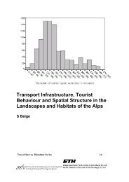
Figure 1 integrates these concepts into an overall decision-tree for a trip-maker’s choice of 

travel mode(s) for a single tour. Note that at the overall home-based tour level two options 

exist: drive chain (D), or non-personal-vehicle chain (NPV). Also note that within the NPV 

chain, trip modes are selected on an individual trip basis. 

Figure 1 

Tour-Level Decision Tree With a Sub-Chain 

Drive Option for Chain c 

Chain c: 

1. Home-Work 

2. Work-Lunch 

3. Lunch-Meeting 

4. Meeting-Work 

5. Work-Home 

NPV Option for Chain c 

Drive for 

Sub-chain s 

m1 = drive 

Sub-Chain s: 

2. Work-Lunch 

3. Lunch-Meeting 

4. Meeting-Work 

NPV for 

Sub-chain s 

m1 m2 m3 

m4 m5 

mN = mode chosen for trip N 

m2 = drive 

m3 = drive 

m4 = drive 

m5 = drive 

m2 

m3 m4 

6


August 10-15, 2003 

A random utility approach is adopted in this model to determine the choice among these options. 

The utility of person p choosing mode m for trip t on trip chain c, U(m,t,p), is: 

U(m,t,p) = V(m,t,p) + ε(m,t,p) t∈T(c,p); m∈f(t,p) [1] 

where: 

V(m,t,p)= 

ε(m,t,p)= 

T(c,p) = 

f(t,p) = 

systematic utility component of mode m for trip t for person p 

random utility component of mode m for trip t for person p 

set of trips on chain c for person p 

set of feasible modes for trip t for person p 

Further, we assume that the utility for a specific combination of chosen modes for the entire 

trip chain c, U(M,p) is simply the sum of the individual trip utilities: 

U(M,p) = ∑ t∈T(c,p) V(m(t),t,p) + ∑ t∈T(c,p) ε(m(t),t,p) M∈F(c,p) [2] 

where: 

M = one set of specific feasible modes for the trips on chain c for person p (the 

chain mode set) 

F(c,p) = set of chain mode sets for chain c for person p; this set is defined by both a 

priori trip constraints (e.g., trip distance too long to walk) and chain-based “contextual” 

constraints (e.g., can’t use auto-drive on return trip if it was not used on the outbound 

trip) 

A special case of M is the all-drive chain (D), for which equation [2] simplifies to: 

U(D,p) = ∑ t∈T(c,p) V(d,t,p) + ∑ t∈T(c,p) ε(d,t,p) [3] 

where d represents the drive trip mode. 

The other values of M involve the feasible combinations of individual trip-based mode 

choices (e.g., for a three-trip tour: transit-transit-transit; transit-walk-taxi; etc.) that define the 

NPV chain option. Since in the case of the NPV option the mode for each trip in the chain is 

chosen individually, equation [2] reduces to: 

U(NPV,p) = ∑ t∈T(c,p) MAX m∈f(t,p) [U(m,t,p)] [4] 

where U(NPV,p) is the optimal NPV chain mode set. 

Equation [2] represents a major assumption in the model design. It is essential to provide a 

consistent comparison between chain-based and trip-based modes, as well as to deal with 

7


August 10-15, 2003 

ride-sharing and joint-travel mode choices. Note that this is effectively the standard assumption 

implicit in trip-based models. 

The standard random utility assumption is made that the chain mode set chosen is M* for 

which: 

U(M*,p) ≥ U(M,p) ∀ M,M* ∈ F(c,p); M* ≠ M [5] 

That is, the D or (optimal) NPV chain mode set will be chosen for the given trip chain, depending 

on which provides the maximum utility to the trip-maker. 

As with any random utility model, the selection of the probability distribution for the error 

terms, ε(m,t,p), represents a critical step in the model specification. In most discrete choice 

models, criterion [5] would be integrated over the selected error distribution to yield the probability 

that person p would choose chain mode set M*; that is to compute: 

P(M*,p) = Prob[U(M*,p) ≥ U(M,p) ∀ M,M* ∈ F(c,p); M* ≠ M] [6] 

The error distribution is usually selected to facilitate the calculation of equation [6], which 

typically means the assumption of some form of either a generalized extreme value (GEV) 

distribution or a mixed logit representation, where the selection among these competing functional 

forms is driven by considerations of an appropriate covariance structure for the ε’s. 

Unfortunately, the model presented in equations [1]-[5] does not “fit” well within these standard 

functional forms. In particular, the non-personal-vehicle decision structure is nonstandard 

in that the overall chain mode set choice depends upon the sum of a set of individual 

trip mode choices. This does not translate directly into a GEV framework. 

In our model, we choose to forego the need for equation [6] altogether and, instead, work directly 

at the level of equation [5]. That is, given an assumed probability distribution for the 

ε’s, we generate a set of ε(m,t,p) for each mode and trip for each person p and evaluate criterion 

[5] directly. The chain mode set M* that receives the highest utility score is then simply 

selected. If P(M*,p) is required (e.g., for parameter estimation purposes), then this process is 

simply replicated with many independent random draws in order to simulate P(M*,p) by the 

frequency with which M* is selected. 

While recognizing that a certain computational burden is inherent in this approach (along with 

some estimation issues, see Section 7), it also brings with it several potentially interesting and 

important advantages. These include: 

• The modeller is free to use any probability distribution for the error terms that makes 

theoretical sense and is empirically supported by the data, rather than having to assume 

a distribution that is analytically tractable. 

• The approach exploits the Monte Carlo simulation framework to work directly at the 

behaviourally more fundamental level of the random utility, rather than having do go 

through the intermediate process of synthesizing choice probabilities 

8


August 10-15, 2003 

• Working directly at the level of the random utilities allows for very complex choice 

structures to be constructed in a computationally efficient, theoretically plausible way, 

without the need to construct increasingly unwieldy “nesting” structures. 

In this model, we choose to assume that the errors are normally distributed. The two obvious 

advantages of this assumption are: 

• when trip errors are added together in equation [2] to compute chain-level utilities, this 

utility remains normally distributed; and 

• very general covariance structures for the joint error distribution are supported by the 

multivariate normal distribution. 

4.3 Vehicle Allocation 

To this point it has been assumed that any valid driver can choose the drive mode chain option 

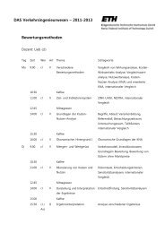
if he/she so wishes. It is possible, however, for conflicts to occur in which two or more 

potential drivers within a household wish to use the same vehicle at the same time. Figure 2 

illustrates this situation for the simple but relatively common case of a two-driver, one-vehicle 

household. In such cases, a conflict resolution mechanism is required to determine which 

driver(s) actually get to use the household’s vehicle(s). 

Figure 2 

Vehicle Allocation: 2-Driver, 1-Vehicle Case 

Person 1 Person 2 Car 1 

Time 

Request for 

car 

Allocation of 

the car to a 

given person 

9


August 10-15, 2003 

Let ndr(τ) be the number of household trip-makers who wish to use a household vehicle at 

time τ. Let nveh be the number of vehicles available for the household’s use. If the condition 

holds that: 

ncar ≥ ndr(τ) [7] 

then all drivers are free to use a car on their tour. If, however, condition [7] is not true, then 

(ndr(τ)-ncar) trip-makers must use their “second best” chain mode option. 

In this model the assumption is that this decision is made so as to maximize total household 

utility, which is defined as the sum of the utilities of the individual household trip-makers. 

This is equivalent to maximizing: 

Σ p [U(D,p) – U(NPV,p)]x p [8] 

subject to: Σ p x p = ncars [9] 

where: 

x p = 1 if person p is allocated a car; = 0 otherwise. 

Cases may well occur in which a “second best”, non-drive option does not exist for a given 

trip-maker. In such cases, U(NPV,p) is currently simply set to a very large negative number 

so that expression [8] can still be evaluated. 2 If such a person’s request for a car is rejected, 

then two further options exist: 

1. The person may attempt to reschedule the activities on the rejected tour for another 

time period when a car will be available. This process lies outside of the mode choice 

model being discussed here. 

2. The household can investigate options for ride-sharing between the “accepted” and 

“rejected” drivers (see below). 

4.4 Serve-Passenger/Auto-Passenger Modes 

Auto-passenger trips occur in three ways: 

1. shared-ride in a joint activity; 

2. passenger in an inter-household "car-pool"; and 

3. passenger being “chauffeured” in a car driven by another household member. 

2 

This suffices for present model estimation purposes, but it is not the ideal solution. It would be better to 

measure the actual “utility loss” associated with foregoing the trip chain. This is beyond the current capability 

of the prototype model, but is an area for future research. 

10


August 10-15, 2003 

Since each of these activities is complex and involves the interaction with at least one other 

person, it is argued that the auto-passenger mode should be determined as an inter-personal 

decision process and should not be included in the individual person tour mode choice model 

that has been presented above. Joint activity mode choice is discussed below. Interhousehold 

car-pooling is an extremely difficult process to represent, and is not addressed 

within the current model. 

Serve-passenger trips are determined in a “second-pass” procedure. That is, when a new activity 

episode is being inserted into a schedule (and, hence, a trip chain), auto-passenger is not 

considered as a mode for the new travel episodes involved. Utilities are calculated based on 

the other feasible modes, provisional mode choices are made, and vehicle allocations are 

sorted out, as has been described above. Subsequently, auto-passenger options for nondrivers 

are assessed. 

The basic logic of the serve-passenger decision is that if overall household utility can be improved 

through the ride-share and the ride-share is feasible (given the driver’s schedule), then 

it is “worth” doing. For this to happen the “utility gain” of the passenger must exceed the 

“utility loss” of the driver. Note that even if two people are driving, opportunities for ridesharing 

may still exist (i.e., substituting auto-passenger for auto-drive for one of the drivers 

and a SOV-drive for a rideshare-drive for the other), if the utility gain for the household is 

sufficient. 

Intra-household ride-sharing has not yet been implemented within the model prototype. For 

present purposes, the key point to note is that it is clear that the utility-based microsimulation 

modelling approach proposed in this paper is extensible to dealing with inter-personal, withinhousehold 

ride-share tradeoffs in a way that traditional probability-based models would have 

difficulty undertaking. 

4.5 Joint Travel 

Joint activities are household-level projects involving two or more household members. 

Mode choice for joint activities should be handled the same as for individual trips, except: 

• Mode choice is now a joint decision, simultaneously determined for all joint activity 

participants. 

• Auto-drive is replaced by shared-ride. That is, the model will not attempt to determine 

who drives and who is a passenger. 

To be consistent with the individual trip model, total travel times and travel costs must be 

computed by adding the travel times and costs of all joint trip members. Not only is this required 

to maintain a consistent treatment of trip utilities throughout the model, but it facilitates 

dealing with “mixed” individual-joint tours. 

Joint tours can occur in two ways. The more common is a “pure” joint tour, in which the 

11


August 10-15, 2003 

members of the joint party travel together throughout the tour. “Mixed” tours, in which one 

or more trips made by one or more of the joint activity members are made independently, 

however, are also certainly feasible. In such cases, equation [2] “simply” extends to assess 

the combined utility of all trips of the two (or more) trip-chains that are “linked” by the joint 

activities. That is, while the complexity of keeping track of the modal options across the 

linked tours clearly increases, conceptually the procedure remains the same as for the individual 

tour case. 

5. Prototype Implementation 

The conceptual model described above has been estimated in a prototype formulation. As has 

been discussed, this prototype does not deal with the auto passenger mode (either through intra-household 

ride-sharing or inter-household car-pooling), nor does it include joint activity 

chains. Further, to keep the initial model as simple as possible, only tours including the “primary 

modes” of auto-drive, transit (with walk access) and walk all-way are included. Otherwise, 

however, it represents a full implementation of the conceptual model, including the 

“dynamic” vehicle allocation among competing drivers. 

As noted above, the assumption of normally distributed random terms allows for a very generalized 

covariance structure. In order to exploit this generality somewhat in the current investigation, 

while keeping this preliminary analysis reasonably simple, the following error 

structure has been assumed: 

ε(m,t,p) = µ(m,p) + η(m,t,p) [10] 

where: 

µ(m,p) ≈ MVN(0,Σ) ∀ p [11] 

η(m,t,p) ≈ N(0,σ) ∀ m,t,p [12] 

That is, µ is a mode-specific error term that captures person p’s idiosyncratic taste variation 

for mode m, relative to the population average preference. In the simplest model tested, µ is 

assumed to be iid (i.e., once scaled for identification purposes, Σ is simply the identity matrix), 

but a heteroscedastic (non-equal diagonal terms) model is also estimated. 

On the other hand, η is a “pure random” effect that varies from mode to mode within a trip 

and from trip to trip. 

While in principle the two error terms could be added together (since they are both normally 

distributed), it is essential to keep them separate so as to be able to identify the “fixed” modespecific 

component relative to the “variable” trip-specific component. This model is analogous 

to a mixed logit model in which normally distributed alternative-specific bias parameters 

are imbedded within a logit kernel. Statistical identification criteria for the model are discussed 

in Appendix A. 

12


August 10-15, 2003 

Finally, while not required by either the conceptual model’s assumptions our for computational 

convenience, the operational prototype makes the standard assumption that the systematic 

utility function is linear in the parameters. 

6. Data 

The data used to estimate the prototype model parameter values are taken from the 1996 

Transportation Tomorrow Survey (TTS). TTS is a one-day, telephone-based, travel survey of 

5% of households within the Greater Toronto Area (GTA) that was undertaken in the autumn 

of 1996 (DMG, 1997). In the survey, all trips made by all surveyed household members 11 

years of age or older were recorded for a randomly selected weekday, along with household 

socio-economic information. This trip-based dataset was converted into a set of out-of-home 

activities and trip-chains by Eberhard (2002). 

Table 1 

1996 TTS Total Sample & Estimation Sub-Sample Summary Statistics 

TTS 

Estimation Sample 

TTS Total 

Households 

(Raw) 

TTS Trip 

making 

households 

(cleaned) 

No carpool / 

rideshare / joint 

activities 

Total 

Final Estimation 

Set 1 

Households 88898 68538 41981 4000 3511 

Persons 243286 192960 106276 10177 5684 

2 

Trip Chains N/A 176041 80627 7712 6490 

Trips 500313 405809 180731 17238 14570 

Drive 3 311502 62.3% 251530 62.0% 122848 68.0% 11479 66.6% 10233 70.2% 

Drive Acc Subway 863 0.2% 648 0.2% 395 0.2% 29 0.2% 0 0.0% 

Drive Egr Subway 798 0.2% 609 0.2% 376 0.2% 28 0.2% 0 0.0% 

Drive Acc Go Rail 1241 0.2% 910 0.2% 649 0.4% 74 0.4% 0 0.0% 

Drive Egr Go Rail 1161 0.2% 862 0.2% 630 0.3% 72 0.4% 0 0.0% 

Non-drive Go Rail 4 2216 0.4% 1609 0.4% 878 0.5% 64 0.4% 0 0.0% 

Transit All-way 59760 11.9% 50793 12.5% 33932 18.8% 3442 20.0% 3135 21.5% 

Walk 29250 5.8% 24813 6.1% 14413 8.0% 1414 8.2% 1202 8.2% 

Taxi 2386 0.5% 1866 0.5% 1058 0.6% 107 0.6% 0 0.0% 

Schoolbus 7684 1.5% 6322 1.6% 3112 1.7% 305 1.8% 0 0.0% 

Bicycle 3891 0.8% 3349 0.8% 2440 1.4% 224 1.3% 0 0.0% 

Passenger 78768 15.7% 62311 15.4% 0 0.0% 0 0.0% 0 0.0% 

Other/Unknown 793 0.2% 187 0.0% 0 0.0% 0 0.0% 0 0.0% 

Notes: 

(1) Trips by modelled modes complying with all choice set rules. 

(2) Only includes persons making a trip. Other columns include all persons in the households. 

(3) Drive includes motorcycle trips. 

(4) “GO Rail” is the GTA commuter rail system. “Non-drive GO” indicates transit, walk, 

auto passenger and taxi commuter rail station access modes. 

13


August 10-15, 2003 

Table 1 provides summary statistics on the full TTS dataset, the total set of households for 

which “cleaned” sets of activities and tours were successfully constructed by Eberhard, and 

the subset of households which did not engage in car-pool, ride-share or joint activities (the 

target population for the prototype model). In order to keep model estimation computations 

within reasonable limits, a 4,000 household random sample was drawn from the 41,981 total 

households in this last category. This random sample reflects the larger group’s trip mode 

distribution very well. Also note that the auto-drive, transit all-way and walk modes account 

for 94.8% of the estimation sample trips. The commuter rail and subway drive access modes 

were excluded from the prototype model due to the very small number of trips made by these 

modes, while taxi, school-bus and bicycle trips were eliminated due to unavailability of suitable 

explanatory variables with which to construct modal utility functions. The end result is a 

final estimation dataset consisting of 3,511 households, 5,684 persons who executed at least 

one trip chain, 6,490 trip chains and 14,570 individual trips. 

All auto and transit travel times and costs were obtained from EMME/2-based network calculations 

performed within the GTAModel regional travel demand modelling system for the 

GTA. 3 Walk travel times were estimated based on simple straight-line origin to destination 

travel distances and assumed average travel speeds. 

7. Parameter Estimation Procedure 

Model parameter values were estimated by maximizing the log-likelihood function: 

L(β) = Σ h Σ p∈H(h) Σ c0C(p) Σ t0T(c,p) log(P(m*,t,p|β)) [13] 

where: 

H(h) = set of persons 11 years or older in household h 

C(p) = set of home-based tours for person p 

β = vector of model parameters (including parameters of the error distribution) to 

be estimated 

P(m*,t,p|β) = simulated probability of person p choosing the observed mode m* for trip t on 

chain c, given the model parameters β. 

P is simulated through a Monte Carlo process in which N sets of random utilities U are drawn 

for each trip for each person for each chain for a given β, equation [5] is evaluated for each 

draw, and the frequency with which m* is predicted to be chosen is accumulated. In order to 

3 

For EMME/2 documentation see Inro (1999). For GTAModel documentation see Miller (2001). 

14


August 10-15, 2003 

account for the possibility that m* is never chosen within the N draws, P is defined as (Ortuzar 

and Willumsen, 2001): 

P(m*,t,p|β) = [F(m*,t,p|β) + 1] / [N + n t ] [14] 

where F(m*,t,p|β) is the number of times m* was selected for trip t out of the N draws, and n t 

is the number of feasible modes for trip t. 

Since log(P) is not analytically defined, standard gradient-based methods for optimizing [13] 

are not directly applicable (cf. Train, 2002). In this application a very simplistic random 

search procedure was used in which a large number of random parameter sets were generated, 

and L(β) was evaluated at each of the randomly generated values of β. The search area was 

systematically reduced in a series of stages, centred upon the best parameter set found in each 

search stage. Although time-consuming and computationally intensive, the procedure appears 

to yield stable results. In particular, given the evaluation of a wide variety of parameter values 

over an (initially) extensive domain, local optima did not pose a discernible problem, and 

we are quite confident that the procedure is converging on the global maximum. 

Alternative (and probably smarter!) estimation procedures that should be investigated include 

using a genetic algorithm to focus the random search, and/or trying to fit a surface to the randomly 

generated points so that a quasi-gradient can be computed that might permit some form 

of hill-climbing procedure to be locally applied. A more detailed discussion of the estimation 

procedure used in this model, in comparison with other methods, will be presented in a forthcoming 

paper by the authors. 

8. Model Estimation Results 

Results for two estimated models are presented in this paper. The first is an iid model in 

which the variance of µ(m,p) is normalized to 1 for all m. The second model has the same 

systematic utility specification as Model 1, but has individual variance terms for µ for each 

mode m (with the variance for the auto-drive term being normalized to 1.0). Table 2 defines 

the variables included in both models. The utility functions employed are relatively simple in 

structure and could, of course, be further elaborated. Points to note concerning this specification 

include the following. 

• Travel times and costs are generic across modes, with the exception of auto and transit 

in-vehicle travel times, which have alternative-specific parameters. 

• The aggregate zone-to-zone transit assignment used to generate transit travel times 

does not generate in-vehicle travel times for intrazonal and adjacent zone trips. While 

travel times for these trips were estimated based on origin-to-destination trip distances, 

the intrazonal and adjzone dummy variables were included in the model specification 

to account for possible biases in these measurements, as well as to capture the possible 

systematic disutility of using transit for very short trips. 

15


August 10-15, 2003 

• The Toronto central area (often designated “Planning District 1”) is much denser and 

more conducive to walking than other areas within the GTA. The dest_pd1 dummy is 

intended to capture systematic preferences for walking within this district. 

Table 2 

Definition of Explanatory Variables 

Parameter Description 

c-tr_n_dr Mode specific constant for transit all-way 

c-walk Mode specific constant for walk 

atime Auto in-vehicle travel time (min) 

tivtt 

Transit in-vehicle travel time (min) 

walktt Walk travel time including walk access to/from transit (min) 

twait Transit wait time (min) 

travelcost Travel cost ($1996) 

pkcost Parking cost ($1996) 

dpurp_shop =1 if trip purpose = shopping (auto mode); = 0 otherwise 

dpurp_sch =1 if trip purpose = school (auto mode); = 0 otherwise 

dpurp_oth =1 if trip purpose = other (auto mode); = 0 otherwise 

dest_pd1 =1 for walk trips destined for downtown Toronto; = 0 otherwise 

intrazonal =1 for an intrazonal trip for the transit all-way mode; = 0 otherwise 

adjzone =1 for an adjacent zone for the transit all-way mode; = 0 otherwise 

Etrip_par (σ/s d ) Scaled variance for the trip specific error η pmt 

Covar2 (s t /s d ) Scaled variance of the mode specific error term (transit all-way mode) 

Covar3 (s w /s d ) Scaled variance of the mode specific error term (walk mode) 

Variable Average Std.Dev. Variable Average Std.Dev. 

atime 13.1 11.4 dpurp_shop 0.155 0.361 

tivtt 26.3 22.4 dpurp_sch 0.046 0.210 

twalk 21.5 21.3 dpurp_oth 0.241 0.428 

twait 7.1 4.9 dest_pd1 0.102 0.303 

cost 1.7 1.5 intrazonal 0.071 0.257 

parkcost 0.75 1.96 adjzone 0.029 0.167 

Table 3 presents parameter estimates and goodness-of-fit statistics for both models. Asymptotic 

t-statistics are not available for these estimates at this time, due to difficulties encountered 

in numerically computing the log-likelihood Hessian function in the absence of an analytical 

log-likelihood function. It is expected that these problems will be resolved by the time 

the paper is presented at the conference in August, and that t-statistics will be added to Table 

3 at that time. 

16


August 10-15, 2003 

Table 3 Model Estimation Results 

Parameter Model 1 Model 2 

c-tr_n_dr -1.3233 -1.1539 

c-walk 0.4977 0.0805 

atime -0.2958 -0.3553 

tivtt -0.0963 -0.1086 

walktt -0.4366 -0.5629 

twait -0.8383 -1.2279 

travelcost -0.0862 -1.0241 

pkcost -2.2220 -3.0333 

dpurp_shop 4.5812 3.6322 

dpurp_sch 0.1364 0.0909 

dpurp_oth 3.8700 6.7735 

dest_pd1 3.2801 4.6257 

intrazonal -9.8869 -12.7177 

adjzone -6.5433 -8.1285 

CovarIndex1 1 1 

CovarIndex2 6.6803 

CovarIndex3 0.3508 

Etrip_par 6.4217 6.5675 

Num Observations 14570 14570 

Num Parameters 16 18 

Log Lik Max L(beta) -4184.4 -4186.7 

Log Lik No Param L(0) -9486.9 -9486.9 

-2[L(0)-L(beta)] 10605 10600.3 

rho2 0.5589 0.5587 

Adjusted rho2 0.5572 0.5568 

Obs. Mode Never Chosen 28 45 

Note: CovarIndexN is the variance parameter for auto (1), transit (2) and walk (3). The auto variance is normalized 

to 1 in all models. 

Points to note from Table 3 include the following. 

• All parameters have expected signs. 

17


August 10-15, 2003 

• All parameters are of plausible magnitude, except the travelcost parameter in Model 1, 

which, combined with the parameter values for atime and tivtt, implies values of time 

of $205/hr for auto users and $67/hr for transit users. Model 2 returns much more reasonable 

values of time of $21/hr and $6.4/hr for auto and transit users, respectively, 

which are generally consistent with other values of time obtained in GTA travel demand 

models. 

• Both models fit the data very well and produce virtually the same overall goodness of 

fit (an adjusted ρ 2 of 0.557 in both cases). 

• Despite the same overall fit, the heteroscedastic Model 2 generally yields more plausible 

parameter estimates. In addition to the improved time and cost parameters already 

discussed, the walk alternative-specific constant is much smaller in magnitude in 

Model 2 (and may well be insignificant), and the dpurp_sch dummy variable (for 

which a strong a priori hypothesis does not exist) is very small in magnitude (and almost 

certainly insignificant) in Model 2. 

• The random trip error term (η) possesses a very strong variance parameter (Etrip_par) 

in both models, which suggests that the trip-specific component of the error structure 

is significantly different from the mode-specific component. 

• The heteroscedastic variance parameters for transit and walk are almost certainly significantly 

different from one, and hence significantly different from the auto variance 

term. The fact that the transit variance is much larger than auto-drive (and of the same 

order of magnitude as the individual trip variance) is plausible, as is the much smaller 

walk variance. 

• An important concern in simulated log-likelihood calculations is the possibility that an 

observed mode for a given observation is never chosen within the Monte Carlo simulation. 

In this analysis, 100 random draws were generated per trip. As shown in Table 

2, only 28 of the 14,570 trips (0.19%) did not have the observed chosen mode selected 

at least once during the Model 1 simulation, while observed modes where never selected 

for 45 trips (0.31%) in Model 2. While ideally this number should be driven to 

zero as the estimation proceeds, such a very small number of “never chosen” trips is 

not likely to be having a large impact on the model estimation results. 

Table 4 presents prediction-success tables for both models. Again, the good fit of both 

models is indicated in this table, with almost 89% of observed modes being chosen on average. 

In addition, each mode is well predicted with prediction success rates in the order 

of 95%, 75% and 70% for the auto-drive, transit and walk modes, respectively. Relatively 

little “confusion” exists within the model, with off-diagonal elements being generally 

small and “well balanced” (approximately as many transit trips are incorrectly assigned to 

walk as walk trips are assigned to transit, and so on). 

Finally, note in Table 4 that the aggregate predicted mode shares very closely match the 

observed mode shares. Unlike a conventional logit model estimation procedure, for 

18


August 10-15, 2003 

Table 4 Prediction-Success Tables for the Estimated Models 

Model 1: IID Error Terms 

(a) Trips 

Predicted Mode 

Obs.Mode Drive Walk Transit Total 

Drive 9698.21 385.73 149.06 10233 

Transit 514.69 2399.93 220.38 3135 

Walk 104.62 270.98 826.4 1202 

Total 10317.52 3056.64 1195.84 14570 

% of Total Trips Predicted Mode 


Drive 66.6% 2.6% 1.0% 70.2% 

Transit 3.5% 16.5% 1.5% 21.5% 

Walk 0.7% 1.9% 5.7% 8.2% 

Total 70.8% 21.0% 8.2% 100.0% 

% of Obs. Mode Predicted Mode 


Drive 94.8% 3.8% 1.5% 100.0% 

Transit 16.4% 76.6% 7.0% 100.0% 

Walk 8.7% 22.5% 68.8% 100.0% 

Total 70.8% 21.0% 8.2% 100.0% 

Model 2: Heteroscedastic Error Terms 

(a) Trips 

Predicted Mode 


Drive 9740.5 386.08 106.42 10233 

Transit 519.76 2378.17 237.07 3135 

Walk 108.25 248.75 845 1202 

Total 10368.51 3013 1188.49 14570 

% of Total Trips Predicted Mode 


Drive 66.9% 2.6% 0.7% 70.2% 

Transit 3.6% 16.3% 1.6% 21.5% 

Walk 0.7% 1.7% 5.8% 8.2% 

Total 71.2% 20.7% 8.2% 100.0% 

% of Obs. Mode Predicted Mode 


Drive 95.2% 3.8% 1.0% 100.0% 

Transit 16.6% 75.9% 7.6% 100.0% 

Walk 9.0% 20.7% 70.3% 100.0% 

Total 71.2% 20.7% 8.2% 100.0% 

19


August 10-15, 2003 

example, in which predicted and observed mode shares are forced to match through the selection 

of the alternative-specific parameter values, no such constraint is imposed within this 

model’s estimation. Thus, the ability to reproduce the observed shares is a reasonably strong 

test of the model’s overall performance. 

Clearly, given the preliminary nature of the model estimations undertaken to date (along with 

the current absence of parameter asymptotic t-statistics), these results are suggestive, rather 

than in any way definitive, in nature. Nevertheless, it is argued that the results are encouraging 

as tentative indicators of the credibility and practicality of the proposed model. 

9. Conclusions & Future Work 

The model presented in this paper is a “hybrid”, in which rules are combined with a “classical” 

random utility maximization decision criterion within an explicit microsimulation 

framework to model tour-level mode choices. The microsimulation framework is critical to 

the model’s functioning, since it permits decisions to be based directly on simulated utilities, 

thereby avoiding the need to express the choice process in an analytically (or at least computationally) 

tractable choice probability expression. Through this approach, complex personal 

and inter-personal decisions can be modelled in a very tractable manner. In particular, note 

that additional modes and “decision levels” (e.g., vehicle allocation, serve-passenger, etc.) can 

be added to the model with minimal additional model complexity (albeit with inevitable additional 

computational requirements). This can be contrasted with a “conventional” nested logit 

approach, for example, in which the combinatorics of additional modes and/or decision levels 

quickly render the model computationally cumbersome. 

In order to reduce nested logit combinatorics, current models tend to make strong simplifying 

assumptions, such as first choosing a “primary mode” for the tour, restricting the number of 

“secondary” modes considered for a tour, and /or restricting the size/complexity of tours that 

are considered within the model. They also do not deal explicitly with inter-personal decision-making 

associated with auto-passenger trips and joint activities. In the model presented 

above none of these limitations is inherent in the model structure: no a priori judgements 

concerning “primary” modes are required; tours of any level of complexity are supported 

within the model; and the model is explicitly designed to deal with inter-personal decisionmaking. 

Further, the model structure imposes no a priori constraints on the random utility error structure 

that can be assumed. Given this, normally distributed error terms are used, due to the 

flexible and generally attractive features of the normal distribution, plus the practical usefulness 

of being able to add trip-level errors to yield chain-level errors that possess the same distribution 

type. 

These model strengths, of course, do not come without some cost. The computational burden 

of performing many replications of the choices so as to achieve statistically representative 

outcomes is non-trivial. Also, as has been discussed, statistical estimation of the model’s pa- 

20


August 10-15, 2003 

rameters is an onerous task and requires the use of special procedures, with much more work 

in this area being required before a “standard” procedure can be said to exist. Given, however, 

that the result is the ability to model tour-based travel for all trips made by all household 

members over an entire twenty-four hour period in an internally self-consistent and theoretically 

credible manner, it is argued that these are costs well worth paying. 

Clearly, much work remains in terms of the conceptual and operational elaboration of this 

model. The operational model must be extended to include within-household ride-sharing, 

joint activity chains, and a wider variety of travel modes (e.g., bicycle, taxi, commuter rail). 

Considerably more development and testing of the parameter estimation procedure is required. 

The model needs to be tested with more detailed activity-based data. It needs to be 

integrated with the TASHA activity scheduler provide “dynamic” mode selections as part of 

the daily scheduling process. And, finally, it is hoped that the utility-based, microsimulation, 

household-based modelling approach (of which this tour-based mode choice model is a specific 

instance) can be extended to provide an integrated, comprehensive model of household 

short- and long-run decision-making (Miller, 2003). 

10. REFERENCES 

Algers, S., A.J. Daly, and S. Widlert (1997) Modelling travel behaviour to support policy 

making in Stockholm, P. Stopher and M. Lee-Gosselin (eds.), Understanding Travel 

Behaviour in an Era of Change. Oxford: Pergamon. 

Arentze, T. and H. Timmermans (2000) ALBATROSS: A Learning Based Transportation 

Oriented Simulation System, Den Haag: European Institute of Retailing and Services 

Studies. 

Asensio, J. (2002) Transport mode choice by commuters to Barcelona’s CBD, Urban Studies 

39(10), 1881–1895. 

Ben-Akiva, M., D. Bolduc, and J. Walker (2001) Specification, Identification, and Estimation 

of the Logit Kernel (or Continuous Mixed Logit) Model, Working Paper, Cambridge 

MA: Department of Civil & Environmental Engineering, MIT. 

Ben-Akiva, M., J. Bowman, S. Ramming and J. Walker (1998) Behavioral Realism in Urban 

Transportation Planning Models, in Transportation Models in the Policy-Making 

Process: A Symposium in Memory of Greig Harvey. Asilomar Conference Center, California. 

Beser, M. and S. Algers (2002) SAMPERS - The New Swedish National Travel Demand 

Forecasting Tool, in L. Lundqvist and L-G. Mattsson (eds.) National Transport Models: 

Recent Developments and Prospects, Stockholm: Springer. 

Bowman, J., M. Bradley, Y. Shiftan, T. K. Lawton and M. Ben-Akiva (1998) Demonstration 

of an Activity Based Model System for Portland," in 8 th World Conference on Transport 

Research, July 12-17, Antwerp. 

Bowman, J. and M. Ben-Akiva (2000) Activity-based Disaggregate Travel Demand Model 

System with Activity Schedules," Transportation Research A, 35, 1-28. 

21


August 10-15, 2003 

Bradley, M., M. L. Outwater, N. Jonnalagadda and E.R. Ruiter (2001) Estimation of Activity- 

Based Mocrosimulation Model for San Francisco, in Proceedings of the 80 th Annual 

Meeting of the Transportation Research Board, Washington D.C. 

Bunch, D (1991) Estimability in the Multinomial Probit Model, Transportation Research B, 

25, 1-12. 

Cascetta, E., A. Nuzzolo, and V. Velardi (1993) A System of Mathematical Models for the 

Evaluation of Integrated Traffic Planning and Control Policies, Unpublished Research 

Report, Laboratorio Richerche Gestione e Controllo Traffico, Salerno, Italy. 

Cirillo, C. and K. W. Axhausen (2002) Mode choice of complex tours: A panel analysis, in 

Arbeitsberichte Verkehrs- und Raumplanung, 142. Zurich: Institut für Verkehrsplanung, 

Transporttechnik, Strassenund Eisenbahnbau (IVT), ETH Zurich. 

Coleman, J. (2002) An Improved Mode Choice Model for the Greater Toronto Travel 

Demand Modelling System, Research Report, Toronto: Joint Program in 

Transportation. 

DMG (1997) TTS Version 3: Data Guide, Research Report, Toronto: Data Management 

Group, University of Toronto Joint Program in Transportation. 

Eberhard, L. (2002) A 24-Hour Household-Level Activity-Based Travel Demand Model for 

the GTA, MASc thesis, Toronto: Department of Civil Engineering, University of 

Toronto. 

Fosgerau, M. (2002) PETRA - An Activity-based Approach to Travel Demand Analysis, in L. 

Lundqvist and L-G. Mattsson (eds.) National Transport Models: Recent Developments 

and Prospects. Stockholm: Springer. 

Hague Consulting Group (1992) The Netherlands National Model, 1990: The National Model 

System for Traffic and Transport, Ministry of Transport and Public Works, The 

Netherlands. 

INRO (1990) EMME/2 User's Manual, Software Release: 9.0, Montreal: INRO Consultants 

Inc. 

Jonnalagadda, N., J. Freedman, W. A. Davidson, and J. D. Hunt (2001) Development of 

Microsimulation Activity-Based Model for San Francisco: Destination and Mode 

Choice Models, Transportation Research Record, 1777, 25-35. 

Kitamura, R., C. Chen, R. Pendyala, and R. Narayana (2000) Micro-simulation of Daily 

Activity-travel Patterns for Travel Demand Forecasting, Transportation, 27, 25-51. 

Miller, E.J. (2001) The Greater Toronto Area Travel Demand Modelling System, Version 2.0, 

Volume I: Model Overview, Research Report, Toronto: Joint Program in 

Transportation, University of Toronto. 

Miller, E.J. (2003) Propositions for Modelling Household Decision-Making, submitted for 

publication in, M. Lee-Gosselin and S.T. Doherty (eds), Proceedings of the 

International Colloquium on The Behavioural Foundations of Integrated Land-use and 

Transportation Models: Assumptions and New Conceptual Frameworks. 

Miller, E.J. and M.J. Roorda (2003) A Prototype Model of Household Activity/Travel 

Scheduling, forthcoming in Journal of Transportation Research Record. 

22


August 10-15, 2003 

Ortúzar, J. de D. (1983) Nested Logit Models for Mixed-mode Travel in Urban Corridors, 

Transportation Research 17A (4), 283-299. 

Ortúzar, J. de D. and L. Willumsen (2001) Modelling Transport, Chichester NY: Wiley. 

Train, K. (2002) Discrete Choice Methods with Simulation, Cambridge: Cambridge 

University Press, preprint available at http://else.berkeley.edu/books/train1201.pdf. 

Appendix A: Statistical Identification of Model Parameters 

The procedure followed here is inspired by Bunch (1991) and Ben-Akiva, et al., (2001). It 

involves examining whether the model meets order, rank and positive definiteness conditions. 

Recall that the model error structure is: 

ε(m,t,p) = µ(m,p) + η(m,t,p) 

[A.1] 

where: 

µ(m,p) ≈ MVN(0,Σ) 

η(m,t,p)≈ N(0,σ) 

Two cases are considered: 

• a homoscedastic iid model, which has two parameters: one along the diagonal of the 

matrix Σ, and the term σ; and 

• a heteroscedastic, independent model, which has M+1 parameters: M diagonal elements 

in the matrix Σ (where M is the number of trip modes in the model) and the 

term σ. 

The order condition states that a maximum of M(M-1)/2 alternative-specific parameters are 

estimable in Σ. In this case, M = 3; thus, an upper bound on the number of estimable parameters 

in Σ is 3. 

The rank of Σ depends on its specification. In the iid case, the rank of the matrix is 1; in the 

heteroscedastic case, the rank is 3. The “rank” of σ, of course, is 1 for both models. 

The positive definiteness condition is not binding for this model due to its similarities with a 

multinomial probit model, for which any positive normalization is acceptable (Ben-Akiva, et 

al., 2001). 

Finally, the overall utility function U(m,t,p) (equation [1]) is only identified up to scale, resulting 

in a loss of one estimable parameter. Thus, the number of identifiable parameters in 

the model is the sum of the ranks of the two error terms, minus one, to account for the utility 

23


August 10-15, 2003 

function scaling. For the iid model this yields (1+1-1) = 1, while the number of identifiable 

parameters in the heteroscedastic model is (3+1-1) = 3. 

In both models, the variance for the auto-drive error term, µ(d,p), is normalized to 1.0 (thereby 

scaling the overall utility function). In the iid model, this sets Σ equal to the identity matrix. In 

the heteroscedastic model, the other two diagonal elements of Σ are identifiable up to scale (i.e., 

the parameters estimated are the transit over drive and walk over drive variance ratios). In both 

models the variance of η is identifiable up to scale (i.e., the parameter estimated is σ divided by 

the auto-drive variance). 

24

A Tour-Based Model of Travel Mode Choice - Civil Engineering ...

You also want an ePaper? Increase the reach of your titles

Delete template?

Save as template?