Integral Definition of Curl
Integral Definition of Curl
Integral Definition of Curl

You also want an ePaper? Increase the reach of your titles
YUMPU automatically turns print PDFs into web optimized ePapers that Google loves.
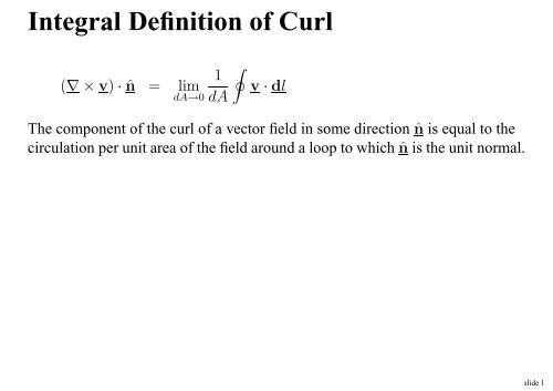
<strong>Integral</strong> <strong>Definition</strong> <strong>of</strong> <strong>Curl</strong><br />
(∇ × v) · ˆn = lim<br />
dA→0<br />
1<br />
dA<br />
∮<br />
v · dl<br />
The component <strong>of</strong> the curl <strong>of</strong> a vector field in some direction ˆn is equal to the<br />
circulation per unit area <strong>of</strong> the field around a loop to which ˆn is the unit normal.<br />
slide 1
Stokes’ Theorem<br />
Divide closed loop C into 2 parts, C1 and C2.<br />
C12<br />
C21<br />
C<br />
C1<br />
Consider the circulation <strong>of</strong> some vector field v around C<br />
∮ ∫ ∫<br />
v · dl = v · dl + v · dl<br />
C<br />
C1 C2<br />
∫ ∫ ∫ ∫<br />
= v · dl + v · dl + v · dl −<br />
∮C1<br />
C12∮<br />
C2<br />
= v · dl + v · dl<br />
C1+C12<br />
C2+C21<br />
C2<br />
C12<br />
v · dl<br />
In other words the contributions from the common curve in each pair <strong>of</strong> loops<br />
cancel.<br />
slide 2
Now consider an open surface S bounded by a curve C. Divide the surface in<br />
to an infinite number <strong>of</strong> infinitesimal rectangles. Add up the circulation <strong>of</strong> v<br />
around all these rectangles.The contribution from all the sides common<br />
between two rectangles i.e. all the sides except those that lay on the curve C,<br />
cancel. This leaves only the contribution from the sides on curve C.So<br />
∮<br />
v · dl = ∑ ∮<br />
v · dl<br />
C i loop i<br />
But for an infinitesimal rectangular loop<br />
∮<br />
loop i<br />
v · dl = (∇ × v) i · ˆn i dA i<br />
ˆn i normal to surface S for loop i (righthand rule) and dA i is the area <strong>of</strong> the<br />
loop.<br />
slide 3
So<br />
∮<br />
C<br />
v · dl = ∑ i<br />
(∇ × v) i · ˆn i dA i<br />
In the limit where the loops are infinitesimal, the sum becomes an integral so<br />
∮ ∫<br />
v · dl = (∇ × v) · ˆn dA<br />
C<br />
Replacing ˆndA with dA, we get<br />
- Stokes’ theorem<br />
Example<br />
S<br />
∮<br />
C<br />
v · dl =<br />
∫<br />
S<br />
(∇ × v) · dA<br />
slide 4
Maxwell’s Equations<br />
Connect one scalar field and three vector fields:<br />
1. ρ = density <strong>of</strong> electric charge (C/m 3 ) - scalar field<br />
2. E = electric field strength - vector field<br />
3. B = magnetic field strength - vector field<br />
4. J = current density (A/m 2 ) - vector field<br />
1 ∇ · E = ρ ǫ 0<br />
2 ∇ · B = 0<br />
3 ∇ × E = − ∂B<br />
∂t<br />
4 ∇ × B = µ 0 J + 1 c 2 ∂E<br />
∂t<br />
slide 5
Faraday’s Law<br />
Electric field induced by a changing magnetic field <strong>of</strong> flux Φ <strong>of</strong> magnetic field<br />
B:<br />
∫<br />
Φ = B · dA - definition<br />
S<br />
− ∂Φ ∮<br />
= E · dl - Faraday’s law<br />
∂t<br />
− ∂ (∫ ) ∮<br />
B · dA = E · dl<br />
∂t S<br />
∮ ∫<br />
E · dl = (∇ × E) · dA<br />
S<br />
∫<br />
× E) · dA = −<br />
S(∇ ∂ (∫ ) ∫<br />
∂B<br />
B · dA = −<br />
∂t S<br />
S ∂t · dA<br />
But this is true for any surface, so<br />
∇ × E = − ∂B<br />
∂t - Maxwell 3<br />
slide 6
Ampère’s Law<br />
Magnetic field B due to a current I<br />
∮<br />
B · dl = µ 0 I<br />
C<br />
where the path C encloses the current I = ∫ s J · dA.<br />
Apply Stokes’ theorem<br />
∫<br />
∮<br />
B · dl =<br />
∫<br />
C<br />
S<br />
∫<br />
(∇ × B) · dA = µ 0<br />
S<br />
S<br />
- must be true for any surface, so<br />
∇ × B = µ 0 J<br />
(∇ × B) · dA<br />
J · dA<br />
This isn’t Maxwell 4 - here the current is time independent.<br />
slide 7
But ...<br />
Can’t be true in general. To see why take the divergence <strong>of</strong> this equation -<br />
∇ · (∇ × B) = 0 - for any B<br />
so ∇ · J = 0<br />
Not in general true. True only for time independent current.<br />
Try<br />
∇ × B = µ 0 J + ǫ 0 µ 0<br />
∂E<br />
∂t<br />
- take the divergence<br />
∇ · (∇ × B) = ∇ · (µ 0 J + ǫ 0 µ 0<br />
∂E<br />
∂t )<br />
but since ∇ · E = ρ ǫ 0<br />
0 = ∇ · J + ǫ 0<br />
∂<br />
∂t ∇ · E<br />
∇ · J + ∂ρ<br />
∂t<br />
= 0 - charge continuity equation<br />
slide 8
Maxwell’s Equations<br />
1 ∇ · E = ρ ǫ 0<br />
⇐⇒ Gauss’ law<br />
2 ∇ · B = 0 ⇐⇒ No magnetic charges<br />
3 ∇ × E = − ∂B ⇐⇒ Faraday’s Law<br />
∂t<br />
4 ∇ × B = µ 0 J + 1 ∂E<br />
⇐⇒ Ampère’s Law<br />
c 2 ∂t<br />
slide 9
EM Waves<br />
Can use Maxwell equations to derive wave equation for em waves.Assume free<br />
space and no current.<br />
∇ × E = − ∂B<br />
∂t<br />
∂E<br />
∇ × B = ǫ 0 µ 0<br />
∂t<br />
Take curl<br />
∂∇ × E<br />
∇ × (∇ × B) = ǫ 0 µ 0<br />
∂t<br />
∇(∇ · B) − ∇ 2 ∂ 2 B<br />
B = −ǫ 0 µ 0<br />
∂t 2<br />
∇ 2 B =<br />
1 ∂ 2 B<br />
c 2 ∂t 2<br />
= −ǫ 0 µ 0<br />
∂ 2 B<br />
∂t 2<br />
where c = 1/ √ ǫ 0 µ 0 - The wave equation for EM waves.<br />
slide 10