HW1_VT13 - KTH

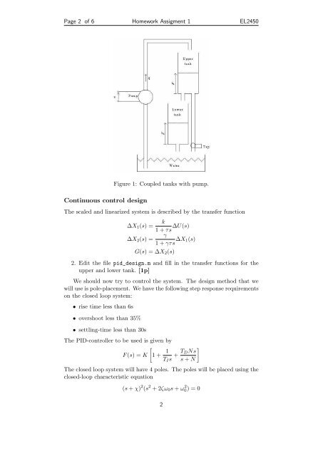
Page 2 of 6 Homework Assigment 1 EL2450
Continuous control design
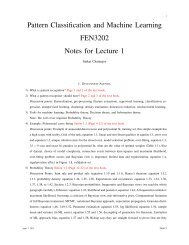
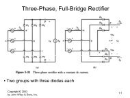
Figure 1: Coupled tanks with pump.
The scaled and linearized system is described by the transfer function
∆X 1 (s) =
k
1 + τs ∆U(s)
γ
∆X 2 (s) =
1 + γτs ∆X 1(s)
G(s) = ∆X 2 (s)
2. Edit the file pid_design.m and fill in the transfer functions for the
upper and lower tank. [1p]
We should now try to control the system. The design method that we
will use is pole-placement. We have the following step response requirements
on the closed loop system:
• rise time less than 6s
• overshoot less than 35%
• settling-time less than 30s
The PID-controller to be used is given by
[
F (s) = K 1 + 1
T I s + T ]
DNs
s + N
The closed loop system will have 4 poles. The poles will be placed using the
closed-loop characteristic equation
(s + χ) 2 (s 2 + 2ζω 0 s + ω 2 0) = 0
2