HW1_VT13 - KTH

EL2450: Hybrid and Embedded Control
Systems: Homework 1
[To be handed in February 8]
Introduction
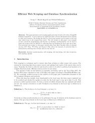
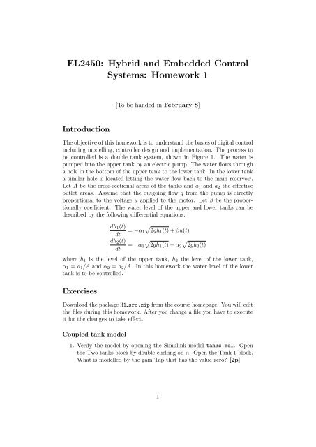
The objective of this homework is to understand the basics of digital control
including modelling, controller design and implementation. The process to
be controlled is a double tank system, shown in Figure 1. The water is
pumped into the upper tank by an electric pump. The water flows through
a hole in the bottom of the upper tank to the lower tank. In the lower tank
a similar hole is located letting the water flow back to the main reservoir.
Let A be the cross-sectional areas of the tanks and a 1 and a 2 the effective
outlet areas. Assume that the outgoing flow q from the pump is directly
proportional to the voltage u applied to the motor. Let β be the proportionally
coefficient. The water level of the upper and lower tanks can be
described by the following differential equations:
dh 1 (t) √
= −α 1 2gh1 (t) + βu(t)
dt
dh 2 (t) √ √
= α 1 2gh1 (t) − α 2 2gh2 (t)
dt
where h 1 is the level of the upper tank, h 2 the level of the lower tank,
α 1 = a 1 /A and α 2 = a 2 /A. In this homework the water level of the lower
tank is to be controlled.
Exercises
Download the package H1 src.zip from the course homepage. You will edit
the files during this homework. After you change a file you have to execute
it for the changes to take effect.
Coupled tank model
1. Verify the model by opening the Simulink model tanks.mdl. Open
the Two tanks block by double-clicking on it. Open the Tank 1 block.
What is modelled by the gain Tap that has the value zero? [2p]
1

Page 2 of 6 Homework Assigment 1 EL2450
Continuous control design
Figure 1: Coupled tanks with pump.
The scaled and linearized system is described by the transfer function
∆X 1 (s) =
k
1 + τs ∆U(s)
γ
∆X 2 (s) =
1 + γτs ∆X 1(s)
G(s) = ∆X 2 (s)
2. Edit the file pid_design.m and fill in the transfer functions for the
upper and lower tank. [1p]
We should now try to control the system. The design method that we
will use is pole-placement. We have the following step response requirements
on the closed loop system:
• rise time less than 6s
• overshoot less than 35%
• settling-time less than 30s
The PID-controller to be used is given by
[
F (s) = K 1 + 1
T I s + T ]
DNs
s + N
The closed loop system will have 4 poles. The poles will be placed using the
closed-loop characteristic equation
(s + χ) 2 (s 2 + 2ζω 0 s + ω 2 0) = 0
2

Page 3 of 6 Homework Assigment 1 EL2450
Input signal
Continous controller
r
F.num{1}(s)
F.den{1}(s)
u
h1
h2
Tank1 level
Referece signal
Two tanks
Tank2 level
Figure 2: Simulink model of closed loop system.
The calculation of the PID parameters is implemented in the function polePlacePID.m.
Open the file and make sure you understand how to use it.
3. Open the Simulink model by typing tanks. Also open the Simulink
model controller. Move the continuous controller to the tanks model
and connect them as shown in the Figure 2. Check the reference signal
block and describe what the reference signal will look like. [2p]
4. Edit the file pid_design.m. Use the function
[K_pid,Ti,Td,N]=polePlacePID(chi,omega0,zeta,Tau,Gamma,K)
to derive the PID parameters. Also fill in the transfer function for the
controller F . [2p]
χ ζ ω 0 T r M T settling
0.5 0.7 0.1
0.5 0.7 0.2
0.5 0.8 0.2
5. Simulate the system for the different values of the parameters as specified
in the table above. The first 100s of the simulation the system is
initializing, this part can be neglected when evaluating the control performance.
Which one of the parameter settings gives the best control
performance? [2p]
6. What is the cross over frequency of the open loop system? [1p]
Digital control design
The controller you just designed will be implemented digitally. This system
can be described as in the Figure 3. In this part of the homework, the A/D
and D/A converters can be neglected. This will be covered in the last part
of the homework. In Simulink, the sampling block is included at the input
3

Page 4 of 6 Homework Assigment 1 EL2450
Figure 3: Model of digital control system.
connector of all discrete blocks. Hence no explicit sampler is needed when
simulating the system with a discrete controller.
7. When implementing the controller digitally, what sampling time should
be used to keep the control performance? (Hint: Use the cross over
frequency of the open loop system). Enter the value in pid_design.m.
[2p]
8. Open the Simulink model. Disconnect the process from the rest of
the system to simulate it in open loop. Sample the system by connecting
a zero order hold block on the input and the output connector
of the process (remember to change its sample time). Use the calculated
sample time for the blocks. Plot the output from the sampled
open loop system when the input is a step. What are the differences
compared to the continues case? [5p]
9. Now simulate the system in closed loop again. Discretize the continuous
controller into state space form and remove the zero-order hold
block on the output connector of the process. Compare the simulation
result with the previous case when the continuous controller was used.
Are there any differences in control performance? [5p]
10. How long is the sampling interval possible without affecting control
performance? Compare with the calculated sampling time in Question
7 and comment on the possible differences. [3p]
Discrete control design
Now suppose that the sampling time is T s = 4.
11. Edit the file pid_design.m. Change the parameter T s to 4 and simulate
the system with the discretized controller. How is the control
performance affected? [1p]
We will now try a different approach. We will derive a sampled model of
the process for which we design a controller. The sampled model should be
on the form:
G d (z) = a 1z + a 2
z 2 + b 1 z + b2
4

Page 5 of 6 Homework Assigment 1 EL2450
The closed loop system should have the same performance as the continuoustime
closed loop, i.e., the systems should have the same poles. The discretetime
system poles are located at z i = e Tsp i
, where p i are the poles of the
continuous-time system. The controller to be designed is on the form:
F d (z) = c oz 2 + c 1 z + c 2
(z − 1)(z + r)
12. Sample the system G, with the sampling time T s = 4, using the
Matlab function c2d, with the zero-order hold method. Edit the file
pid_design.m and save the sampled system in the parameter Gd.
What are the coefficients a i and b i ? [3p]
13. Where should the poles of a discrete time system be located for it to
be stable? [1p]
14. Convert the poles for the continuous closed loop system to discretetime
poles. What are the corresponding poles for the discrete-time
closed loop system? Also calculate the corresponding pole polynomial
z 4 + d 0 z 3 + d 1 z 2 + d 2 z + d 3 . (Hint: Use the Matlab functions poly and
minreal.) [3p]
15. Now determine the controller parameters so that the closed loop system
gets the desired poles. Calculate the pole polynomial of the closed
loop system (1+F d G d ) −1 F d G d , set it equal to the desired discrete pole
polynomial and identify the coefficients. Show that this leads to the
following linear equations: [3p]
⎡
⎢
⎣
⎤
1 a 1 0 0
b 1 − 1 a 2 a 1 0
⎥
b 2 − b 1 0 a 2 a 1
⎦
−b 2 0 0 a 2
⎡ ⎤ ⎡
r
⎢ c 0
⎥
⎣ c 1
⎦ = ⎢
⎣
c 2
d 0 − b 1 + 1
d 1 − b 2 + b 1
d 2 + b 2
d 3
16. Solve the above equations and save the discrete controller in the variable
F d . Verify that the poles of the discrete-time closed loop system
are located where they should be. [2p]
17. Open the Simulink model and change to the discrete designed controller.
Simulate the system again and compare the coutcome with
previous cases. Conclusions? [2p]
Quantization
We will next investigate the effect of quantization. In a digital control system
quantization appears in three different parts. When the signal is converted
from analog to digital (A/D) the signal is quantized. The quantization level
depends on the number of bits of the converter. In the control algorithm
the output signal is computed. Here the size of the memory, used to store
the signal value, contributes to the quantization. The less memory used the
greater quantization. The conversion of the signal back to analog (D/A)
gives the same effect.
⎤
⎥
⎦ .
5

Page 6 of 6 Homework Assigment 1 EL2450
Figure 4: Quantizer with saturation.
18. Suppose you want to construct a A/D converter. The signal to be
converted vary between 0 and 100. What will the quantization level
be if the the number of bits used is 10? [3p]
19. In Simulink, the quantization block does not have any upper or lower
limits. Try to construct a quantization block by connecting a quantizer
with a saturation as shown in Figure 4. [2p]
20. Open the Simulink model with the discrete designed controller. Add
your own quantization block before and after the controller, both with
the same quantization level. This corresponds to a A/D and a D/A
converter. Set the saturation for both blocks to -100 for the lower and
100 for the upper limit. Simulate the system for different values of the
quantization level. For which quantization level will the control performance
start to be degraded? How many bits does this correspond
to? [5p]
6