ADVANCED USERS DMACRYS & NEIGHCRYS manual Manual ...
ADVANCED USERS DMACRYS & NEIGHCRYS manual Manual ...
ADVANCED USERS DMACRYS & NEIGHCRYS manual Manual ...

Create successful ePaper yourself
Turn your PDF publications into a flip-book with our unique Google optimized e-Paper software.
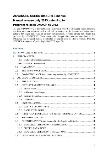
<strong>ADVANCED</strong> <strong>USERS</strong> <strong>DMACRYS</strong> <strong>manual</strong><br />
<strong>Manual</strong> release July 2013, referring to<br />
Program release <strong>DMACRYS</strong> 2.0.8<br />
The use of <strong>DMACRYS</strong> to calculate second derivative properties (including elastic constants<br />
and k=0 phonons), minimise with fixed cell parameters, apply pressure and adjust some<br />
defaults for larger molecules or difficult optimisations, requires editing the .dmain file<br />
produced by <strong>NEIGHCRYS</strong>. These commonly changed directives are described in 2.3.<br />
Otherwise this technical <strong>manual</strong> is intended for expert users to allow deviations from the<br />
<strong>NEIGHCRYS</strong> system of producing <strong>DMACRYS</strong> input files.<br />
Contents<br />
NOTATION (Used for data input) ............................................................................................ ii<br />
1 INTRODUCTION ............................................................................................................. 1<br />
1.1.1 Outline of what the program does .......................................................................... 1<br />
2 PRELIMINARY COMMENTS......................................................................................... 1<br />
2.1 DATA INPUT ............................................................................................................ 1<br />
2.2 THE INPUT PROCESSOR ....................................................................................... 2<br />
2.3 COMMON CHANGES to *.dmain as produced by <strong>NEIGHCRYS</strong> .......................... 2<br />
3 JOB STEPS IN <strong>DMACRYS</strong> .............................................................................................. 3<br />
3.1 TITLE SECTION....................................................................................................... 3<br />
3.2 DEFAULT PARAMETER CHANGES .................................................................... 4<br />
3.2.1 Printed output ......................................................................................................... 4<br />
3.2.2 Additional Input/Output ......................................................................................... 6<br />
3.2.3 Program Control..................................................................................................... 7<br />
3.2.4 CUTOFFS .............................................................................................................. 8<br />
3.3 UNIT CELL SETUP .................................................................................................. 9<br />
3.3.1 LATTICE VECTOR INPUT ................................................................................. 9<br />
3.3.2 BASIS ATOM INPUT ......................................................................................... 10<br />
3.4 INPUT POLARISABILITIES FOR INDUCTION CALCULATION.................... 13<br />
3.5 SPLINED POTENTIALS ........................................................................................ 13<br />
3.6 POTENTIAL INPUT (other than multipoles & polarizabilities) ............................ 14<br />
3.6.1 REPULSION-DISPERSION POTENTIAL INPUT ........................................... 14<br />
3.6.2 SPECIES DATA INPUT ..................................................................................... 15<br />
3.6.3 REPULSION-DISPERSION INTERACTIONS ................................................. 16<br />
3.7 INTRAMOLECULAR GEOMETRY SETUP ........................................................ 20<br />
i
3.8 DAMPING PARAMETER INPUT ......................................................................... 25<br />
3.9 PERFECT LATTICE CALCULATION ................................................................. 25<br />
3.9.1 Perfect Lattice Relaxation Control Parameters .................................................... 25<br />
3.9.2 Successful minimisation ...................................................................................... 34<br />
3.9.3 Output from additional optional directives .......................................................... 41<br />
3.10 PROPERTIES CALCULATIONS .......................................................................... 42<br />
3.10.1 Properties Calculations Control Parameters .................................................... 43<br />
3.10.2 Elastic Constants .............................................................................................. 44<br />
3.10.3 Phonon frequencies .......................................................................................... 45<br />
3.11 PRINT ANY ERROR MESSAGES ........................................................................ 46<br />
Appendix A. Full list of all directives written into the code ............................................. 47<br />
Appendix B. Options for printed output ............................................................................ 49<br />
Appendix C. Possible potentials ........................................................................................ 50<br />
Appendix D. Authors recommended potentials ................................................................ 58<br />
Appendix E. Possible control parameters for perfect lattice relaxation ................................ 61<br />
Appendix F. Lattice Vector and Basis input ......................................................................... 62<br />
Appendix G. Minimization Methods ................................................................................. 64<br />
Appendix H. Symmetry ..................................................................................................... 64<br />
NOTATION (Used for data input)<br />
Throughout the <strong>manual</strong> the following notation is used.<br />
_F The user must supply a floating point number in F format (Note that E format is<br />
not permitted).<br />
I The user must supply an integer.<br />
A The user must supply a character constant. Only the first four characters will be<br />
interpreted if it is a directive.<br />
F,I In some parts of the input dataset, the user has a choice of a real number or an<br />
integer.<br />
Optional parameters are enclosed in angle brackets.<br />
Italic script will be used for items in the printed output that depend on the input<br />
dataset.<br />
ii
1 INTRODUCTION<br />
This document describes the data input to the <strong>DMACRYS</strong> computer program. Normally the user will use the<br />
pre-processor <strong>NEIGHCRYS</strong> to write an input file template (file.dmain) and generate the symmetry file<br />
(fort.20). This <strong>manual</strong> provides details on the keywords for understanding the <strong>NEIGHCRYS</strong> generated<br />
<strong>DMACRYS</strong> input file (file.dmain), and making adaptations if there are problems with specific systems<br />
during the minimisations, including defining the error messages. It also shows additional options available in<br />
<strong>DMACRYS</strong>, including other potential forms, unusual crystal structures, additional printouts etc.<br />
1.1.1 Outline of what the program does<br />
It is possible to write an input file for <strong>DMACRYS</strong> without using <strong>NEIGHCRYS</strong>. This section outlines what<br />
needs to be input, greater detail follows in subsequent sections. (NB it is not possible to produce the<br />
additional file needed to use symmetry, described in Appendix H. so the keyword SYMM must be omitted).<br />
Data describing the unit cell is first read in together with the multipole expansion of the charges on each<br />
atom. All data must be supplied in orthonormal coordinates rather than conventional crystallographic<br />
coordinates. Next, atom-atom potentials are read in which model the crystal structure. Details of the<br />
molecular bonding are also supplied. The perfect lattice is then modelled using this potential. The variables<br />
are the centre of mass translations and three independent rotations of each rigid molecule, together with the<br />
unit cell constants. The most expensive part of the calculation in terms of computer time is usually the<br />
calculation of the gradients of the energy. These are calculated at every iteration of the energy minimisation.<br />
The minimisation uses a Hessian update algorithm, hence the second derivative matrix need only be<br />
calculated and inverted once. The second derivative matrix can be calculated either analytically (although<br />
not all of the terms have been worked out analytically) or numerically by differences (although this is much<br />
more expensive). For energy minimisation analytical second derivatives are preferred since the Hessian<br />
update algorithm gives a good approximation when the minimisation is complete. For properties<br />
calculations no minimisation is done and numerical second derivatives must be used. See NOPR directive<br />
below (Section 3.9.1) The matrix inversion step may be expensive for large unit cells. This is because the<br />
inversion increases as N 3 , whereas the gradient and matrix calculation increase as approximately N 2 .<br />
2 PRELIMINARY COMMENTS<br />
2.1 DATA INPUT<br />
<strong>DMACRYS</strong> uses a free format input processor. Each line of data is read in as characters, which make up a<br />
number of data fields separated by one or more spaces. By default 120 characters per line are read in,<br />
although this may be reduced using the IREC directive. The characters are then interpreted as literal<br />
(character string), constants, integers or real numbers. Literals are input as a string of characters of which at<br />
least one must be alphabetic, which cannot contain any embedded spaces in the constant. Only the first four<br />
characters will be interpreted by the program for a directive.<br />
Integer constants are input as a signed or unsigned integer, which again must not contain any embedded<br />
spaces.<br />
Real constants may only be input in the F format (10.00), and the E format (1.00E+1) is prohibited. A real<br />
constant will therefore consist of an optional sign, followed by a floating point number containing a decimal<br />
point. Again there should be no embedded spaces, and the decimal point should always be included.<br />
There is no end of record error message, so that attempting to read past the end of a line will not cause an<br />
error. If the program tries to read a literal constant and there are no more data fields in the record, four blank<br />
characters are input. Similarly for an integer the value 0 is input and for a real number the value 0.0.<br />
Error Messages<br />
Error - Invalid format for I variable<br />
The input processor encountered an invalid character in an integer data field.<br />
Error - Invalid format for F variable<br />
The input processor encountered an invalid character in a real data field.<br />
1
These are both non-fatal errors, the program may carry on in order trying to find further errors.<br />
End of file unit number 5 Program terminating<br />
This is a fatal error - the input dataset is too short.<br />
2.2 THE INPUT PROCESSOR<br />
<strong>NEIGHCRYS</strong> can be used to generate an input file for <strong>DMACRYS</strong> (file.dmain and associated fort.20<br />
symmetry file).<br />
The <strong>DMACRYS</strong> input dataset consists of a number of steps each containing one or more directives, which<br />
together form the main menu of the program. Each directive consists of a four-character keyword. Each of<br />
these directives may have data read in from the same record, or may instruct the program to read in further<br />
records before the next directive. These further records may consist of data, or they may be sub-directives<br />
instructing the program to choose one of several paths from a separate menu. For example, the potential<br />
input step has one directive, POTE, which instructs the program to read in potential information from<br />
subsequent records. The potential information is read in using a separate menu and records containing the<br />
data. The potential input menu contains a directive ENDS which instructs the program to return to the main<br />
menu. Care is needed in ordering the directives not to put a directive in the wrong place, for example a<br />
directive from the main menu when a sub-directive from the potential input menu is expected. Any errors<br />
detected in the input processor may not necessarily cause the program to stop immediately, to allow<br />
inexperienced users to find several errors in one run. A blank record is ignored if it is encountered when a<br />
directive from the main menu was expected, but not elsewhere. The steps in a <strong>DMACRYS</strong> job are outlined<br />
in Table 3.1 in the order in which they should be run, together with the directives from the main menu used<br />
in each step. A number of the directives are redundant but are kept for compatibility or future developments.<br />
The main menu directives MOLE and STAR PLUT both have large sub-menus of directives.<br />
2.3 COMMON CHANGES to *.dmain as produced by <strong>NEIGHCRYS</strong><br />
There are certain directives and control parameters that are more frequently changed from the defaults that<br />
<strong>NEIGHCRYS</strong> writes to file.dmain. These are listed in Table 2.1 with a brief description and link to the<br />
relevant section of the <strong>manual</strong>.<br />
Table 2.1 Commonly change directives from the defaults written out by <strong>NEIGHCRYS</strong><br />
DIRECTIVE COMMENT SECTION<br />
To optimise with fixed cell parameters<br />
CONV /CONP<br />
CONV replaces CONP to<br />
minimize with constant lattice<br />
3.9.1 CONV<br />
3.9.1 CONP<br />
vectors, instead of under constant<br />
(default zero) pressure<br />
To apply isotropic pressure<br />
PRES<br />
Insert to run <strong>DMACRYS</strong> for 3.9.1 PRES<br />
crystals under pressure<br />
To calculate second derivatives properties (after rerunning <strong>NEIGHCRYS</strong> on a successfully converged<br />
<strong>DMACRYS</strong> minimisation structure (fort.16)<br />
STAR PROP/PLUT<br />
NOPR<br />
Change <strong>NEIGHCRYS</strong> default of<br />
STAR PLUT to STAR PROP,<br />
and remove the NOPR line to stop<br />
the approximation of the second<br />
derivatives<br />
To change the lattice summation parameters<br />
CUTO<br />
The operand CUTPOT defines the<br />
repulsion-dispersion potential<br />
cutoff<br />
RDMA<br />
The operand RDMA defines the<br />
cutoff for the higher multipoles. It<br />
3.10 PROPERTIES<br />
CALCULATIONS<br />
Contrast<br />
3.9 PERFECT LATTICE<br />
CALCULATION<br />
3.9.1 NOPR<br />
3.2.4 CUTO<br />
3.2.4 RDMA<br />
2
SPLI<br />
ACCM<br />
is usually set to equal CUTPOT<br />
SMIN and SMAX are used to<br />
smooth the cutoffs of the<br />
multipole and repulsiondispersion<br />
interactions. It can be<br />
removed for an abrupt cutoff.<br />
To change Ewald summation<br />
3.6.3 SPLI<br />
3 JOB STEPS IN <strong>DMACRYS</strong><br />
Table 3.1: JOB STEPS IN A <strong>DMACRYS</strong> JOB.<br />
JOB STEP DIRECTIVES COMMENTS<br />
TITLE TITL, ENDS Optional<br />
DEFAULT PARAMETER<br />
CHANGES<br />
DUMP, PRIN, IREC, ACCU,<br />
ACCM, SCAL, SYMM, FDAT,<br />
CHGC, CLUS, ZVAL, EXTN<br />
Optional, order of steps may be<br />
varied<br />
CUTOFFS CUTO, RDMA Mandatory<br />
UNIT CELL SETUP including LATT<br />
atomic multipoles<br />
BASI<br />
Mandatory<br />
Order of directives must not be<br />
ENDS<br />
varied<br />
ATOMIC POLARIZABILITIES POLZ<br />
Optional, requires DIND<br />
ENDS<br />
SPLINE PARAMETERS SPLI Optional, but set by default in<br />
<strong>NEIGHCRYS</strong><br />
Other POTENTIAL INPUT POTE<br />
Mandatory<br />
ENDS<br />
MOLECULE INPUT<br />
MOLE<br />
Mandatory<br />
ENDS<br />
DAMPING PARAMETERS DDMP<br />
Optional<br />
DIND<br />
PERFECT LATTICE<br />
CALCULATION<br />
STAR PLUT<br />
Either STAR PLUT or STAR<br />
PROP are needed<br />
PROPERTIES<br />
STAR PROP<br />
CALCULATION<br />
STOP STOP Mandatory<br />
The full list of directives, including those that are seldom used or redundant, is given in Appendix A.<br />
The order of the job steps should not be varied, although variation from this order is permitted in certain<br />
cases. Firstly, some of the directives to change default parameters may be more conveniently placed later in<br />
the dataset. Where this is so it will be discussed in the section on the individual directives, and the default<br />
directives should otherwise always be placed where indicated. Secondly, the title step may appear more than<br />
once, anywhere in the sequence given above.<br />
Error Messages<br />
ERROR - Unidentified directive found in input data. The input line is as follows.<br />
This error does not cause the program to stop immediately. Further errors will be sought before the program<br />
stops. Check that the directive has been spelt correctly. Also this error message can arise if the input dataset<br />
is in the wrong order, and the input processor attempts to process either data or a directive from one of the<br />
sub-menus as a directive from the main menu.<br />
3.1 TITLE SECTION<br />
The title step has only one directive, TITL.<br />
3
Operands<br />
None<br />
TITL<br />
This directive instructs the program to read in and print a heading on the line printer output. Subsequent<br />
records will be read in and printed out exactly as input. The title is terminated with a record with the single<br />
word ENDS, which returns control to the main menu of the program. TITL directives may appear anywhere<br />
where a main menu directive can appear, but cannot be embedded in data.<br />
Example input<br />
TITL<br />
starting.res.dmain A1776_CrystalOptimizer<br />
ENDS<br />
3.2 DEFAULT PARAMETER CHANGES<br />
All of these directives are optional. They may be subdivided into two classes.<br />
Printed output<br />
DUMP, PRIN<br />
Program control IREC, ACCU, ACCM, CHGC, SCAL, CLUS, SYMM, FDAT, ZVAL<br />
3.2.1 Printed output<br />
Operand type<br />
Operand name<br />
I<br />
IDUMP<br />
DUMP<br />
This is used in conjunction with the PRIN directive discussed below. IDUMP may have values 1 or 2.<br />
IDUMP = 1 produces output which may be useful if an error is suspected in the input dataset. IDUMP = 2<br />
produces output useful for diagnostic purposes only.<br />
PRIN<br />
Operand types A I [ A I ... ...]<br />
Operand names APRINT MPRINT<br />
The APRINT name defines certain sections of the program for which additional printed output is required.<br />
The integers MPRINT define exactly what is printed. There are currently 6 print options for <strong>DMACRYS</strong>.<br />
Each of these will now be described in detail.<br />
PLUT<br />
MPRINT is a 5 digit integer, with each digit controlling a different section of the perfect<br />
lattice calculation. Numbering the digits from the right (units digit) to left the digits have the<br />
following values and meanings.<br />
Digit 1<br />
Digit 2<br />
0<br />
1<br />
2<br />
No output<br />
List the contributions to the lattice energy and<br />
the atom forces before the first iteration and<br />
after the last iteration.<br />
List the contributions to the lattice energy after<br />
each iteration.<br />
As for digit 1 but listing the elastic constant tensors.<br />
4
LATT<br />
BASI<br />
Digit 3<br />
Digit 4<br />
Digit 5<br />
0<br />
0<br />
1<br />
2<br />
3<br />
No output<br />
No output<br />
List the force constant matrix and gradient<br />
vector before the first cycle and after the last<br />
cycle.<br />
List the force constant matrix and gradient<br />
vector on every cycle of the perfect lattice<br />
iteration.<br />
List the gradient vector only before the first<br />
cycle and after the last cycle<br />
4<br />
List the gradient vector only on every cycle<br />
The force constants are scaled in internal program units. To convert to<br />
(eV Å)-2 they must be multiplied by 14.3997584/RLSCAL3, where<br />
RLSCAL is the lattice constant. The gradients must be scaled by<br />
14.3997584/RLSCAL2.<br />
0<br />
No output<br />
1<br />
Currently not used, formerly used to print the<br />
Madelung and repulsion-dispersion energies of<br />
each particle. (Use CCLS instead)<br />
Default 00011 - <strong>NEIGHCRYS</strong> default is 00012<br />
0<br />
> 0<br />
Default 0<br />
0<br />
> 0<br />
No output<br />
The reciprocal lattice<br />
vectors are printed in<br />
the output.<br />
Print:<br />
In addition, print:<br />
Basis atoms as input<br />
Origin of the basis<br />
The basis atoms after shift of origin<br />
The basis atoms after sorting into internal<br />
5
MINI<br />
MOLE<br />
GEOM<br />
< 0<br />
Default 0<br />
Suppress printing of<br />
the basis atoms<br />
program order<br />
0<br />
No output<br />
1<br />
Print information about progress of the minimisation.<br />
2<br />
As 1 plus lattice energies<br />
3<br />
As 2 plus individual contributions to the lattice energy<br />
4<br />
As 3 plus first part of the hessian<br />
Default 0 – <strong>NEIGHCRYS</strong> default is 2<br />
This APRINT option is used in <strong>DMACRYS</strong> to control output from the MOLE directive.<br />
0<br />
Do not print molecular bonding information.<br />
1<br />
Print molecular bonding information<br />
Default 1<br />
0<br />
1<br />
Default 1<br />
No output<br />
Print molecular local axis information<br />
The full list of printing options, including those that are redundant, is given in Appendix B.<br />
Example input<br />
PRIN BASI 0 PLUT 12 MOLE 1 BOND 2 TORS 2 MINI 2 GEOM 1<br />
Printed output<br />
The printing options are as follows.<br />
PLUT LATT BASI MINI MOLE GEOM<br />
12 0 0 2 1 1<br />
3.2.2 Additional Input/Output<br />
Table 3.2 gives a list of the additional FORTRAN unit numbers used by <strong>DMACRYS</strong>. Output is produced by<br />
default to fort.8, fort.12, fort.13, fort.15, and fort.16.<br />
Table 3.2: ADDITIONAL FORTRAN UNIT NUMBERS USED BY PROGRAMS<br />
DIRECTIVE UNIT NATURE OF I/O USE<br />
STAR PLUT 8 FORMATTED WRITE Provides an updated set of lattice and basis<br />
vectors from the perfect lattice relaxation<br />
Default 12 FORMATTED WRITE Summary file written to fort.12<br />
Default 13 FORMATTED WRITE Final cell written to fort.13<br />
Default 15 FORMATTED WRITE Final output in FDAT format<br />
Default 16 FORMATTED WRITE Final output in SHELX format<br />
6
CCLS 17 FORMATTED WRITE Output close contact list to fort.17<br />
SYMM 20 FORMATTED READ Read the symmetry information file fort.20<br />
written by <strong>NEIGHCRYS</strong><br />
R2ND 30 FORMATTED<br />
READ/WRITE<br />
Temporary file used for restart runs.<br />
3.2.3 Program Control<br />
Operand type<br />
Operand name<br />
I<br />
IRECL<br />
IREC<br />
The input processor reads 120 characters per card image by default. IRECL should be less than 120, and<br />
gives the number of characters read in per record.<br />
ACCU<br />
Operand type<br />
F<br />
Operand name<br />
ACCLAT<br />
ACCLAT is the limit below which numbers are taken as being equal. The default set in the program is 1.0E-<br />
06. ACCLAT is also used at various other points in the program for testing small quantities.<br />
ACCM<br />
Operand type<br />
F <br />
Operand name<br />
ACCMAD RLWGT<br />
This directive changes the accuracy to which the Ewald sum is carried out. The default for ACCMAD is 1<br />
part in 10 6 (Default value of ACCMAD = 1000000.0). RLWGT changes the weighting towards carrying out<br />
the Ewald sum in reciprocal space as opposed to direct space and its default value is 1.0. RLWGT can be<br />
used to fine tune the Ewald sum, but altering its value from 1.0 should not make any significant difference to<br />
the calculation. Setting a larger value of RLWGT will carry out more of the calculation in reciprocal space,<br />
but the calculation may take longer. Values of RLWGT between 0.25 and 4.0 could be used. Setting a larger<br />
value of ACCMAD may change the perfect lattice properties slightly. It should also be noted that a larger<br />
value of ACCMAD will set a larger lattice sum cutoff and the calculation will take longer.<br />
SCAL<br />
Operand type<br />
F<br />
Operand name<br />
SCALQQ<br />
The charge and multipole interactions will be scaled by the factor SCALQQ. This is set by default in<br />
<strong>NEIGHCRYS</strong> to 1.0<br />
SYMM<br />
Operands<br />
None<br />
Instructs <strong>DMACRYS</strong> to read in the symmetry input file fort.20 that was written by <strong>NEIGHCRYS</strong>. This is<br />
set by default in <strong>NEIGHCRYS</strong>. If SYMM is removed, the structure will relax with no symmetry, however it<br />
is preferable to lower the symmetry to P1 in <strong>NEIGHCRYS</strong> rather than use this option.<br />
Operands<br />
None<br />
FDAT<br />
Instructs <strong>DMACRYS</strong> to read in the symmetry input file fort.20 that was written by <strong>NEIGHCRYS</strong>, but not to<br />
switch on symmetry for this run. This option is useful for producing a final relaxed structure dataset from a<br />
run with no symmetry.<br />
7
Operands<br />
None<br />
CHGC<br />
The programs checks that the unit cell is neutral and will stop if it is not. Including the directive CHGC<br />
forces the program to continue with a non-neutral cell. DMAs generated by SCF programs often have a<br />
small residual charge, so this directive should be included and is set by <strong>NEIGHCRYS</strong>.<br />
CLUS<br />
Operands<br />
None<br />
This directive tells <strong>DMACRYS</strong> to switch off the Ewald sum and carry out charge-charge and charge-dipole<br />
interactions by direct summation. This can be used to work out the energy of a cluster by using a cell with<br />
artificially large lattice vectors.<br />
ZVAL<br />
Operand type<br />
I<br />
Operand name<br />
ZVAL<br />
ZVAL is the user-defined number of formula units per cell, used to calculate energies in kilojoules per mole.<br />
If ZVAL is not supplied, <strong>DMACRYS</strong> will try to read it from the fort.20 file.<br />
EXTN<br />
Operand type<br />
F<br />
Operand name<br />
EXTH<br />
This directive is used in conjunction with the Williams potential. If <strong>NEIGHCRYS</strong> uses the Williams<br />
potential, EXTN 0.1 will be written<br />
The Williams potential uses artificially shortened hydrogen bond lengths by moving the positions of the<br />
hydrogen atoms. This is to take some account of the effect of thermal motion in the crystal. If <strong>NEIGHCRYS</strong><br />
is used to set up the dmain file, the hydrogen atoms can be foreshortened by using the appropriate option in<br />
the <strong>NEIGHCRYS</strong> input. <strong>NEIGHCRYS</strong> always foreshortens the H atom positions by 0.1 Angstroms. The<br />
directive EXTN instructs <strong>DMACRYS</strong> to extend the hydrogen bond lengths by an amount EXTH Angstroms.<br />
This will be done before the final fdat and res files are written to units 15 and 16 respectively so that the job<br />
may be restarted to carry out a symmetry reduction or properties calculation without cumulative reductions<br />
in the H bond length taking place. EXTH should be set to 0.1 for datasets written by <strong>NEIGHCRYS</strong> but may<br />
need to be set to other values if the foreshortening is not 0.1.<br />
3.2.4 CUTOFFS<br />
CUTO<br />
Operand types F F <br />
Operand names RLSCAL CUTPOT ACCTH CUTTH<br />
CUTOFFS<br />
The repulsion-dispersion interactions which are calculated in <strong>DMACRYS</strong> are controlled by two cutoffs,<br />
CUTPOT and RDMA.<br />
RLSCAL gives the lattice constant c in Å. (See LATT and BASI directives and the examples following).<br />
Certain quantities are input in units of RLSCAL, referred to as lattice units.<br />
CUTPOT gives the repulsion-dispersion potential cutoff in lattice units. CUTPOT should not be equal to an<br />
interatomic distance in the crystal. This is because the test in the perfect lattice calculation may find one<br />
bond but leave out a symmetry related bond, giving perfect lattice tensor properties of the wrong symmetry.<br />
Usually it is safe just to ensure that CUTPOT does not equal an integral number of lattice vectors. (i.e. that<br />
CUTPOT is not an integer). <strong>NEIGHCRYS</strong> will set a default value of 15 Å.<br />
8
The ACCTH operand is retained for future use, but is not used at present. Its value is ignored if the<br />
calculation does not use three-body forces. It gives the maximum permitted deviation of a bond angle from<br />
the value input on the BOHA sub-directive of the POTE directive. This maximum deviation is applied in the<br />
perfect lattice step to check that no spurious three-body interactions have been generated by the THBO<br />
directive.<br />
The CUTTH operand is retained for future use, but is not used at present.<br />
The cutoffs are used with the range parameters on the input potentials. The potentials may be input over a<br />
number of ranges, although usually only one range is used. The parameter defining the ranges is intended<br />
primarily as a separation of two ranges and not as a cutoff of the potential. Therefore the maximum range of<br />
the potential is always overridden by the value of CUTPOT. Thus if the maximum range is greater than<br />
CUTPOT, then interactions will only be calculated out to CUTPOT. If the maximum range is input as a<br />
value less than CUTPOT, its value is redefined and set to a value larger than CUTPOT.<br />
Example input<br />
CUTO 6.999700 2.142949<br />
RDMA 2.142949<br />
Printed Output<br />
C-vector magnitude= RLSCAL Angstroms<br />
Cut off for repulsion-dispersion potentials = Cutpot*RLSCAL Angstroms<br />
Example output<br />
C-vector magnitude= 6.999700 Angstroms<br />
Cut off for repulsion-dispersion potentials = 15.000000 Angstroms<br />
RDMA<br />
Operand type<br />
F<br />
Operand name<br />
RANG<br />
This gives the cutoff in lattice units for the higher multipoles. <strong>NEIGHCRYS</strong> will set a default value of 15 Å.<br />
Higher multipoles are calculated for all atoms within two molecules whose centres of mass are within<br />
RDMA.<br />
Printed Output<br />
Cut off for higher multipole summation =<br />
Example output<br />
Cut off for higher multipole summation =<br />
3.3 UNIT CELL SETUP<br />
RANG*RLSCAL Angstroms<br />
15.00000012 Angstroms<br />
This section reads in the unit cell. These directives must be given in the order<br />
LATT, BASI<br />
3.3.1 LATTICE VECTOR INPUT<br />
LATT<br />
Operands<br />
None<br />
This directive is required. The LATT directive instructs the program to call the lattice vector input routine.<br />
The calculations are described in appendix E. They are performed by the pre-processor <strong>NEIGHCRYS</strong>.<br />
Example input<br />
LATT<br />
Printed output<br />
1.4092175378945 0.0000000000000 0.0000000000000<br />
0.0000000000000 1.4485049359258 0.0000000000000<br />
0.0000000000000 0.0000000000000 1.0000000000000<br />
9
The lattice vectors are always printed by default. They are printed in rows, with the x, y, z components of<br />
each lattice vector in each row. If PRIN LATT MPRINT with MPRINT=1 is used, the reciprocal lattice<br />
vectors are also printed, again in rows.<br />
START OF LATTICE VECTOR PROCESSING.<br />
THE LATTICE VECTORS ARE AS FOLLOWS.<br />
XLAT(1,1) XLAT(2,1) XLAT(3,1)<br />
XLAT(1,2) XLAT(2,2) XLAT(3,2)<br />
XLAT(1,3) XLAT(2,3) XLAT(3,3)<br />
Example output<br />
START OF LATTICE VECTOR PROCESSING.<br />
THE LATTICE VECTORS ARE AS FOLLOWS.<br />
1.409217537894501 0.000000000000000 0.000000000000000<br />
0.000000000000000 1.448504935925801 0.000000000000000<br />
0.000000000000000 0.000000000000000 1.000000000000001<br />
Error messages<br />
ERROR - lattice vectors not defined before crystal basis.<br />
This is a fatal error. The program decided that the lattice vectors are coplanar by working out the volume of<br />
the unit cell, which is equal to the determinant of the lattice vector matrix. This is tested to see if it is greater<br />
than ACCLAT (see ACCU directive).<br />
Error - Invalid format for F variable<br />
A fatal error, there is a format error in one of the lattice vector input records.<br />
3.3.2 BASIS ATOM INPUT<br />
Operands<br />
None<br />
BASI<br />
The BASI directive instructs the program to call the basis atom input routine. Usually the calculations<br />
described below will be carried out using the pre-processor <strong>NEIGHCRYS</strong>. This reads in further records,<br />
which have one of three possible formats<br />
Card format A15 3F < I ><br />
Long atom label Atom coordinates Optional molecule<br />
number<br />
Card format A 3F<br />
CENT<br />
Point group origin<br />
Card format<br />
A<br />
ENDS<br />
Only one CENT and ENDS record is permitted. The CENT record defines the basis origin. This record is<br />
not required for <strong>DMACRYS</strong>, it may be omitted, in which case the basis origin is taken as the point 0.0 0.0<br />
0.0. The ENDS record must be the last record, and instructs the subroutine to return to the main menu of<br />
directives.<br />
There may be any number of atom records up to a maximum of MAXBAS (this includes the CENT record if<br />
present). The long atom label consists of an A15 field made up as follows. The first two characters are the<br />
element type and make the element label. Where an element has only 1 letter has an underscore is used as<br />
the second character. The third and fourth characters denote the type of repulsion-dispersion potential, for<br />
example where the potential includes different terms for different types of hydrogen atom. The first four<br />
characters together make up the species label defining a unique element and potential type. The fifth<br />
character is _ or I, where I denotes the atom is part of an inverted molecule. The sixth to tenth characters<br />
number the atoms, where equivalent atoms in different molecules have the same number. Where the atom<br />
number is shorter than 5 digits long, the remaining characters are filled with the underscore symbol. The<br />
number starts from the left. The first 10 characters make up the short atom label. The long atom label<br />
comprises the short atom label and 5 further characters denoting the number of the atom in the entire unit<br />
cell.<br />
10
H_F1_1_____ would be the short atom label of a hydrogen atom with the F1 potential type, not in an<br />
inverted molecule, and the first hydrogen atom of this molecule.<br />
Similar comments apply about the precision as for the lattice vectors, namely the coordinates must be given<br />
to at least 7 significant figures unless the ACCU directive has been used. The optional molecule number is<br />
used to indicate to which molecule it belongs. A value of zero, or leaving out the parameter all together,<br />
implies that intramolecular potentials will not be applied to this atom, and is used for isolated ions. Isolated<br />
ions should be put at the end of the list; <strong>NEIGHCRYS</strong> will do this automatically.<br />
The distributed multipoles must be given for the atoms.<br />
Operand type A I<br />
Operand name LEVEL ORDER<br />
The record following the atom coordinates must begin with the keyword LEVEL or DUPL. Use LEVEL the<br />
first time an atom is encountered, use DUPL for duplications. LEVEL is followed by an integer indicating<br />
the pole order of the multipole on this atom, 0 for charge only up to 4 for hexadecapole. The atom’s charge<br />
is given in units of | e| (The charge on the electron). The multipoles are then given in atomic units. The<br />
format is<br />
Operand type<br />
F<br />
F F F<br />
F F F F F<br />
F F F F F F F<br />
F F F F F F F<br />
F F<br />
Operand name<br />
CHARGE<br />
The operands are one charge, three dipole, five quadrupole, seven octopole and nine hexadecapole moments<br />
in the usual order. This will usually be input from the dma file in <strong>NEIGHCRYS</strong>.<br />
It should be noted that adding or subtracting a lattice vector, or an intergal multiple of a lattice vector, to a<br />
basis vector will have no effect on the program. In other words, basis atoms need not all be in the same unit<br />
cell.<br />
The basis atoms will be sorted into an internal program order, but this will normally be done by<br />
<strong>NEIGHCRYS</strong>. The order into which they are sorted is determined by a number of rules.<br />
1. All atoms in molecules come before free ions.<br />
2. All atoms with the same element label are sorted together<br />
3. All atoms with the same short atom label are sorted together.<br />
The Ewald parameter is also calculated at this point, according to the formula<br />
1/ 6<br />
3<br />
<br />
NCOR<br />
<br />
<br />
2<br />
<br />
V <br />
where<br />
NCOR = Number of atoms in the unit cell<br />
V = Volume of the unit cell in (lattice units) 3 .<br />
This is used with the parameter ACCMAD (see ACCM directive) to define the cutoffs in direct and<br />
reciprocal space for the Ewald sums.<br />
Direct space cutoff = f / η<br />
Reciprocal space cutoff = f × η/π<br />
f =<br />
log ACCMAD<br />
11
Example input<br />
BASI<br />
C_F1_1____1____ 1.1101807730993 0.0115731054015 0.1185363100000 1<br />
LEVEL 4<br />
-0.083010<br />
0.000208 0.018691 0.030772<br />
-0.985535 0.000338 -0.000982 -0.038430 0.230443<br />
-0.001680 -0.163223 -0.177082 -0.000341 -0.002022 -2.077258 0.179549<br />
-0.862134 -0.001088 0.000299 -0.508677 1.765922 -0.003956 -0.000607<br />
0.964204 1.430481<br />
C_F1_1____9____ 0.4055720041520 0.7126793625614 0.8814636900000 2<br />
DUPL<br />
Printed output<br />
the x basis species are as follows.<br />
all quantities are in lattice units<br />
no. orthogonal coordinates label molecule<br />
x y z<br />
index x y z label molecule<br />
Origin of basis<br />
0.000000000000000 0.000000000000000 0.000000000000000<br />
Basis origin shifted<br />
Example output<br />
the 64 basis species are as follows.<br />
all quantities are in lattice units<br />
no. orthogonal coordinates label molecule<br />
x y z<br />
1 1.11018077 0.01157311 0.11853631 C_F1_1____1____ 1<br />
2 0.40557200 0.71267936 0.88146369 C_F1_1____9____ 2<br />
3 0.29903676 0.73582557 0.38146369 C_F1_1____10___ 3<br />
<br />
Origin of basis<br />
0.00000000 0.00000000 0.00000000<br />
Basis origin shifted<br />
The basis atoms and basis origin are printed as input by default. PRIN BASI -1 will suppress printing of the<br />
basis atoms. PRIN BASI 1 will print additionally the basis atoms after sorting and after the point group<br />
origin vector has been subtracted from them.<br />
Printed output<br />
Cut off value for direct lattice sum = CUTLAT lattice units<br />
Cut off value for reciprocal lattice sum = CUTRLT reciprocal lattice units<br />
Values of the constants used in these summations are:<br />
Eta parameter for division of sum between real and reciprocal lattice= HFCT0<br />
PI/(ETA^2 * Vol.Cell) = GFCT0<br />
Example output<br />
Cut off value for direct lattice sum = 1.330080 lattice units<br />
Cut off value for reciprocal lattice sum = 3.306277 reciprocal lattice units<br />
Values of the constants used in these summations are:<br />
Eta parameter for division of sum between real and reciprocal lattice= 2.794510<br />
PI/(ETA^2 * Vol.Cell) = 0.197079<br />
This message is printed by default.<br />
Error messages<br />
ERROR - lattice vectors not defined before crystal basis.<br />
A LATT directive has been omitted or placed out of order, it should occur before the BASI directive.<br />
ERROR - Maximum of maxbas basis atoms exceeded.<br />
This error does not cause the program to terminate immediately.<br />
ERROR - Basis atoms i and j are at equivalent lattice sites.<br />
12
Two basis atoms have been found at the same lattice site. They may be at the same lattice site translated by<br />
an integral number of lattice vectors, so the coordinates are not necessarily the same.<br />
3.4 INPUT POLARISABILITIES FOR INDUCTION CALCULATION<br />
Operands<br />
None<br />
POLZ<br />
The POLZ directive instructs the program to read in the atom polarisabilities. Usually these will be read in<br />
by <strong>NEIGHCRYS</strong>. This reads in further records, which have one of two possible formats<br />
Card format A15 3F < I ><br />
Long atom label Atom coordinates Optional molecule<br />
Card format<br />
A<br />
ENDS<br />
number<br />
The label and atom coordinates must be the same as one of the input basis atoms. The record following the<br />
atom coordinates must begin with the keyword LEVEL or DUPL. Use LEVEL the first time an atom is<br />
encountered, use DUPL for duplications. LEVEL is followed by the integer 2. The format is of the following<br />
records is<br />
Operand type<br />
F<br />
F F<br />
F F F<br />
The operands are the components of the atomic polarisability.<br />
3.5 SPLINED POTENTIALS<br />
An abrupt cutoff in the direct summation of energies can lead to discontinuities in the energy as atoms (or<br />
entire molecules for the higher multipole terms) move over the cutoff boundaries or in and out of the stored<br />
list of close contacts. Although the cutoffs (given by CUTO & RDMA in units of c) should be set such that<br />
these terms are very small, this produces noise in the numerical first derivatives which are used in<br />
applications such as Crystal Optimizer or when optimizing the structure including the induction energy.<br />
Continuity in the numerical derivatives can be assured by introducing the command,<br />
SPLI DSPL1 DSPL2<br />
for example,<br />
SPLI 2.0 4.0<br />
directly above the POTE command. This adds a spline curve that matches the energy and first derivative of<br />
each term in the potential from its value at the cutoff and reduces to zero value and first derivative over a<br />
distance DSPL1 (= 2.0) Å. The close contacts list is calculated to DSPL2 (4.0) Å beyond the cutoff to<br />
ensure that this does not change during the calculation.<br />
The inclusion of SPLI thus adds to the repulsion-dispersion contribution the spline energy for all atoms lying<br />
between CUTO and CUTO + DSPL1, which will be a stabilising energy as all such contributions start from<br />
an attractive dispersion energy.<br />
The addition of splines changes the way that the higher multipole energies are calculated. Without a splined<br />
function, all higher multipole interactions between whole molecules whose centres of mass are within the<br />
cutoff, RDMA, are included. The table of molecules with centres within RDMA is set up at the beginning of<br />
the run, and not changed during the run, to avoid discontinuities in the energies from molecules appearing in<br />
the summation. When SPLI set, all higher multipole interactions with intermolecular atom-atom distances<br />
within RDMA are evaluated, plus the spline energies over the atom-atom range RDMA + DSPL1. The<br />
molecule table, set at the beginning of the run, is calculated out to a distance RDMA + 0.5 (maximum<br />
intramolecular distance) + DSPL2. The holding of the additional molecules in this table means that any<br />
13
molecules moving so their centres of mass within RDMA are now included in the higher multipole<br />
calculation. This aspect is a significant improvement on the original method for long molecules and small<br />
RDMA values (e.g. <strong>NEIGHCRYS</strong> default 15 Å).<br />
The spline is also applied to the electrostatic contributions calculated by Ewald summation. Hence the direct<br />
summation is out to the automatically determined direct summation limit + DSPL2, and differs from the true<br />
value by the difference between the true and spline values over the additional DSPL2 range. The cutoff<br />
value for the reciprocal lattice sum and the value of ETA are automatically adjusted to match the actual<br />
direct summation limit including DSPL2. The default accuracy of the Ewald summations means that the<br />
change in the Ewald summed terms is much smaller than the other terms.<br />
Currently <strong>NEIGHCRYS</strong>2.0.8 automatically adds the SPLI command.<br />
Printed output<br />
Potentials will be cutoff with a spline terminating at<br />
with limit in expansion set to splmax Angstroms<br />
splmin Angstroms<br />
Cut off value for direct lattice sum = CUTLAT lattice units<br />
Cut off value for reciprocal lattice sum = CUTRLT reciprocal lattice units<br />
Values of the constants used in these summations are:<br />
Eta parameter for division of sum between real and reciprocal lattice= HFCT0<br />
PI/(ETA^2 * Vol.Cell) = GFCT0<br />
Example output<br />
Potentials will be cutoff with a spline terminating at 2.00Angstroms<br />
with limit in expansion set to 4.00 Angstroms<br />
Cut off value for direct lattice sum = 1.901533 lattice units<br />
Cut off value for reciprocal lattice sum = 2.312667 reciprocal lattice units<br />
Values of the constants used in these summations are:<br />
Eta parameter for division of sum between real and reciprocal lattice= 1.954697<br />
PI/(ETA^2 * Vol.Cell) = 0.402803<br />
This change in the Ewald summation parameters is written out after the original data without a spline.<br />
3.6 POTENTIAL INPUT (other than multipoles & polarizabilities)<br />
3.6.1 REPULSION-DISPERSION POTENTIAL INPUT<br />
Operands<br />
None<br />
POTE<br />
This directive instructs the program to call the repulsion-dispersion potential input routine. This routine is<br />
menu driven with a menu of sub-directives. The sub-directives fall into seven classes: species data, repulsion<br />
& dispersion interactions, [core-shell interactions, three-body interactions, torsion interactions, restart subdirectives]<br />
and subroutine termination. Those in [] are not relevant to this version of <strong>DMACRYS</strong> but are<br />
retained for future use. Table 3.3 gives the sub-directives in each class.<br />
Table 3.3: DIRECTIVES FOR THE POTENTIAL INPUT SUBROUTINE<br />
Directive class<br />
Species data<br />
Repulsion-dispersion interactions<br />
Three-body interactions<br />
Four-body interactions<br />
The full list of potentials available is given in Appendix C.<br />
Directives<br />
SPEC, ENDS<br />
BUCK, MODI, LENN, MORS, BUC4, SPLP,<br />
MORQ, SPRI, COUL, VDWA, HULB, BUC7,<br />
NONE, BSPL,DBUC<br />
BOHA, TRID, MOLD, QART, SIXT, BOHZ,<br />
THRH, RRHA<br />
TOHA<br />
14
The directive order for the initial call must be<br />
Directives<br />
SPEC<br />
Others<br />
ENDS<br />
Comments<br />
Followed by subdirectives (See below)<br />
May be given in any order<br />
The limits on the numbers of potentials etc. are determined by a number of PARAMETER statements in the<br />
FORTRAN. These limits may be reset simply by changing every occurrence of the PARAMETER statement<br />
to the new limit. The variable names and default limits are given in Table 3.4.<br />
Table 3.4: POTENTIAL PARAMETERS LIMITS<br />
Variable Default Value Meaning<br />
MAXPOT 1000 Maximum permitted number of potentials<br />
MAXRNG 10 Maximum number of ranges for each potential<br />
MAXTYP 1000 Maximum number of short atom labels permitted<br />
MAXTHB 50 Maximum number of types of three-body bond<br />
MAXTOR 50 Maximum number of types of torsions<br />
Printed output and error messages from this section of the program are given below. Printed output may be<br />
suppressed using the option PRIN POTE 0 in the default parameter changes.<br />
Printed output<br />
START OF REPULSION-DISPERSION POTENTIAL PROCESSING<br />
This is always output by the program.<br />
Error messages<br />
ERROR - Invalid directive given in above line<br />
The line above began with an invalid directive.<br />
ERROR - SPECIES MUST BE READ IN BEFORE POTENTIALS<br />
The program has read in a valid potential input directive, but the species have not yet been read in using<br />
SPEC.<br />
ERROR - ABOVE LINE CONTAINS A SPEC DIRECTIVE - ONLY ONE IS PERMITTED<br />
Only one SPEC directive is permitted.<br />
3.6.2 SPECIES DATA INPUT<br />
SPEC<br />
Operands<br />
None<br />
This should be the first directive after POTE. It instructs the program to read in the elements and atomic<br />
masses. The subsequent data cards have the formats<br />
Card format A F F<br />
Element label Not used Atomic mass<br />
Card format<br />
A<br />
ENDS<br />
The element label is described in the BASI directive (3.3.2). The atomic mass is given in atomic mass units.<br />
A maximum of MAXTYP element labels may be read in. Element labels may be given which are<br />
superfluous to this particular job. The element input terminates with a directive ENDS, which returns control<br />
to the POTE menu of directives.<br />
Example input<br />
POTE<br />
SPEC<br />
C_ 0.0 12.010700<br />
O_ 0.0 15.999400<br />
15
H_ 0.0 1.007940<br />
ENDS<br />
Error messages<br />
These should be self-explanatory.<br />
Warning - A element has been given with zero or negative mass<br />
Warning - no mass is given for element label A10 set to 1.0<br />
ERROR - THE ELEMENT TYPE Lab Type IS DUPLICATED<br />
ERROR - THE LIMIT OF Maxtyp ELEMENT IS EXCEEDED<br />
3.6.3 REPULSION-DISPERSION INTERACTIONS<br />
Repulsion-dispersion interactions need to be given between some or all of the possible species pairs. The<br />
repulsion-dispersion interaction is designed to be as flexible as possible, although for <strong>DMACRYS</strong> only a<br />
few options will normally be used. Different species pairs may have different repulsion-dispersion<br />
interaction types. The repulsion-dispersion interactions are given in one or more ranges for each species pair,<br />
up to a maximum of MAXRNG ranges. For each species pair, the ranges must be contiguous and there must<br />
be a range which starts at zero. Interactions which have a different analytic form in different ranges are<br />
permitted. In this case, overlapping ranges are not permitted. However it is permitted to split one of the<br />
interactions into two ranges so that a range is the sum of two potentials. The ranges, if more than one range<br />
is given, must be in ascending order. The maximum range is at present overridden by CUTPOT. (See section<br />
on cutoffs) A maximum of MAXPOT repulsion-dispersion interactions may be given.<br />
The general format of a repulsion-dispersion interaction is given below. There are three types of input<br />
records. Species records indicate the start of a new two body interaction and give the two species involved.<br />
Species records begin with the type of interaction involved, and include the two species labels, which are the<br />
first 4 characters of the atom label. An interaction may have more than one species record, for example<br />
where different potential forms are required for different ranges. Range records give the parameters for the<br />
interaction in a given range. Finally, an ENDS record terminates the input for all potential forms and ranges<br />
for a particular species pair. The format of a species record is<br />
Card format A4 A4 A4 < F,I ><br />
Potential type Species label A Species label B<br />
(see 3.3.2) (see 3.3.2)<br />
Card format F … < F > F<br />
Parameters Optional RMIN RMAX<br />
Additional<br />
Parameters for<br />
certain potential<br />
types only<br />
RMIN and RMAX define the minimum and maximum range for this potential. RMIN may be omitted; the<br />
program knows how many parameters there are on the record and can therefore determine whether an RMIN<br />
has been given. If RMIN is omitted, the program uses the following rules to decide which value it should<br />
have.<br />
If it is the first range record after a species record, the minimum range is assumed to be zero.<br />
If it is a subsequent range, the minimum range is taken as the maximum of the previous range.<br />
If a second species record is given, the ranges must either coincide with ranges given after the first species<br />
record or must be new ranges, contiguous with the existing ranges but extending beyond the previous<br />
maximum. Overlapping ranges are not permitted. The limits of the ranges are given in Å so that no<br />
conversion needs to be done when the data is transferred to a different substance. (cf. the CUTPOT<br />
parameter, which is in lattice units.)<br />
Example input<br />
BUCK C_F1 C_F1<br />
3832.147000 0.27777800 25.286950 0.00 70.00<br />
ENDS<br />
Printed output<br />
16
POTENTIAL BETWEEN SPECIES JSPECA AND JSPECB WITH JRANGF RANGES<br />
LIST OF GENERAL INTERACTIONS<br />
This indicates that the interaction is intermolecular.<br />
Error messages<br />
A number of error messages will be given here as they do not depend on the keyword given on the species<br />
record.<br />
ERROR - INVALID POTENTIAL GIVEN IN ABOVE LINE<br />
This error message arises immediately after range records have been read in. The program expects either an<br />
ENDS record, or a new species record with a different potential type between the same two species. Neither<br />
of these two was found. Check that an ENDS record has not been omitted.<br />
ERROR - IN ABOVE LINE AN INVALID SPECIES LABEL WAS GIVEN ON A POTENTIAL DIRECTIVE<br />
The labels do not match anything given in the basis atom input.<br />
ERROR - EACH POTENTIAL MUST BE MADE UP OF INTERACTIONS BETWEEN THE SAME TWO SPECIES.<br />
CHECK THAT AN ENDS DIRECTIVE IS NOT MISSING<br />
A species record immediately after a range record was found, with no intervening ENDS. The species labels<br />
must be the same as on the previous species record. Most probably a new interaction was intended and an<br />
ENDS record was omitted. If a second species record between the same species was intended, check that the<br />
species labels have been put in correctly.<br />
ERROR - THE POTENTIAL BETWEEN THE ABOVE TWO SPECIES IS DUPLICATED.<br />
CHECK THAT AN UNNECESSARY ENDS DIRECTIVE HAS NOT BEEN INCLUDED<br />
A species record has just been read between two species for which a previous interaction has been read in. If<br />
you want to have an interaction with two different potential types, there must not be an ENDS record after<br />
the ranges of the first potential.<br />
ERROR - IN ABOVE LINE A MINIMUM RANGE IS SUPPLIED WHICH MUST BE ZERO FOR FIRST RANGE OF FIRST POTENTIAL VALUE<br />
READ IN IS F CHECK THE NUMBER OF PARAMETERS NEEDED FOR THIS POTENTIAL TYPE<br />
The program found enough parameters on a range record to expect to have an RMIN parameter, but the<br />
value read in was not zero for the first range. Check that you have got the correct number of parameters for<br />
this potential type.<br />
ERROR - IF MINIMUM OF RANGE IS GIVEN IT MUST BE THE SAME AS AN EXISTING MAXIMUM, VALUE IS F.<br />
An RMIN parameter has been read in from the current range record. This was not the first range, and the<br />
value of RMIN read in was different from any of the previously read in values of RMAX. This makes the<br />
ranges overlapping. Split the appropriate previous range into two.<br />
ERROR - POTENTIALS WHOSE RANGES OVERLAP MUST HAVE IDENTICAL RANGES<br />
A second species record has been read in followed by a range record. The RMAX value on this record is less<br />
than the current maximum from the previous potential. There may also have been an RMIN read in. In either<br />
case, the next highest RMAX value read in from the previous potential does not match the current RMAX.<br />
This makes an overlapping range.<br />
ERROR - TOO MANY POTENTIALS READ IN, MAXIMUM NUMBER OF POTENTIALS IS MAXPOT.<br />
Increase the value of MAXPOT in all PARAMETER statements in the program and recompile it.<br />
ERROR - RANGES MUST BE GIVEN IN ASCENDING ORDER<br />
A range record has a RMAX value which is less than the previous record.<br />
ERROR - THE MAXIMUM OF MAXRNG RANGES HAS BEEN EXCEEDED<br />
Increase the value of MAXRNG in all PARAMETER statements in the program and recompile it.<br />
Selected individual keywords will now be described.<br />
BUCK<br />
17
There are no additional parameters to be read from the species record. Three parameters plus RMIN<br />
(optional) and RMAX must be read from the range records. The analytic form is<br />
V(r) = A×exp(- r/B) - C/r6<br />
The parameters A, B and C must be read from the range record. Their units are given below<br />
A<br />
is in eV<br />
B<br />
is in Å<br />
C<br />
is in eV Å 6<br />
The ranges are terminated with an ENDS record or a new species record between the same species.<br />
Example input<br />
BUCK C_F1 C_F1<br />
3832.147000 0.27777800 25.286950 0.00 70.00<br />
ENDS<br />
Printed output<br />
BUCKINGHAM POTENTIAL V(R) = A * EXP(-R/RHO) - C/R**6<br />
A RHO C RMIN RMAX<br />
Example output<br />
A RHO C RMIN RMAX<br />
BUCKINGHAM POTENTIAL V(R) = A * EXP(-R/RHO) - C/R**6<br />
A RHO C RMIN RMAX<br />
0.38321470E+04 0.27777800E+00 0.25286950E+02 0.00000000E+00 0.70000000E+02<br />
ANIS<br />
There are no additional parameters to be read from the species record. This potential type must be given<br />
immediately after the range record for a Buckingham potential or a damped Buckingham potential (i.e.<br />
before the ENDS directive) and instructs <strong>DMACRYS</strong> to treat the repulsion part of the potential as an<br />
anisotropic potential. It is currently followed by up to five additional records which are not treated in the<br />
same way as other range records. The format of these anisotropic potential records is<br />
5I<br />
F<br />
K1,K2,L1,L2,J RHO<br />
Where K1, K2, L1,L2,J define the S function used to define this component of the anisotropic potential and<br />
RHO is defined below. At present the only permitted values of K1,K2,L1,L2,J are given in the table below<br />
K1 0 0 0 0 0<br />
K2 0 0 0 0 0<br />
L1 0 1 0 2 0<br />
L2 0 0 1 0 2<br />
J 0 1 1 2 2<br />
The first S function is just the isotropic part. If is is not given the values input on the BUCK record will be<br />
used. The anisotropic repulsion term is<br />
V(R) = EXP(-ALPHA*R) * EXP(ALPHA * RHO)<br />
RHO = SIGMA (RHO(K1,K2,L1,L2,J) * S(K1,K2,L1,L2,J)<br />
ALPHA = 1/B where B is the B value read from the BUCK record.<br />
Example input (from example 04)<br />
18
BUCK BrBR BrBR<br />
2662.410975 0.33073600 120.676039 0.00 70.00<br />
ANIS BrBR BrBR<br />
0 0 0 1 1 0.12205700<br />
0 0 1 0 1 0.12205700<br />
0 0 0 2 2 -0.23781500<br />
0 0 2 0 2 -0.23781500<br />
ENDS<br />
Printed output<br />
BUCKINGHAM POTENTIAL V(R) = A * EXP(-R/RHO) - C/R**6<br />
A RHO C RMIN RMAX<br />
A RHO C RMIN RMAX<br />
ANISOTROPIC REPULSION PARAMETERS V(R) = EXP(-ALPHA*R) * EXP(ALPHA * RHO)<br />
RHO = SIGMA (RHO(K1,K2,L1,L2,J) * S(K1,K2,L1,L2,J)<br />
1.0/ALPHA K1 K2 L1 L2 J RHO(K1,K2,L1,L2,J)<br />
1.0/ALPHA K1 K2 L1 L2 J RHO(K1,K2,L1,L2,J)<br />
Example output (from example 04)<br />
BUCKINGHAM POTENTIAL V(R) = A * EXP(-R/RHO) - C/R**6<br />
A RHO C RMIN RMAX<br />
0.00000000E+00 0.33073600E+00 0.12067604E+03 0.00000000E+00 0.70000000E+02<br />
ANISOTROPIC REPULSION PARAMETERS V(R) = EXP(-ALPHA*R) * EXP(ALPHA * RHO)<br />
RHO = SIGMA (RHO(K1,K2,L1,L2,J) * S(K1,K2,L1,L2,J)<br />
1.0/ALPHA K1 K2 L1 L2 J RHO(K1,K2,L1,L2,J)<br />
0.33073600E+00 0 0 0 0 0 0.26085107E+01<br />
0.33073600E+00 0 0 1 0 1 0.12205700E+00<br />
0.33073600E+00 0 0 0 1 1 0.12205700E+00<br />
0.33073600E+00 0 0 2 0 2 -0.23781500E+00<br />
0.33073600E+00 0 0 0 2 2 -0.23781500E+00<br />
Note that the isotropic term is input as A but output as RHO(0,0,0,0,0), using the relationship<br />
A=exp(ALPHA* RHO(0,0,0,0,0)) where ALPHA=1/RHO, with this equivalence where A= 1 energy unit<br />
being signalled by the output value of A being zero.<br />
DBUC<br />
There are no additional parameters to be read from the species record. Five parameters plus RMIN<br />
(optional) and RMAX must be read from the range records. The repulsive part of the damped dispersion<br />
potential is the same as for the Buckingham potential. The damped dispersion is<br />
U<br />
MN<br />
disp<br />
<br />
<br />
f<br />
C<br />
<br />
10<br />
<br />
6 8<br />
MN<br />
Rik<br />
f8<br />
<br />
10 <br />
6<br />
MNRik<br />
f <br />
8<br />
MN<br />
Rik<br />
10<br />
6<br />
iM<br />
, kN<br />
Rik<br />
Rik<br />
Rik<br />
where R <br />
f<br />
n<br />
n<br />
MN<br />
ik<br />
C<br />
<br />
f is the Tang-Toennies damping function is given by<br />
n<br />
MN ik<br />
<br />
R <br />
1<br />
<br />
exp<br />
R <br />
MN<br />
ik<br />
<br />
<br />
<br />
<br />
m0<br />
( <br />
R<br />
m!<br />
)<br />
m<br />
<br />
<br />
<br />
MN<br />
ik<br />
C<br />
<br />
The damping parameter <br />
MN<br />
is a constant for a molecule pair and its value is read in from the DDMP record<br />
(see below). If a value of 0 is input the function is undamped. The next record must read in 7 values. They<br />
<br />
are A, B, C<br />
6<br />
, C<br />
8<br />
, C<br />
10<br />
from the above equation, with the last 2 values as for BUCK. The units are given<br />
below.<br />
A is in eV<br />
B is in Å<br />
C is in eV Å 6<br />
<br />
6<br />
<br />
C is in eV Å 8<br />
8<br />
<br />
C is in eV Å 10<br />
10<br />
19
Note that this potential has been implemented for future use with non-empirical model potentials, and<br />
therefore has not been tested for a real system or one where the derivatives can readily be verified.<br />
Example input (this is not included in the test suite)<br />
DBUC C_01 C_01<br />
6309.141204 0.211330 3.794553 13.440326 38.920132 0.00 70.00<br />
ENDS<br />
...<br />
DDMP 1 2.517930<br />
The DDMP lines are generated by <strong>NEIGHCRYS</strong> and put in the *.dmain after the molecule definition (axis<br />
system) section. There is one line per molecule and the format of this directive is described in 0.<br />
Printed output<br />
BUCKINGHAM WITH DAMPED VAN DER WAALS<br />
V(R) = A * EXP(-R/RHO) - F6(BETA*R) * C/R**6 - F8(BETA*R) * D/R**8 - F10(BETA*R) * E/R**10<br />
A RHO C D RMIN RMAX<br />
E<br />
0.63091412E+04 0.21133000E+00 0.37945530E+01 0.13440326E+02 0.00000000E+00 0.70000000E+02<br />
0.38920132E+02<br />
NONE<br />
There are no additional parameters to be read from the species record. This is a dummy two-body potential<br />
which does nothing. It may be used where the true range of a potential is less than CUTPOT, and where a<br />
range needs to be put in so that the potential extends out as far as CUTPOT. This will most commonly occur<br />
for intramolecular potentials. The range record should contain the value of RMAX and (optionally) the value<br />
of RMIN.<br />
ENDS<br />
This directive must be the last directive used to return control to the main menu of directives. Do not<br />
confuse this use of ENDS with previous ENDS terminating a repulsion-dispersion potential input. In some<br />
cases 2 consecutive ENDS directives are needed.<br />
Error messages<br />
EXECUTION TERMINATING BECAUSE OF ABOVE ERRORS<br />
The detection of an error does not necessarily cause an immediate stop, the program continues to try to<br />
detect as many errors as possible in one run. If you get this error, check the output for additional error<br />
messages.<br />
3.7 INTRAMOLECULAR GEOMETRY SETUP<br />
Operands<br />
None<br />
MOLE<br />
The aim of this directive is to set up a neighbour list to define which pairs of atoms will form part of a rigid<br />
unit. Atoms are considered to be neighbours if they are in the same molecule (defined by the molecule<br />
number in the basis species input) and if additional conditions defined by sub-directives given below are met.<br />
No potential will be applied between neighbours. Intermolecular potentials will be used<br />
1. Within the same molecule between species which are not defined to be neighbours. Normally this<br />
should not be used.<br />
2. Between different molecules with different molecule numbers.<br />
3. Between an atom in a molecule and an atom with a molecule number of zero, which will be a free<br />
ion.<br />
The sub-directives used to define the neighbour list are given below.<br />
20
Operand types<br />
Operand names<br />
F<br />
CUTMOL<br />
CUTM<br />
CUTMOL is the cutoff in Å used to limit intramolecular interactions. <strong>NEIGHCRYS</strong> sets this to 20 Å,<br />
which should normally be sufficient.<br />
NBUR<br />
Operand types<br />
I<br />
Operand names<br />
NEBOUR<br />
NEBOUR is an integer giving the maximum number of intramolecular bonds between species in the<br />
neighbour list. The value should be large enough to cover the whole molecule. <strong>NEIGHCRYS</strong> sets this by<br />
default to 20<br />
NNCU<br />
Operands<br />
None<br />
This sub-directive instructs the program to read in nearest neighbour cutoffs between intramolecular species<br />
until terminated by an ENDS directive. The format of the subsequent records is<br />
Card format A2 A2 F<br />
LABELA LABELB BONDCUT<br />
Card format<br />
A<br />
ENDS<br />
Where LABELA and LABELB are element labels in the usual format, and BONDCUT is the cutoff in Å<br />
between two atoms of the given type for the atoms to be treated as nearest neighbours within a molecule.<br />
The ENDS directive returns control to the main menu of sub-directives.<br />
NFXP<br />
Operands<br />
none<br />
This directive turns off the intra-molecular COULOMB interaction..<br />
MOLX<br />
Operand type<br />
I<br />
Operand name<br />
NAXES<br />
This directive inputs the local axis system of the molecule.<br />
NAXES is the number of different types of molecule. There are 2 x NAXES following records.<br />
Card A1 A A10 A10 I<br />
format<br />
Direction ‘LINE’ LABELA LABELB NNBU1<br />
Card A1 A A10 A10 I A10 I<br />
format<br />
Direction ‘PLANE’ LABELA LABELB NNBU1 LABELC NNBU2<br />
where Direction is one of X, Y or Z. Labels are short atom labels defined in section 3.3.2. The first record<br />
defines a local axis to lie along the line joining two atoms which are NNBU1'th neighbours, the second<br />
record defines a local axis lying in a plane formed by the three atoms where the first and third are<br />
NNBU2’th neighbours, the third axis forms a right handed set. Normally the first direction will be X and the<br />
second Y. The mathematical formulae in <strong>DMACRYS</strong> always assume a right handed axis system, so special<br />
precautions are needed if the system contains two enantiomers. To avoid changing the formulae, a molecule<br />
21
elated by a centre of symmetry to the first molecule in the unit cell will use a right handed axis system, but<br />
change the signs of all the odd-z multipole components in the distributed multipole. <strong>NEIGHCRYS</strong> will<br />
label all such atoms with the letter 'I' as the fifth character of the label. This will only be valid if the axis<br />
order is X LINE and Y PLANE. If a different axis definition is used, the transformation of the multipole<br />
components may not be handled properly by <strong>NEIGHCRYS</strong> and should be checked and edited <strong>manual</strong>ly.<br />
ANIS<br />
Operands<br />
None<br />
This is followed by groups of three records which define the direction of the anisotropic axes used for the<br />
anisotropic repulsions. The anisotropic axes input is terminated by an ENDS record<br />
Record 1<br />
Card format<br />
A10<br />
ATOM<br />
ATOM is the short atom label for the atom for which the anisotropic axis is to be defined<br />
Record 2<br />
Card format A1 A4 A10 A10 I<br />
AXIS AXIS TYPE ATOM 1 ATOM 2 SEPARATION<br />
AXIS is the first axis which is defined, (X, Y or Z, usually X when it is desired to have the Z axis<br />
perpendicular to an aromatic ring) AXIS TYPE is LINE which is the same as for molecular axes. The<br />
species defining the line do not have to include the species for which you are constructing the axis. ATOM 1<br />
and ATOM 2 are the short atom labels for the atoms defining the line and separation is the number of<br />
neighbours they are apart (1 for nearest neighbours and so on)<br />
Record 2 (Alternative format)<br />
Card<br />
format<br />
A1 A4 A10 A10 I A10 I<br />
AXIS AXIS<br />
TYPE<br />
ATOM<br />
1<br />
ATOM<br />
2<br />
SEPARATION 1<br />
ATOM<br />
3<br />
SEPARATION 2<br />
This format will seldom be needed. AXIS TYPE will be BIEX or BIIN to define the external or internal<br />
bisector of a bond angle. The atoms are in the order {centre of angle, end 1, separation 1, end 2, separation<br />
2} so the bond angle is 2-1-3. These directives could be used for example to define the anisotropic axis<br />
system for the oxygen atom of a water molecule.<br />
Record 3<br />
Card<br />
format<br />
A1 A4 A10 A10 I A10 I<br />
AXIS<br />
AXIS<br />
TYPE<br />
ATOM 1 ATOM 2 SEPARATION 1 ATOM 3 SEPARATION 2<br />
The second axis which must be a plane input in the same format as for MOLX. The sequence is terminated by<br />
an ENDS record; note that this will give you two ENDS records in a row. The calculated anisotropic axes<br />
are printed out.<br />
ENDS<br />
This directive returns control to the main menu of directives.<br />
Example input<br />
MOLE<br />
NFXP<br />
CUTM 20.0<br />
NBUR 20<br />
22
NNCU<br />
C_ C_ 1.600<br />
C_ O_ 1.400<br />
C_ H_ 1.300<br />
ENDS<br />
MOLX 2<br />
X LINE C_F1_2____ C_F1_3____ 1<br />
Y PLANE C_F1_2____ C_F1_3____ 1 C_F1_1____ 1<br />
X LINE C_F1I10___ C_F1I11___ 1<br />
Y PLANE C_F1I10___ C_F1I11___ 1 C_F1I9____ 1<br />
ENDS<br />
Printed output<br />
If PRIN MOLE 1 is set, the following is output<br />
START OF NEIGHBOUR LIST PROCESSING<br />
CUTOFF FOR INTRAMOLECULAR INTERACTIONS SEARCH = CUTMOL<br />
NEIGHBOUR LIST WILL BE SET UP OUT TO NEBOUR NEIGHBOURS<br />
THERE ARE MCUT NEAREST NEIGHBOUR CUTOFFS (IN ANGSTROMS)<br />
SPECIES TYPES<br />
CUTOFF<br />
ITYPL(I) ITYPL(J) RTWO(IPOT)<br />
LIST OF NEIGHBOURS<br />
SPECIES NUMBERS AND TYPES MOLECULE LATTICE VECTORS SPACING DISTANCE<br />
NA NB ATOMS(NA)%NAME ATOMS(NB)%NAME molecule_number JBARRS(2,JJBARR) JBARRS(3,JJBARR) JBARRS(4,JJBARR)<br />
JBARRT(6,IJBARR) XDIST<br />
Example output<br />
START OF NEIGHBOUR LIST PROCESSING<br />
CUTOFF FOR INTRAMOLECULAR INTERACTIONS SEARCH = 0.20000000E+02<br />
NEIGHBOUR LIST WILL BE SET UP OUT TO 20 NEIGHBOURS<br />
THERE ARE 3 NEAREST NEIGHBOUR CUTOFFS (IN ANGSTROMS)<br />
SPECIES TYPES<br />
CUTOFF<br />
C_F1_1____ C_F1_1____ 0.16000000E+01<br />
C_F1_1____ C_F1I9____ 0.16000000E+01<br />
<br />
LIST OF NEIGHBOURS<br />
SPECIES NUMBERS AND TYPES MOLECULE LATTICE VECTORS SPACING DISTANCE<br />
1 9 C_F1_1____1____ C_F1_2____2____ 1 0 0 0 1 1.34127865<br />
2 10 C_F1_1____9____ C_F1_2____16___ 2 0 0 0 1 1.34127865<br />
<br />
NA, NB<br />
ITYPL(I), ITYPL(J)<br />
ATOMS(NA)%NAME,<br />
ATOMS(NB)%NAME<br />
molecule_number<br />
JBARRS(2,JJBARR),<br />
JBARRS(3,JJBARR),<br />
JBARRS(4,JJBARR)<br />
JBARRT(6,IJBARR)<br />
are the index of the basis atoms after sorting.<br />
are short atom labels<br />
are long atom labels<br />
is the molecule number as input in BASI section.<br />
give the number of lattice vector translations needed to be applied to the<br />
atom NB to bring it within the cutoff from atom NA.<br />
23
XDIST<br />
Error messages<br />
gives the minimum number of covalent bonds between NA and NB moving<br />
along bonds. In other words, NA and NB are JBARRT(6,IJBARR)th<br />
neighbours.<br />
gives the distance between the atoms in Angstroms.<br />
ERROR - POTENTIAL INFORMATION MUST BE READ IN BEFORE TWO BODY BONDS<br />
MOLE directive must come after POTE.<br />
ERROR - IN ABOVE LINE AN INVALID SPECIES LABEL WAS GIVEN ON A MOLECULE CUTOFF DIRECTIVE<br />
On a line following NNCU, an element label could not be recognised.<br />
ERROR - THE CUTOFF BETWEEN THE ABOVE TWO SPECIES IS DUPLICATED<br />
ERROR - MAXIMUM OF MAXBOND BOND CUTOFFS PERMITTED<br />
ERROR, INSUFFICIENT MEMORY TO GENERATE NEIGHBOUR LIST, PROGRAM TERMINATING<br />
UNIDENTIFIED MOLECULE KEYWORD KEYW PROGRAM TERMINATING<br />
Example input with anisotropic short range repulsions (from example 04)<br />
MOLE<br />
NFXP<br />
CUTM 20.0<br />
NBUR 20<br />
NNCU<br />
Br C_ 2.200<br />
Cl C_ 1.800<br />
F_ C_ 1.500<br />
C_ C_ 1.600<br />
C_ H_ 1.200<br />
ENDS<br />
MOLX 2<br />
X LINE C_CC_2____ C_CD_5____ 3<br />
Y PLANE C_CC_2____ C_CD_5____ 3 C_CA_1____ 1<br />
X LINE C_CCI14___ C_CDI17___ 3<br />
Y PLANE C_CCI14___ C_CDI17___ 3 C_CAI13___ 1<br />
ANIS<br />
ClCL_1____<br />
Z LINE C_CC_2____ ClCL_1____ 1<br />
X PLAN C_CC_2____ C_CA_1____ 1 C_CB_6____ 2<br />
<br />
C_CBI18___<br />
Z LINE C_CBI18___ H_HYI14___ 1<br />
X PLAN C_CBI18___ C_CDI17___ 1 C_CBI16___ 2<br />
ENDS<br />
ENDS<br />
Example output<br />
Local axis set for molecule: 1<br />
x=> 0.891615 0.347799 0.289928<br />
y=> -0.199207 0.876318 -0.438615<br />
z=> -0.406619 0.333320 0.850622<br />
QUARTERNION PARAMETERS<br />
0.95112508D+00 -0.20290064D+00 -0.18308492D+00 0.14377875D+00<br />
Gives the direction of the local axis for each molecule together with the quarternion parameters used to<br />
define the orientation. Symmetry related molecules should have symmetry related local axes, which gives a<br />
consistency check on the data input.<br />
Atom positions in local axis system for molecule 1<br />
basis No. Species x y z (Angstroms) Mass<br />
1 C_F1_1____ -1.457148 -1.138491 0.000054 12.010700<br />
9 C_F1_2____ -0.776877 0.017477 0.000054 12.010700<br />
<br />
Gives the atom positions in the local axis system. Symmetry related molecules should have positions which<br />
are related to each other by the appropriate symmetry element.<br />
24
Molecule No. Centred at Total Mass<br />
x y z (Angstroms)<br />
1 8.843374 1.585465 0.752781 56.063260<br />
2 3.911324 3.484085 6.246919 56.063260<br />
<br />
Gives the initial centre of mass.<br />
Molecule No.<br />
Principal axes of inertia<br />
1 -0.17216717E-03 0.41473328E-03 0.99999990E+00<br />
-0.54983002E+00 0.83527645E+00 -0.44107967E-03<br />
0.83527655E+00 0.54983004E+00 -0.84225626E-04<br />
Principal moments of inertia (amu.Ang**2) for molecule 1<br />
Ix = 0.11983131E+03, Iy = 0.10924586E+03, Iz = 0.10585449E+02<br />
<br />
The moments of inertia<br />
Anisotropic short range potential axes in global axis system<br />
Index Type x(global) y(global) z(global)<br />
1 BrBR_1____1____ x(axis) 0.14094116E+00 -0.33312591E+00 0.93228896E+00<br />
y(axis) -0.91569225E+00 0.31411885E+00 0.25067320E+00<br />
z(axis) -0.37635528E+00 -0.88901995E+00 -0.26076854E+00<br />
<br />
If the system has anisotropic short range potentials (example 04), the direction of the axes will be output.<br />
Printed output<br />
Maximum intramolecular distance = XDISTMAX Angstroms<br />
Multipole tables are set up out to RANG*RLSCAL Angstroms<br />
Multipoles are calculated out to RANG1*RLSCAL Angstroms<br />
Splines are added out to RANG2*RLSCAL Angstroms<br />
Example output<br />
Maximum intramolecular distance = 0.44954453E+01 Angstroms<br />
Multipole tables are set up out to 0.21247723E+02 Angstroms<br />
Multipoles are calculated out to 0.15000000E+02 Angstroms<br />
Splines are added out to 0.17000000E+02 Angstroms<br />
The cutoffs used are summarized again here.<br />
3.8 DAMPING PARAMETER INPUT<br />
DDMP or DIND<br />
Operand type<br />
I, F<br />
Operand name<br />
Molecule number, damping parameter<br />
If the run has induction damping, for each molecule there needs to be a record giving the molecule number<br />
followed by the induction damping parameter. Similarly for damped polarizability, a damping parameter<br />
needs to be given for each molecule. These values will normally be set by <strong>NEIGHCRYS</strong>.<br />
3.9 PERFECT LATTICE CALCULATION<br />
The perfect lattice calculation step is invoked by the keywords STAR PLUT.<br />
STAR PLUT<br />
3.9.1 Perfect Lattice Relaxation Control Parameters<br />
All of the directives are optional except the final start. The defaults are indicated.<br />
25
Operands<br />
None<br />
CONP<br />
This instructs <strong>DMACRYS</strong> to relax the lattice vectors as well as the basis positions. There are 6 independent<br />
components of the bulk strain tensor which augment the 3NBAS×3NBAS matrix of basis strain components.<br />
The relaxation of both cell and atom components is carried out simultaneously. Only one of CONV and<br />
CONP may be given; this is the default directive.<br />
CONV<br />
Operands<br />
None<br />
This instructs the program to keep the lattice vectors fixed during the relaxation.<br />
PRES<br />
Operand Type F A<br />
Operand Name Pressure units<br />
This is used to change the pressure of the perfect lattice calculation. The units can be kPa, MPa or GPa. If<br />
only one operand is present, it is assumed that the units are Pa.<br />
MAXI<br />
Operand Type<br />
I<br />
Operand Name<br />
NCYCLE<br />
This defines the maximum number of iterations which will be carried out before a dump is written. The<br />
default is zero, which calculates the lattice properties at this configuration with no relaxation.<br />
MAXD<br />
Operand Type<br />
F<br />
Operand Name<br />
DSPMAX<br />
DSPMAX is the maximum permitted displacement of a coordinate per iteration. The default is 0.05<br />
Angstroms, which is set small for most problems. A larger value may improve the speed at which a problem<br />
converges, but may allow the problem to reach a region in which the structure is physically unreasonable.<br />
DSPMAX is converted to a fraction of the c lattice constant RLSCAL.<br />
The maximum rotation of a molecule is TORMAX radians, where TORMAX is set equal to DSPMAX.<br />
MAXU<br />
Operand Type<br />
I<br />
Operand Name<br />
MAXUPD<br />
MAXUPD gives the number of times the Hessian will be updated before it is recalculated. It is<br />
recommended that for large unit cells MAXU should not be set too small; a value greater than 100 should be<br />
used. The default is 1000, which effectively means that the properties will only be recalculated when the<br />
structure converges or the calculation stops for another reason.<br />
Operand Type<br />
Operand Name<br />
F<br />
LIMIT<br />
LIMI<br />
LIMIT gives the convergence test at which the relaxation stops with a valid minimisation. The minimisation<br />
will assume to have converged if all displacements in one cycle are less than LIMI. The default is 1.0E-06<br />
Angstroms, which is set very small. Most problems will be satisfactory with LIMI 0.0001.<br />
26
Operand Type<br />
Operand Name<br />
A<br />
WKEY<br />
WCAL<br />
This forces the program to recalculate the Hessian rather than use the updating algorithm if the surface is<br />
abnormal. The default is no recalculation. The keyword WKEY can have two values, GDPO or NGCV.<br />
GDPO forces recalculation if an increase in energy is found after a Hessian update. NGCV forces<br />
recalculation if the curvature of the energy surface is negative. If both are required, the keyword WCAL<br />
may be given twice. This keyword is very seldom needed.<br />
ENGO<br />
Operand Type<br />
I<br />
Operand Name<br />
ICTRL<br />
ICTRL is an integer which determines whether matrix properties will be calculated. It may have two values.<br />
ICTRL = 3 is the default and instructs the program to calculate matrix properties. ICTRL = 1 calculates<br />
lattice energy only. ENGO 1 in <strong>DMACRYS</strong> is only useful if no relaxation is being carried out (MAXI 0).<br />
LIMG<br />
Operand Type<br />
F<br />
Operand Name<br />
GLIMIT<br />
GLIMIT gives the convergence test at which the relaxation stops with a valid minimisation due to energy<br />
test being satisfied. The minimisation will assume to have converged if the predicted change in energy,<br />
calculated as the scalar product of the gradient vector and displacement vector, is less than GLIMIT. The<br />
default is 1.0E-10, which is set very small. Most problems will be satisfactory with LIMG = 0.0001×LIMI.<br />
UDTE<br />
Operand Type<br />
F<br />
Operand Name<br />
USALP<br />
UPDATE fine tunes the Hessian updating algorithm. The default value is 0.0, which will allow searching to<br />
continue in a given direction for a long way before updating. This can sometimes move into unphysical<br />
regions of the energy surface and give negative curvature. Setting a larger value will force the program to<br />
choose a new direction more often and may overcome this problem. It is suggested that a value of 0.1 for<br />
UPDATE would be suitable.<br />
CCLS<br />
Operand Types F < I > < I ><br />
Operand Names RCCMAX ICCMAX ICCLS<br />
Prints out the close contact list together with the energy subdivided by type of interaction. The information<br />
is written to fort.17 RCCMAX is the maximum separation to which information is written, ICCMAX is the<br />
maximum number of atom pairs and ICCLS is a flag. ICCLS=1 prints on the first and last cycle only,<br />
ICCLS=2 prints every 10 cycles and ICCLS=3 prints every cycle.<br />
R2ND<br />
Operands<br />
None<br />
Switches on the storing or reading of the accurate second derivative matrix. Only useful if you may need to<br />
restart the run, which is seldom done.<br />
SEIG<br />
Operand Types I < F > < F > < I > < I > < I > < I > < I ><br />
27
Operand Names LSEIG EIRNMI EIRNMX NEISTP IREPS IREPF NEINS NEINF<br />
This will instruct <strong>DMACRYS</strong> to search along eigenvector directions for energies lower than the minimum<br />
which has been located. This is most useful if there is a negative eigenvalue belonging to a symmetry class<br />
which is not totally symmetric at the valid minimum for a particular run. LSEIG is a flag that takes values of<br />
1 or 2. The search is done with displacements from EIRNMI to EIRNMX in NEISTP steps for<br />
representations from IREPS to IREPF for eigenvectors NEINS to NEINF. If LSEIG is 1 the search will be<br />
carried out only for the totally symmetric representation IREPA1 and only if one or more of its eigenvalue<br />
are negative. If LSEIG=1 the remaining parameters need not be given and the following defaults are used;<br />
EIRNMI=-1.0, EIRNMX=+1.0, NEISTP=20, IREPS=IREPA1, IREPF=IREPA1, NEINS=1, NEINF=0.<br />
LSEIG = 2 allows the search to be performed in all representations and for all eigenvectors.<br />
NOPR<br />
Operands<br />
None<br />
The directive NOPR should normally be used as it instructs the program to use analytical expressions for the<br />
first derivatives and for some terms in the second derivative matrix. This is faster for structure optimisations<br />
but some of the second derivative matrix components are approximate. To calculate accurate analytical<br />
properties, this directive should be removed. The program will then calculate all terms of the matrix<br />
numerically, which is slower but more accurate.<br />
STAR<br />
Operands<br />
None<br />
This must be the final sub-directive in the list. It starts the execution of the perfect lattice calculation and<br />
then returns control to the main menu of directives.<br />
Example input<br />
STAR PLUT<br />
CONP<br />
NOPR<br />
MAXI 1000<br />
MAXD 0.5<br />
STAR<br />
STOP<br />
Printed Output<br />
Commencing with PLUTO calculation.<br />
Hessian will be updated when<br />
(1.0+UDTE*ALPHA2/ALPHAM)*(1.0-ABS(GD2/GD1)) > 0.75<br />
ALPHA2 = Greatest shift of an ion since last update<br />
ALPHAM = Maximum allowed shift per iteration<br />
UDTE = USALP = User defined parameter (default ZERO)<br />
GD1 and GD2 = Energy changes in search direction.<br />
This message is written if the UDTE option is used, and it describes how the Hessian update is modified.<br />
Start variable-cell relaxation<br />
Start relaxation at constant volume<br />
One of these messages is produced according to whether CONP (default) or CONV is given, respectively.<br />
Maximum number of iterations =<br />
NCYCLE<br />
Maximum relaxation of a coordinate per cycle (Angstroms) = DSPMAX*RLSCAL<br />
Maximum rotation of a molecule per cycle (Degrees) =<br />
TORMAX*RADDEG<br />
Maximum number of hessian updates before recalculation = MAXUPD<br />
Iteration will terminate when all displacements are less than ACCRLX<br />
Iteration will also terminate when dot product of gradient and displacement vectors is less than<br />
This message is produced if NCYCLE greater than zero is given. Note the DSPMAX parameter has been<br />
scaled by the lattice parameter before it is printed.<br />
Example output<br />
GDRLX<br />
28
Maximum number of iterations = 1000<br />
Maximum relaxation of a coordinate per cycle (Angstroms) = 0.50000000E+00<br />
Maximum rotation of a molecule per cycle (Degrees) = 0.40927311E+01<br />
Maximum number of hessian updates before recalculation = 1000<br />
Iteration will terminate when all displacements are less than 0.14286327E-06<br />
Iteration will also terminate when dot product of gradient and displacement vectors is less than<br />
0.14286327E-10<br />
Printed output<br />
Contributions to intra-molecular electrostatics<br />
(eV per unit cell [kJ/mol])<br />
The intramolecular multipolar energies are written out.<br />
Example output<br />
Contributions to intra-molecular electrostatics<br />
(eV per unit cell [kJ/mol])<br />
Z = 8<br />
CHAR-CHAR -7.8228 ( -94.3472 )<br />
CHAR-DIPL -0.5625 ( -6.7844 )<br />
DIPL-DIPL 1.6434 ( 19.8200 )<br />
QUAD-CHAR 1.4251 ( 17.1870 )<br />
QUAD-DIPL 12.1641 ( 146.7064 )<br />
OCTO-CHAR 3.6191 ( 43.6485 )<br />
QUAD-QUAD 24.2804 ( 292.8353 )<br />
OCTO-DIPL 23.3706 ( 281.8632 )<br />
HEXA-CHAR 2.7836 ( 33.5720 )<br />
Printed output<br />
Number of Energy calculations =<br />
The number of intramolecular interactions is written out.<br />
Example output<br />
Number of Energy calculations = 224<br />
Printed output<br />
Molecular dipole moments in local axis systems (eA)<br />
Molecule dipole magnitude<br />
x y z<br />
M1 (DIPMOL(II,M1)*RLSCAL,II=1,3) DIPSIZ<br />
Dipole per unit cell in global axis system (eA)<br />
x y z total dipole<br />
(DIPTOT(II)*RLSCAL,II=1,3)<br />
DIPSIZ<br />
The dipole moment for each molecule is written out followed by the total dipole per cell.<br />
Example output<br />
Molecular dipole moments in local axis systems (eA)<br />
Molecule dipole magnitude<br />
x y z<br />
1 -0.5204480 -0.5142307 0.0001551 0.7316416<br />
2 -0.5204480 -0.5142307 0.0001551 0.7316416<br />
<br />
Dipole per unit cell in global axis system (eA)<br />
x y z total dipole<br />
0.0000000 0.0000000 0.0000000 0.0000000<br />
Printed output<br />
Cutoffs used in original reciprocal sum<br />
This gives the reciprocal space cutoffs used in the Ewald sum. A short direct space cell constant will give a<br />
small cutoff in reciprocal space. If the cell constants change a lot during the relaxation <strong>DMACRYS</strong> may<br />
recalculate the cutoffs to slightly different values, which could produce a small abrupt change in the energy.<br />
Example output<br />
Cutoffs used in original reciprocal sum<br />
4 4 3<br />
29
Printed output<br />
Contributions to inter-molecular electrostatics<br />
(eV per unit cell [kJ/mol])<br />
The intermolecular electrostatic energies are written out. The charge charge, charge dipole and dipole dipole<br />
energies are calculated by an Ewald sum and are not written out here.<br />
Number of atom pairs calculated =<br />
The number of intermolecular interactions is written out. This is written out again at the end of the<br />
calculation and should be the same. If the unit cell relaxes by a large amount, this may move the distance<br />
between two molecule centres of mass across the cutoff boundary, in which case restarting the job with the<br />
relaxed molecule positions will result in a slightly different energy.<br />
Example output<br />
Contributions to inter-molecular electrostatics<br />
(eV per unit cell [kJ/mol])<br />
Z = 8<br />
CHAR-CHAR 0.0000 ( 0.0000 )<br />
CHAR-DIPL 0.0000 ( 0.0000 )<br />
DIPL-DIPL 0.0000 ( 0.0000 )<br />
QUAD-CHAR -0.4849 ( -5.8485 )<br />
QUAD-DIPL -0.2427 ( -2.9272 )<br />
OCTO-CHAR -0.0984 ( -1.1869 )<br />
QUAD-QUAD 0.0838 ( 1.0109 )<br />
OCTO-DIPL -0.0073 ( -0.0875 )<br />
HEXA-CHAR -0.0038 ( -0.0455 )<br />
0.0000 ( 0.0000 )<br />
Number of atom pairs calculated = 60612<br />
Printed output<br />
Centralisation of forces (global axes)<br />
and torques (global axes) for molecule:<br />
molecule<br />
Basis No. Species force (eV per Angstrom)<br />
x y z magnitude<br />
MAPX(J) ITYPL(IABS(LBAS(MAPX(J)))) (G1(JBASE+JJ)*EVPERA,JJ=1,3) GSIZE*EVPERA<br />
Central force GSTIFF((I-1)*3+JJ)*EVPERA,JJ=1,3 GSIZE*EVPERA<br />
Central torque GSTIFF(ITBASE+JJJ)*EVPERT,JJJ=1,3 GSIZE*EVPERT<br />
(eV per radian) [ GLOCAL(JJJ)*EVPERT,JJJ=1,3 ]<br />
The force vector together with the total force on each atom in each molecule are written out. This is<br />
followed by the total force on the molecule centre of mass and the torque on the molecule. As a consistency<br />
check on data input, the forces and torques on symmetry equivalent molecules should be of the same<br />
magnitude, but the sign depends on the symmetry relation between the molecules.<br />
Example output<br />
Centralisation of forces (global axes)<br />
and torques (global axes) for molecule: 1<br />
Basis No. Species force (eV per Angstrom)<br />
x y z magnitude<br />
1 C_F1_1____ -0.25612315E-01 -0.27546175E-02 -0.26987839E-02 0.25901004E-01<br />
9 C_F1_2____ -0.25861808E-01 -0.17797409E-01 -0.37804572E-01 0.49140274E-01<br />
<br />
Central force 0.24075885E-03 -0.85637891E-03 -0.10741764E-02 0.13947059E-02<br />
Central torque -0.17519048E-02 -0.44469848E-03 -0.27510559E-03 0.18282806E-02<br />
(eV per radian) [ -0.17964514E-02 0.79960003E-04 0.33011959E-03 ]<br />
Printed output<br />
Strain derivatives for matrix deformation of form<br />
The strain derivatives (stresses) on the unit cell are written out.<br />
Example output<br />
Strain derivatives for matrix deformation of form:<br />
/ |<br />
| E 1/2 E 1/2 E |<br />
| 1 6 5 |<br />
30
| |<br />
R => R + | 1/2 E E 1/2 E | R<br />
| 6 2 4 |<br />
| |<br />
| 1/2 E 1/2 E E |<br />
| 5 4 3/<br />
dU/dE dU/dE dU/dE dU/dE dU/dE dU/dE<br />
1 2 3 4 5 6<br />
-0.0201 0.0455 -0.1011 0.0000 0.0000 0.0000<br />
[ -1.94 4.39 -9.76 0.00 0.00 0.00 ]<br />
Units for strain derivatives : eV [kJ/mol].<br />
Printed output<br />
Contributions to lattice energy (eV per unit cell [kJ/mol])<br />
Z = INTZ<br />
Ewald summed charge-charge energy.......= ECOULS*EVUNTS [ ECOULS*RJUNTS ]<br />
Intra-molecular charge-charge energy....= ECOULV*EVUNTS [ ECOULV*RJUNTS ]<br />
Inter-molecular charge-charge energy....= EQQS*EVUNTS [ EQQS*RJUNTS ]<br />
Total charge-dipole energy= ECHDISS*EVUNTS [ ECHDISS*RJUNTS ]<br />
Total dipole-dipole energy= EDIDISS*EVUNTS [ EDIDISS*RJUNTS ]<br />
Total charge-dipole+dipole-dipole energy= EPOLSS*EVUNTS [ EPOLSS*RJUNTS ]<br />
Higher multipole interaction energy.....= UES*EVUNTS [ UES*RJUNTS ]<br />
Total isotropic repulsion-dispersion....= ESHRT*EVUNTS [ ESHRT*RJUNTS ]<br />
Total anisotropic repulsion energy......= EANIS*EVUNTS [ EANIS*RJUNTS ]<br />
Intermolecular induction energy.........= EEIND*EVUNTS [ EEIND*RJUNTS ]<br />
PV energy..(P = 0.00E+00 Pa).......... EPRESS*EVUNTS [ EPRESS*RJUNTS ]<br />
Total lattice energy....................= E2*EVUNTS [ E2*RJUNTS ]<br />
Various contributions to the total lattice energy are written out.<br />
Example output<br />
Contributions to lattice energy (eV per unit cell [kJ/mol])<br />
Z = 8<br />
Ewald summed charge-charge energy.......= -0.90244160E+01[ -0.10883959E+03 ]<br />
Intra-molecular charge-charge energy....= -0.78227800E+01[ -0.94347178E+02 ]<br />
Inter-molecular charge-charge energy....= -0.12016360E+01[ -0.14492414E+02 ]<br />
Total charge-dipole energy= 0.20422449E+00[ 0.24630636E+01 ]<br />
Total dipole-dipole energy= 0.17972682E+00[ 0.21676078E+01 ]<br />
Total charge-dipole+dipole-dipole energy= 0.38395132E+00[ 0.46306713E+01 ]<br />
Higher multipole interaction energy.....= -0.75326526E+00[ -0.90848077E+01 ]<br />
Total isotropic repulsion-dispersion....= -0.20073845E+01[ -0.24210199E+02 ]<br />
Total anisotropic repulsion energy......= 0.00000000E+00[ 0.00000000E+00 ]<br />
Intermolecular induction energy.........= 0.00000000E+00[ 0.00000000E+00 ]<br />
PV energy..(P = 0.00E+00 Pa).......... 0.00000000E+00[ 0.00000000E+00]<br />
Total lattice energy....................= -0.35783344E+01[ -0.43156749E+02 ]<br />
Error messages<br />
ERROR - NO ROUTE PARAMETER ON START DIRECTIVE CARD<br />
The directive has the keyword STAR but not the keyword PLUT or PROP. Check that the keyword is<br />
correct.<br />
ERROR - POTENTIAL FUNCTIONS NOT DEFINED BEFORE START OF PLUTO EXECUTION OR FILE INPUT<br />
The POTE directive has been omitted or placed in the incorrect order. It should be before STAR PLUT<br />
Execution terminated before PLUTO because of above errors<br />
The STAR PLUT directive is one point where the program stops if it has detected a previous error. Look<br />
through the printed output for further error messages.<br />
ERROR - Unrecognised keyword KEYW found whilst reading PLUT parameters<br />
A keyword has been found which is not in the STAR PLUT menu.<br />
ERROR - BASIS SPECIES NUMBERS i AND j<br />
LABELS labeli labelj ARE SEPARATED BY LESS THAN CUTSHL<br />
This error message is produced by inconsistencies between the species labels and the CUTSHL parameter.<br />
This message comes from two species lying within CUTSHL of each other in the perfect lattice relaxation.<br />
This means that the structure has moved to an unphysical geometry. Redefine MAXD to be smaller and<br />
resubmit the job.<br />
31
Printed output<br />
If the relaxation vector is sufficiently small, <strong>DMACRYS</strong> will assume that a valid minimum has been found.<br />
Currently the distance used in this test is 5.0*10E-06 lattice units, and the program terminates if all<br />
displacements of all symmetry adapted variables are less than this value.<br />
If PRIN MINI is set to a value greater than one, the following output will be obtained.<br />
MINIMISATION SETUP<br />
This is printed every time the inner iterative loop is entered. Usually this will be once only on the first<br />
iteration, unless one of the Hessian recalculation options is used.<br />
GD1 = F<br />
This is written twice after the MINIMISATION SETUP message. The first value F is the value of<br />
G.DELTA, the second is the value of G.DELTA scaled if necessary to keep all of the elements of delta<br />
within RMAXSF. G.DELTA should be negative indicating a decrease of energy in the search direction. If<br />
the first value of GD1 is positive, the direction of the search is reversed to ensure that the energy decreases.<br />
ALPHA= F1 ALPHA2= F2<br />
This message occurs after MINIMISATION SETUP or after CHANGE DIRECTION. (See below). ALPHA<br />
and ALPHA2 will both be one in this case. ALPHA is the current fraction of DELTA to be applied.<br />
ALPHA2 is the total fraction of DELTA applied since the last Hessian update.<br />
GD1= F1 GD2= F2<br />
This is printed every cycle except for MINIMISATION SETUP cycles. GD1 is the previous value of<br />
G.DELTA, GD2 is the value calculated at the position after the step in the search direction. If the<br />
minimisation is working correctly, the magnitude of GD2 should be less than GD1.<br />
If ABS(GD2/GD1) is less than 0.25, the following is printed.<br />
CHANGE DIRECTION<br />
GD1 = F1<br />
ALPHA= F2 ALPHA2= F3<br />
HESSIAN UPDATE COMPLETE ... GD1= F4 GD2= F5 IKIND= I1 DELMAX= F6 IN COMPONENT I2<br />
Lattice energy = energy (in internal units) (Repulsion-dispersion cutoff = cuto lattice<br />
units)<br />
Where<br />
F4<br />
F5<br />
I1<br />
F6<br />
I2<br />
is the value of G.DELTA calculated from the updated Hessian and the new search direction<br />
DELTA. (DELTA = Hessian.G).<br />
is zero.<br />
is 0 if the Davidon-Fletcher-Powell algorithm has been used to update the Hessian.(R. Fletcher<br />
and M. J. D. Powell. Computer J. 6 (1963) 16) I1 is 1 if the Broyden, Fletcher and Shanno<br />
algorithm has been used. (C. G. Broyden. J. Inst. Maths. Applns. 6 (1970) 66 and 222. D. F.<br />
Shanno. Math. Computing 24 (1970) 647.)<br />
is the maximum displacement of a symmetry adapted variable. If F3 is greater than RMAXSF<br />
the search direction will be scaled so that the maximum displacement is RMAXSF.<br />
is the index of the variable with the maximum displacement.<br />
GD1 = F1<br />
ALPHA = F1 ALPHA2 = F2<br />
These messages are described above under MINIMISATION SETUP.<br />
32
If ABS(GD2/GD1) is greater than 0.25 then a further search in this direction is made before an update is<br />
carried out. There are three possible options.<br />
1. If GD2 is less than GD1 (that is more negative), the system is in a region where the potential energy<br />
surface has negative curvature. Possible causes of this are that it is close to a saddle point and is<br />
moving away from it. Another point to look out for is that two atoms interacting with a BUCK<br />
repulsion-dispersion potential have not become too close. If the Van der Waals parameter is non-zero,<br />
the R**-6 term eventually dominates the exponential term, leading to negative curvature in the<br />
energy surface. If this is the cause, either reduce RMAXSF or consider using the BUC4 potential<br />
instead.<br />
NEGATIVE CURVATURE<br />
ALPHA = F1 ALPHA2 = F2 ALPHA3 = F3 ALPHA4 = F4 GD1 = F5 GD2 = F6 GD3 = F7 GD4 = F8<br />
These are the ALPHA values and corresponding G.DELTA values at four points in the search direction.<br />
ALPHA is the current step in the search direction. ALPHA2 is the total step since the last Hessian update or<br />
Hessian calculation. GD1 is the G.DELTA value for ALPHA = 1.0 GD2 is the G.GELTA value for the<br />
current step length ALPHA2. ALPHA3, ALPHA4, GD3 and GD4 are ALPHA and GD values from<br />
previous iterations in this search direction.<br />
ALPHA2 TOO LARGE TO EXTRAPOLATE<br />
Extrapolation in this direction would change one of the variables by more than RMAXSF, therefore a matrix<br />
update is carried out.<br />
2. If GD2 is greater than zero, an interpolation is carried out.<br />
LINEAR INTERPOLATION<br />
ALPHA = F1 ALPHA2 = F2 ALPHA3 = F3 ALPHA4 = F4 GD1 = F5 GD2 = F6 GD3 = F7 GD4 = F8<br />
This has the same meaning as above.<br />
3. If GD2 is negative, a linear extrapolation is carried out.<br />
LINEAR EXTRAPOLATION<br />
ALPHA = F1 ALPHA2 = F2 ALPHA3 = F3 ALPHA4 = F4 GD1 = F5 GD2 = F6 GD3 = F7 GD4 = F8<br />
This has the same meaning as described above.<br />
If a further search is necessary in the same direction, additional printed output may be obtained.<br />
QUADRATIC INTERPOLATION<br />
ALPHA= F1 ALPHA2= F2 ALPHA3= F3 ALPHA4= F4<br />
GD1 = F5 GD2 = F6 GD3 = F7 GD4 = F8<br />
QUADRATIC EXTRAPOLATION<br />
ALPHA= F1 ALPHA2= F2 ALPHA3= F3 ALPHA4= F4<br />
GD1 = F5 GD2 = F6 GD3 = F7 GD4 = F8<br />
These messages indicate that the results of two previous steps are being used to interpolate/extrapolate.<br />
THREE INTERPOLATIONS<br />
This indicates that three interpolations failed to reduce GD2 sufficiently and an update will be carried out in<br />
any case.<br />
Error messages<br />
INVALID MINIMISATION - PERSISTENT NEGATIVE CURVATURE<br />
This indicates that the energy surface has negative curvature. It may not be possible to converge this dataset,<br />
however the values of RMAXSF and MAXUPD could be changed to alter the path taken by the<br />
minimisation.<br />
33
Three checks are now carried out to ensure that the minimisation is proceeding properly. See section<br />
(3.9.13) below.<br />
3.9.2 Successful minimisation<br />
Printed output<br />
On returning from minimiser proposed alterations are:<br />
Molecular translations (Angstroms)<br />
Molecule No. x y z magnitude<br />
IMOL (DEL(IBASE+IW)*RLSCAL,IW=1,3) DELSIZ*RLSCAL<br />
All will be scaled by a factor of 1.000000<br />
Molecular rotations:<br />
Molecule No. Global [local] rotation axis magnitude<br />
x y z (Degrees)<br />
IMOL (UAAROT(IW),IW=1,3) DELSIZ*RADDEG<br />
[ (AAROT(IW),IW=1,3) ]<br />
All will be scaled by a factor of 1.000000<br />
This gives the shifts of the centres of mass of the molecules and rotations. If symmetry is conserved, these<br />
should be of the same magnitude but may differ in sign.<br />
Example output<br />
On returning from minimiser proposed alterations are:<br />
Molecular translations (Angstroms)<br />
Molecule No. x y z magnitude<br />
1 0.000001 0.000001 -0.000001 0.000001<br />
2 0.000001 -0.000001 0.000001 0.000001<br />
<br />
All will be scaled by a factor of 1.000000<br />
Molecular rotations:<br />
Molecule No. Global [local] rotation axis magnitude<br />
x y z (Degrees)<br />
1 -0.747137 -0.417699 -0.517024 0.000097<br />
[ -0.960588 0.005476 -0.277921 ]<br />
<br />
All will be scaled by a factor of 1.000000<br />
Printed output<br />
Strain matrix to be applied:<br />
E E E E E E<br />
1 2 3 4 5 6<br />
E1 E2 E3 E4 E5 E6<br />
This is the final strain matrix and should be zero if the minimisation is CONP.<br />
Coordinates dumped<br />
Cutoffs used in original reciprocal sum<br />
This is described previously<br />
34
Contributions to inter-molecular electrostatics<br />
(eV per unit cell [kJ/mol])<br />
This is described above and gives the final contributions to the electrostatics.<br />
Number of atom pairs calculated =<br />
This should be the same as was displayed previously.<br />
Centralisation of forces (global axes)<br />
and torques (global axes) for molecule:<br />
This is described above. The final centre of mass forces and torques should all be very close to zero,<br />
although individual atom forces will not be zero.<br />
Strain derivatives for matrix deformation of form:<br />
The final strain derivatives are written out. These should be zero for a CONP calculation.<br />
Contributions to lattice energy (eV per unit cell [kJ/mol])<br />
Z = INTZ<br />
Ewald summed charge-charge energy.......= ECOULS*EVUNTS [ ECOULS*RJUNTS ]<br />
Intra-molecular charge-charge energy....= ECOULV*EVUNTS [ ECOULV*RJUNTS ]<br />
Inter-molecular charge-charge energy....= EQQS*EVUNTS [ EQQS*RJUNTS ]<br />
Total charge-dipole energy= ECHDISS*EVUNTS [ ECHDISS*RJUNTS ]<br />
Total dipole-dipole energy= EDIDISS*EVUNTS [ EDIDISS*RJUNTS ]<br />
Total charge-dipole+dipole-dipole energy= EPOLSS*EVUNTS [ EPOLSS*RJUNTS ]<br />
Higher multipole interaction energy.....= UES*EVUNTS [ UES*RJUNTS ]<br />
Total isotropic repulsion-dispersion....= ESHRT*EVUNTS [ ESHRT*RJUNTS ]<br />
Total anisotropic repulsion energy......= EANIS*EVUNTS [ EANIS*RJUNTS ]<br />
Intermolecular induction energy.........= EEIND*EVUNTS [ EEIND*RJUNTS ]<br />
PV energy..(P = 0.00E+00 Pa).......... EPRESS*EVUNTS [ EPRESS*RJUNTS ]<br />
Total lattice energy....................= E2*EVUNTS [ E2*RJUNTS ]<br />
These are written out as above.<br />
Warning - NOPR directive was used - properties will only be approximate<br />
In a perfect lattice minimization the NOPR directive will usually be switched on. In this case the elastic<br />
constants output will only be approximate, so will not be discussed in detail here. The following section on<br />
calculating the properties deals with the elastic constants and phonon frequencies, highlighting at the end<br />
those that are different when NOPR is switched on.<br />
EIGENVALUES FOR REPRESENTATION<br />
The program writes out the eigenvalues of the block diagonal matrices of the Hessian. There should be three<br />
components which are zero or close to zero. (If the crystal structure is high symmetry one of the<br />
representations may be two or three dimensional, so you need to take this into account when checking). The<br />
totally symmetric representation is always written last and should not have any negative eigenvalues. The<br />
other representations may have negative eigenvalues if the structure has converged to a saddle point. If this<br />
is the case, rerun <strong>NEIGHCRYS</strong> using the final structure from this <strong>DMACRYS</strong> run as a starting point<br />
(fort.15 or fort.16) and input the number of this representation in reply to the question.<br />
Example output (for example 01)<br />
EIGENVALUES FOR REPRESENTATION 1<br />
0.46994509E+00 0.75396657E+00 0.19547023E+01 0.19672435E+02 0.28380917E+02<br />
0.39226853E+02<br />
EIGENVALUES FOR REPRESENTATION 2<br />
-0.20725220E-13 0.28596917E+00 0.21939182E+01 0.27889850E+01 0.35151830E+02<br />
0.41378117E+02<br />
<br />
A very small negative number, as in this example, is not indicative of convergence to a saddlepoint and can<br />
safely be ignored.<br />
Example output (for “reason” folder of example 16)<br />
EIGENVALUES FOR REPRESENTATION 1<br />
0.54650502E+01 0.10481546E+02 0.21290296E+02 0.28917696E+02 0.32665817E+02<br />
0.58644383E+02<br />
EIGENVALUES FOR REPRESENTATION 2<br />
-0.41450441E-13 0.41518084E+01 0.88544347E+01 0.26923507E+02 0.34152402E+02<br />
0.40821128E+02<br />
EIGENVALUES FOR REPRESENTATION 3<br />
-0.13300398E+01 -0.32657923E-13 0.84672024E+01 0.15557203E+02 0.22004708E+02<br />
35
0.55791236E+02<br />
<br />
This is indicative of convergence to a saddlepoint, and should be reminimized. See the test-suite supporting<br />
documentation and the <strong>NEIGHCRYS</strong> <strong>manual</strong> for further information.<br />
On returning from minimiser proposed alterations are:<br />
Molecular translations (Angstroms)<br />
Molecule No. x y z magnitude<br />
IMOL (DEL(IBASE+IW)*RLSCAL,IW=1,3) DELSIZ*RLSCAL<br />
All will be scaled by a factor of 1.000000<br />
Molecular rotations:<br />
Molecule No. Global [local] rotation axis magnitude<br />
x y z (Degrees)<br />
IMOL (UAAROT(IW),IW=1,3) DELSIZ*RADDEG<br />
[ (AAROT(IW),IW=1,3) ]<br />
All will be scaled by a factor of 1.000000<br />
This is printed out again, and should show that the proposed alterations are all negligible..<br />
Strain matrix to be applied:<br />
E E E E E E<br />
1 2 3 4 5 6<br />
E1 E2 E3 E4 E5 E6<br />
The strain matrix should be zero.<br />
Example output<br />
Strain matrix to be applied:<br />
E E E E E E<br />
1 2 3 4 5 6<br />
0.000000 -0.000001 0.000000 0.000000 0.000000 0.000000<br />
Printed output<br />
Final lattice vectors are<br />
(XLAT(J,I),J=1,3),I=1,3)<br />
The final lattice vectors are printed out.<br />
Example output<br />
Final lattice vectors are<br />
1.412284172607586 0.000000000000000 0.000000000000000<br />
0.000000000000000 1.442226104346819 0.000000000000000<br />
0.000000000000000 0.000000000000000 1.002382494490171<br />
Printed output<br />
Final basis positions are<br />
atoms(I)%name atoms(I)%coord atoms(I)%molecule_number<br />
The final basis positions of all atoms in all molecules are printed out.<br />
Example output<br />
Final basis positions are<br />
C_F1_1____1____ 1.111640142935438 0.012347000603567 0.118702345888732 1<br />
C_F1_1____9____ 0.405498056631596 0.708766051569843 0.883680148601439 2<br />
<br />
36
Printed output<br />
Final molecular centres of mass<br />
Molecule Centre of mass coords<br />
J<br />
COFMAS(JJ,J),JJ=1,3<br />
The centres of mass of each of the molecules are printed out.<br />
Example output<br />
Final molecular centres of mass<br />
Molecule Centre of mass coords<br />
1 1.2662702394 0.2262492024 0.1074827547<br />
2 0.5601281531 0.4948638498 0.8948997398<br />
<br />
Printed output<br />
Final molecular axes<br />
Axes for molecule J<br />
EDM(JJJ,JJ,J),JJJ=1,3<br />
The molecular axes for each of the molecules are printed out.<br />
Example output<br />
Final molecular axes<br />
Axes for molecule 1<br />
0.8937838687 0.3422987235 0.2897964457<br />
-0.1932674000 0.8770293103 -0.4398491798<br />
-0.4047197896 0.3371218960 0.8500298343<br />
<br />
Printed output<br />
Number of iterations =<br />
The number of iterations is printed out.<br />
Changes in structure during program run (Refer to centered cell)<br />
Lattice vectors (Angstroms and Degrees)<br />
a b c alpha beta gamma<br />
Initial => SIZLAT(JJJ,1)*RLSCAL,JJJ=1,3 ANGLAT(JJJ,1),JJJ=1,3<br />
Final => SIZLAT(JJJ,2)*RLSCAL,JJJ=1,3 ANGLAT(JJJ,2),JJJ=1,3<br />
diff.(abs) => DIFLAT(JJJ)*RLSCAL,JJJ=1,3 DIFALP(JJJ),JJJ=1,3<br />
diff.(%) => 100.0D+0*DIFLAT(JJJ)/SIZLAT(JJJ,1),JJJ=1,3 100.0D+0*DIFALP(JJJ)/ANGLAT(JJJ,1),JJJ=1,3<br />
Cell Volume ( Cubic Angstroms ) Cell density ( g/cubic cm)<br />
Initial => VCELLI DDENS1<br />
Final => VCELLF DDENS<br />
diff.(abs) => VCELLF-VCELLI DDENS-DDENS1<br />
diff.(%) => (VCELLF-VCELLI)*100.0D+0/VCELLI (DDENS-DDENS1)*100.0D+0/DDENS1<br />
Dipole per unit cell in global axis system (eA)<br />
x y z total dipole<br />
Initial : DIPTOT(II)*RLSCAL,II=1,3 DIPSZ1<br />
Final : DPTOT2(II)*RLSCAL,II=1,3 DIPSZ2<br />
The changes to the total crystallographic lattice are reported<br />
Example output<br />
Changes in structure during program run (Refer to centered cell)<br />
Lattice vectors (Angstroms and Degrees)<br />
a b c alpha beta gamma<br />
Initial => 9.8641 10.1391 6.9997 90.0000 90.0000 90.0000<br />
Final => 9.8856 10.0952 7.0164 90.0000 90.0000 90.0000<br />
37
diff.(abs) => 0.0215 -0.0439 0.0167 0.0000 0.0000 0.0000<br />
diff.(%) => 0.2176 -0.4335 0.2382 0.0000 0.0000 0.0000<br />
Cell Volume ( Cubic Angstroms ) Cell density ( g/cubic cm)<br />
Initial => 700.0617 1.0639<br />
Final => 700.2082 1.0636<br />
diff.(abs) => 0.1465 -0.0002<br />
diff.(%) => 0.0209 -0.0209<br />
Dipole per unit cell in global axis system (eA)<br />
x y z total dipole<br />
Initial : 0.0000000 0.0000000 0.0000000 0.0000000<br />
Final : 0.0000000 0.0000000 0.0000000 0.0000000<br />
Printed output<br />
Initial crystalographic positions of molecule centres of mass<br />
Molecule a-vectors b-vectors c-vectors<br />
MOLWCH<br />
XTLCOM(JJJ),JJJ=1,3<br />
Final crystalographic positions of molecule centres of mass<br />
Molecule a-vectors b-vectors c-vectors<br />
MOLWCH<br />
XTLCOM(JJJ),JJJ=1,3<br />
The changes to the positions of the molecules’ centres of mass are printed out.<br />
Example output<br />
Initial crystalographic positions of molecule centres of mass<br />
Molecule a-vectors b-vectors c-vectors<br />
1 0.896521 0.156371 0.107545<br />
2 0.396521 0.343629 0.892455<br />
3 0.103479 0.656371 0.392455<br />
4 0.603479 0.843629 0.607545<br />
5 0.103479 0.843629 0.892455<br />
6 0.603479 0.656371 0.107545<br />
7 0.896521 0.343629 0.607545<br />
8 0.396521 0.156371 0.392455<br />
Final crystalographic positions of molecule centres of mass<br />
Molecule a-vectors b-vectors c-vectors<br />
1 0.896612 0.156875 0.107227<br />
2 0.396612 0.343125 0.892773<br />
3 0.103388 0.656875 0.392773<br />
4 0.603388 0.843125 0.607227<br />
5 0.103388 0.843125 0.892773<br />
6 0.603388 0.656875 0.107227<br />
7 0.896612 0.343125 0.607227<br />
8 0.396612 0.156875 0.392773<br />
Printed output<br />
Direction cosines between axes before and after program run for molecule<br />
MOLWCH<br />
new axis<br />
old axis<br />
|| X Y Z<br />
//<br />
LABAX(IAXIS) (DIRCOS(IAXIS,JAXIS),JAXIS=1,3)<br />
LABAX(IAXIS) (DIRCOS(IAXIS,JAXIS),JAXIS=1,3)<br />
LABAX(IAXIS) (DIRCOS(IAXIS,JAXIS),JAXIS=1,3)<br />
Actual angles between axes (Degrees):<br />
new axis<br />
old axis<br />
|| X Y Z<br />
//<br />
LABAX(IAXIS) RADDEG*ACOS(DIRCOS(IAXIS,JAXIS)),JAXIS=1,3<br />
LABAX(IAXIS) RADDEG*ACOS(DIRCOS(IAXIS,JAXIS)),JAXIS=1,3<br />
LABAX(IAXIS) RADDEG*ACOS(DIRCOS(IAXIS,JAXIS)),JAXIS=1,3<br />
Euler (y-convention) angles of new system in old:<br />
38
first rotation about z Phi = RADDEG* PHI<br />
first rotation about y Theta= RADDEG*THETA<br />
second rotation about z Psi = RADDEG*PSI<br />
Equivalent to a single rotation of RADDEG*ACTANG degrees<br />
around the global axis vector:<br />
RNORM(JJJ),JJJ=1,3<br />
[local axis {orig. system} vector: 0.503410 -0.802287 0.320802 ]<br />
The changes to the positions of the molecular axes are printed out for each molecule.<br />
Example output<br />
Direction cosines between axes before and after program run for molecule 1<br />
new axis<br />
old axis<br />
|| X Y Z<br />
//<br />
X 0.999983 -.005195 -.002827<br />
Y 0.005186 0.999981 -.003228<br />
Z 0.002844 0.003213 0.999991<br />
Actual angles between axes (Degrees):<br />
new axis<br />
old axis<br />
|| X Y Z<br />
//<br />
X 0.338852 90.297633 90.161972<br />
Y 89.702890 0.349966 90.184935<br />
Z 89.837070 89.815908 0.245838<br />
Euler (y-convention) angles of new system in old:<br />
first rotation about z Phi = 131.510288<br />
first rotation about y Theta= 0.245838<br />
second rotation about z Psi = -131.212915<br />
Equivalent to a single rotation of<br />
0.385832 degrees<br />
around the global axis vector: 0.478225 -0.421043 0.770729<br />
[local axis {orig. system} vector: 0.503410 -0.802287 0.320802 ]<br />
Printed output<br />
Molecular movement including strains (Angstroms)<br />
Mol. | Dx |<br />
III<br />
DELXML(III)<br />
RMS Aver.<br />
RMS aver<br />
The molecular movement for each molecule is printed out.<br />
Example output<br />
Molecular movement including strains (Angstroms)<br />
Mol. | Dx |<br />
1 0.020221<br />
2 0.028084<br />
3 0.025366<br />
4 0.044559<br />
5 0.045521<br />
6 0.026652<br />
7 0.029589<br />
8 0.012985<br />
RMS Aver. 0.030930<br />
Printed output<br />
Figure of shame as defined in Acta Cryst. B49 868 1993.<br />
in our case RMS values are used to take the place of symmetry independent factors so<br />
| |2 | |2 | |2<br />
F = |0.5 RMS D THETA | + | 10 RMS Dx | + SUM (d=a,b,c) | 100 Dd |<br />
| | | | | |<br />
2<br />
39
+ SUM (d= alpha,beta,gamma) Dd<br />
In this case: F=<br />
FSTOT<br />
Terms in order are as follows:<br />
FSANG FSMOV FSLAT FSALPH<br />
The Figure of shame is printed out.<br />
Example output<br />
Figure of shame as defined in Acta Cryst. B49 868 1993.<br />
in our case RMS values are used to take the place of symmetry independent factors so<br />
| |2 | |2 | |2<br />
F = |0.5 RMS D THETA | + | 10 RMS Dx | + SUM (d=a,b,c) | 100 Dd |<br />
| | | | | |<br />
+ SUM (d= alpha,beta,gamma) Dd<br />
2<br />
In this case: F= 0.424895<br />
Terms in order are as follows:<br />
0.037217 0.095664 0.292014 0.000000<br />
Printed output<br />
Initial crystalographic positions of atoms for molecule<br />
MOLWCH<br />
No. Label Type a-vectors b-vectors c-vectors<br />
MNA(MAPX(KATOM)) ITYPL(IABS(LBAS(MNA(MAPX(KATOM))))) (XBASIT(JJJ,KATOM),JJJ=1,3)<br />
Final crystalographic positions of atoms for molecule<br />
MOLWCH<br />
No. Label Type a-vectors b-vectors c-vectors<br />
MNA(MAPX(KATOM)) ITYPL(IABS(LBAS(MNA(MAPX(KATOM))))) (XBASFN(JJJ,KATOM),JJJ=1,3)<br />
Initial positions for each atom in each molecule are printed out, followed by the final positions of the same.<br />
Example output<br />
Initial crystalographic positions of atoms for molecule 1<br />
No. Label Type a-vectors b-vectors c-vectors<br />
1 C_F1_1____ 0.787799 0.007990 0.118536<br />
9 C_F1_2____ 0.825944 0.131235 0.074278<br />
17 C_F1_3____ 0.959006 0.181731 0.135252<br />
25 O_F1_1____ 1.000471 0.293116 0.099920<br />
33 H_F1_1____ 0.854020 -0.056139 0.199753<br />
41 H_F1_2____ 0.690870 -0.031820 0.075890<br />
49 H_F1_3____ 0.761901 0.197475 -0.006674<br />
57 H_F1_4____ 1.021226 0.110836 0.217512<br />
<br />
Final crystalographic positions of atoms for molecule 8<br />
No. Label Type a-vectors b-vectors c-vectors<br />
8 C_F1I9____ 0.287122 0.008561 0.381580<br />
16 C_F1I10___ 0.326028 0.132053 0.425949<br />
24 C_F1I11___ 0.459123 0.181968 0.365148<br />
32 O_F1I9____ 0.501260 0.293536 0.400587<br />
40 H_F1I9____ 0.352744 -0.056197 0.300399<br />
48 H_F1I10___ 0.190147 -0.030836 0.424099<br />
56 H_F1I11___ 0.262594 0.198919 0.506868<br />
64 H_F1I12___ 0.520707 0.110441 0.282915<br />
Printed output<br />
Sorted displacements for molecule<br />
MOLWCH<br />
No. Label Type<br />
Displacement, including strain (Angstroms)<br />
a-vectors b-vectors c-vectors magnitude<br />
MNA(MAPX(ISORT(IATOM))) ITYPL(IABS(LBAS(MNA(MAPX(ISORT(IATOM)))))) XBCHNG(JJJ,IATOM),JJJ=1,4<br />
The displacements for each atom are printed out.<br />
40
Example output<br />
Sorted displacements for molecule 1<br />
No. Label Type<br />
Displacement, including strain (Angstroms)<br />
a-vectors b-vectors c-vectors magnitude<br />
1 C_F1_1____ -0.004741 0.003999 -0.000813 0.000000<br />
9 C_F1_2____ 0.000586 0.005731 -0.001588 0.000000<br />
17 C_F1_3____ 0.000824 0.001655 -0.002796 0.000000<br />
25 O_F1_1____ 0.005522 0.002935 -0.003549 0.000000<br />
33 H_F1_1____ -0.008938 -0.000407 -0.001064 0.000000<br />
41 H_F1_2____ -0.005061 0.006888 0.000078 0.000000<br />
49 H_F1_3____ 0.004849 0.010105 -0.001362 0.000000<br />
57 H_F1_4____ -0.003634 -0.002769 -0.002989 0.000000<br />
Printed output<br />
STOP directive encountered. execution terminating.<br />
The STOP directive was reached<br />
Timing information follows.<br />
3.9.3 Output from additional optional directives<br />
Hessian will be recalculated if surface is abnormal<br />
This message is written if directive WCAL is supplied.<br />
Perfect lattice property calculation without relaxation<br />
This is written if MAXI 0 is given.<br />
Example input (from example 16)<br />
SEIG 1<br />
Printed Output<br />
REPRESENTATION EIGENVALUE DISPLACEMENT ENERGY<br />
E2<br />
IREP IWR ALPHA2 E2<br />
Example output<br />
REPRESENTATION EIGENVALUE DISPLACEMENT ENERGY<br />
-0.85222221E+01<br />
4 1 0.1053 -0.853458097332E+01<br />
4 1 -0.1053 -0.853458097332E+01<br />
4 1 0.2105 -0.854438255927E+01<br />
<br />
The SEIG directive will be put in automatically by <strong>NEIGHCRYS</strong> when a symmetry reduction is carried out.<br />
In this case, the value of REPRESENTATION will always be the final value in the list. Eigenvalue will<br />
usually have the value 1 corresponding to the negative value. If the representation has two or more negative<br />
eigenvalues, then all of them will be output in turn. The program selects progressively larger displacements,<br />
moves the structure along the eigenvector for this eigenvalue and calculates the energy for ten points in both<br />
directions. On the first row the energy at the unrelaxed position is printed; underneath the energies at the<br />
displaced positions are printed. The program looks for the lowest energy and starts the relaxation from this<br />
position. If a minimum is not found, the process is carried out a maximum of 3 times with smaller<br />
displacements.<br />
The directive can be put in by editing the .dmain file by hand. You could use this for example to explore the<br />
energy surface without carrying out a relaxation in cases where there are multiple representations with<br />
negative eigenvalues. The best representation to remove first is usually the one giving the most negative<br />
energy.<br />
Note that a symmetry reduction run of <strong>NEIGHCRYS</strong> will not include the NOPR directive in the *.dmain file.<br />
However, it is effectively present as symmetry reduction uses the approximate matrix with the non-<br />
41
analytical second derivatives being generated in the relaxation step, because this is faster and usually almost<br />
as accurate.<br />
Error messages<br />
Error - cannot locate a lower energy along a negative eigenvalue<br />
This indicates that even the smallest displacement selected by <strong>DMACRYS</strong> was too large, and none of the<br />
points investigated were lower in energy than the original saddle point structure.<br />
THE FORCE CONSTANT MATRIX IS AS FOLLOWS<br />
THE GRADIENT VECTOR IS AS FOLLOWS<br />
The force constant matrix and gradient vector may be printed by setting PRIN PLUT 01000. If just the<br />
gradient vector is required, set PRIN PLUT 03000 (first and last cycle only) or PRIN PLUT 04000 (Each<br />
cycle). There are 6*MOLS + 6 elements. The order of the elements is<br />
x, y and z derivatives of each molecule in the sorted order. This is followed by the torsions for each<br />
molecule.<br />
6 components of the bulk strain derivatives.<br />
Note that there are mixed second derivatives between all three types. The elements of the matrix are not<br />
scaled to eV Angstrom units. To convert to eV Angstrom units, multiply<br />
W or G Position Multiplication Resulting Units<br />
From<br />
To<br />
factor<br />
Gradient 1 6*MOLS<br />
14.3994584 (eV Å) -1<br />
2<br />
RLAT<br />
6*MOLS<br />
ENDS<br />
14.3994584 (eV Å) -2<br />
3<br />
RLAT<br />
Matrix 1,1 6*MOLS,6*MOLS 14.3994584 (eV Å) -2<br />
3<br />
RLAT<br />
1,6*MOLS<br />
6*MOLS,END 14.3994584 (eV Å) -3<br />
4<br />
RLAT<br />
6*MOLS,6*MOLS END,END<br />
14.3994584<br />
5<br />
RLAT<br />
(eV Å) -4<br />
The lattice vectors, basis species types and positions will be written to FORTRAN unit 8. This is by default<br />
for <strong>DMACRYS</strong>.<br />
3.10 PROPERTIES CALCULATIONS<br />
The elastic stiffness tensor 1 and k=0 phonon frequencies 2 of the perfect crystal at 0 K are estimated within<br />
<strong>DMACRYS</strong> from the second derivatives of the energy with respect to rigid body motions. The omission of<br />
the NOPR directive means that the full second derivative matrix is calculated numerically from the<br />
analytical gradients. The time taken to carry out the calculations is increased significantly.<br />
The calculation should start from a lattice energy minimum; otherwise the relaxation may change the<br />
conventional Cartesian reference frame, leading to an error in the definition of the elastic constants. The<br />
restarting of the calculation may lead to insignificant small changes. The values that are changed very<br />
slightly by the NOPR directive being omitted are:<br />
• Ewald summed charge-charge energy<br />
• Inter-molecular charge-charge energy<br />
• Total charge-dipole energy<br />
• Total dipole-dipole energy<br />
• Total charge-dipole+dipole-dipole energy<br />
• Higher multipole interaction energy<br />
• Total isotropic repulsion-dispersion<br />
• The Eigenvalues for the representations<br />
42
• The forces and torques are also changed slightly.<br />
These insignificant changes arise from a number of causes. The relaxation may have moved the Cartesian<br />
axes so that they no longer follow the conventional definition (e.g. x is no longer along a*)., and so the<br />
restarted calculation will then run with a different Cartesian reference frame. The restart will be carried out<br />
from the fort.16 file output from the relaxation calculation which is written out to a lower precision which<br />
will result in discrepancies when the Cartesian coordinates are recalculated. The Ewald sum cutoffs will be<br />
slightly different because they are calculated once at the start of the calculation using an algorithm that<br />
depends on the unit cell volume. It may also be possible for an atom pair distance to cross the dispersion<br />
repulsion or multipole cutoff boundary during the relaxation, and since the list of possible interactions is set<br />
up once at the start of the calculation an interaction may be included or excluded from the restart. In<br />
principal the calculation can be restarted from exactly the same structure by editing the new .dmain file by<br />
hand, but the changes to the lattice energy summations will still give rise to insignificant differences in the<br />
components of the energies.<br />
The k=0 rigid body harmonic frequencies will include the low energy lattice modes observed by infrared<br />
(and teraHertz) and Raman spectroscopy, as well as inelastic neutron scattering. The symmetry assignments<br />
or spectroscopic activity of these modes are not included in the mode descriptions. However, the actual<br />
motions associated with each mode can be obtained from the harmonic modes entry, with each mode having<br />
the three Cartesian components of the x,y,z, translation for each molecule in the unit cell, and the rotation<br />
around the x,y,z, axis for each molecule in the unit cell, listed in that order, in order of ascending frequency.<br />
(i.e. there are 6Z components to the eigenvector for each frequency given, with the first 3Z defining the<br />
relative translations of the molecules within the unit cell, and the second 3Z the relative rotations. The list<br />
starts with the 3 modes of zero frequency which correspond to a uniform translation of the unit cell). GM<br />
Day has a program Rudolph 3 for visualising the modes, and scripts for calculating the thermodynamic<br />
quantities 2,4 from the properties output.<br />
The likely accuracy of the estimated values of the elastic constants and normal modes must be interpreted in<br />
the context of the conformational flexibility of the molecule. The molecules will only move as rigid bodies,<br />
as assumed by these calculations, when there is a significant energy gap between the lattice modes given in<br />
harmonic frequencies and the vibrations of the isolated molecule. The lattice modes or elastic constants that<br />
involve displacement of the intermolecular contacts involving flexible functional groups will be most<br />
affected by the mixing of inter and intramolecular modes (c.f. pentaerythritol). 1<br />
The properties calculation step is invoked by the keywords STAR PROP.<br />
In this section, all examples are taken from example 12 unless otherwise stated.<br />
STAR PROP<br />
3.10.1 Properties Calculations Control Parameters<br />
All control parameters for the Properties calculation are the same as for the perfect lattice relaxation. Please<br />
refer to 3.9.1 for descriptions of these.<br />
Example input<br />
STAR PROP<br />
CONP<br />
MAXI 1000<br />
MAXD 0.5<br />
STAR<br />
STOP<br />
The lattice energy minimization calculation uses approximations for calculating the second derivative matrix.<br />
This is brought about by the use of the NOPR directive. In order to calculate these parameters more<br />
accurately, this directive must be omitted.<br />
Warning NOPR directive was used properties will only be approximate<br />
If the NOPR directive was used this warning message is written out, the properties written out below will<br />
only be approximate.<br />
43
3.10.2 Elastic Constants<br />
The elastic constants are defined in a Cartesian reference frame, and <strong>NEIGHCRYS</strong> uses the conventional<br />
definition, which for most space groups has z parallel to c and x parallel to reciprocal a. The elastic<br />
stiffness gives all the elastic stiffness tensor C ij , in order (C ij , i=1,6) j=1,6), with the relationship of the<br />
Cartesian axes of this tensor to the crystal axes defined in elastic axis definition. There are up to 21<br />
independent non-zero values of C ij , depending on the crystal symmetry.<br />
Printed output<br />
MECHANICAL PROPERTIES CALCULATIED FROM HESSIAN MATRIX<br />
Elastic stiffness tensor (Cij): GPa (10**10 DYNE/CM**2)<br />
(ELSTCN(I,J),J=1,6),I=1,6<br />
Example output<br />
MECHANICAL PROPERTIES CALCULATIED FROM HESSIAN MATRIX<br />
Elastic stiffness tensor (Cij): GPa (10**10 DYNE/CM**2)<br />
23.57874 9.55220 5.96077 3.17326 -2.29635 -3.47447<br />
9.55220 17.02894 6.33804 1.94510 -0.82292 -3.71923<br />
5.96077 6.33804 13.71527 -1.57968 0.12684 0.12077<br />
3.17326 1.94510 -1.57968 4.31041 -0.55520 -2.31399<br />
-2.29635 -0.82292 0.12684 -0.55520 3.43367 2.74291<br />
-3.47447 -3.71923 0.12077 -2.31399 2.74291 9.09302<br />
The lowest eigenvalue of shear submatrix of C ij , the lowest eigenvalue shear, gives a measure of how<br />
susceptible the crystal is to shear forces, and the corresponding eigenvector indicates the orientation of the<br />
plane of weakest shear stiffness, with reference to the elastic constant axis set.<br />
Note that STAR PLUT and STAR PROP use different algorithms for obtaining the second derivative matrix.<br />
It is possible (but not a recommended usage) to run a STAR PLUT calculation with the NOPR directive<br />
omitted, and this will give slight differences in the elastic constants.<br />
Born stability criteria satisfied.<br />
Error message<br />
WARNING: Born stability criteria not met.<br />
The elastic constant matrix is not positive definite.<br />
Lowest eigenvalue:<br />
If the elastic constants indicate that the crystal is not stable then this warning is written out instead of the<br />
message that the Born stability criteria are satisfied.<br />
Printed output<br />
Lowest eigenvalue of shear submatrix of Cij =<br />
Corresponding eigenvector eigVECT(I,1),I=1,3<br />
The elastic tensor is transformed to give<br />
subEIGS(1)<br />
Elastic compliance tensor (Sij): GPa^(1) (10**10 CM**2/DYNE)<br />
GCOMPLI(I,J),J=1,6),I=1,6<br />
Example output<br />
Born stability criteria satisfied.<br />
Lowest eigenvalue of shear submatrix of Cij = 2.23177 GPa<br />
Corresponding eigenvector 0.24731 -0.86808 0.43044 )<br />
Elastic compliance tensor (Sij): GPa^(-1) (10**-10 CM**2/DYNE)<br />
0.06666 -0.02278 -0.02408 -0.04637 0.03792 -0.00676<br />
-0.02278 0.09336 -0.03625 -0.02540 -0.01897 0.02922<br />
-0.02408 -0.03625 0.10838 0.07022 -0.01498 -0.00308<br />
-0.04637 -0.02540 0.07022 0.33480 -0.04008 0.06825<br />
0.03792 -0.01897 -0.01498 -0.04008 0.40674 -0.12597<br />
-0.00676 0.02922 -0.00308 0.06825 -0.12597 0.17475<br />
Several mechanical properties of a bulk polycrystalline aggregate that can be estimated from the elastic<br />
tensor data 5 are calculated. Voigt averaging assumes a uniform strain throughout the aggregate, whereas<br />
Reuss averaging assumes a uniform stress throughout the aggregate, and the two estimates can be seen as<br />
44
upper and lower bounds. However, since the morphologies of organic crystals are often needles or plates,<br />
which are likely to show a preferred orientation in aggregates, the fundamental assumption of random<br />
sampling of directions in aggregates behind these estimates is questionable. In a perfect lattice relaxation<br />
with the NOPR directive, these are only approximate.<br />
Printed output<br />
Mechanical properties calculated for a microcrystalline aggregate.<br />
Bulk modulus from elastic constants (Voigt averaging): Bv GPa<br />
Bulk modulus from compliance constants (Reuss averaging): Br GPa<br />
Arithmetic mean: Barith GPa<br />
Geometric mean: Bgeom GPa<br />
Shear modulus from elastic constants (Voigt averaging):<br />
Shear modulus from compliance constants (Reuss averaging):<br />
Arithmetic mean: Garith GPa<br />
Geometric mean: Ggeom GPa<br />
Young's modulus from elastic constants (Voigt averaging):<br />
Young's modulus from compliance constants (Reuss averaging):<br />
Arithmetic mean: Earith GPa<br />
Geometric mean: Egeom GPa<br />
Poisson's ratio from elastic constants (Voigt averaging):<br />
Poisson's ratio from compliance constants (Reuss averaging):<br />
Arithmetic mean: Parith GPa<br />
Geometric mean: Pgeom GPa<br />
Gv GPa<br />
Gr GPa<br />
Ev GPa<br />
Er GPa<br />
Pv GPa<br />
Pr GPa<br />
Single crystal Young's modulus along optical axes x-component: Ex GPa<br />
y-component: Ey GPa<br />
z-component: Ez GPa<br />
arithmetic mean: Emean GPa<br />
Example output<br />
Mechanical properties calculated for a microcrystalline aggregate.<br />
Bulk modulus from elastic constants (Voigt averaging): 10.89166 GPa<br />
Bulk modulus from compliance constants (Reuss averaging): 9.78576 GPa<br />
Arithmetic mean: 10.33871 GPa<br />
Geometric mean: 10.32391 GPa<br />
Shear modulus from elastic constants (Voigt averaging):<br />
Shear modulus from compliance constants (Reuss averaging):<br />
Arithmetic mean: 4.57119 GPa<br />
Geometric mean: 4.46902 GPa<br />
Young's modulus from elastic constants (Voigt averaging):<br />
Young's modulus from compliance constants (Reuss averaging):<br />
Arithmetic mean: 11.91900 GPa<br />
Geometric mean: 11.69996 GPa<br />
Poisson's ratio from elastic constants (Voigt averaging):<br />
Poisson's ratio from compliance constants (Reuss averaging):<br />
Arithmetic mean: 0.30927 GPa<br />
Geometric mean: 0.30814 GPa<br />
5.53222 GPa<br />
3.61016 GPa<br />
14.19353 GPa<br />
9.64447 GPa<br />
0.28281 GPa<br />
0.33574 GPa<br />
Single crystal Young's modulus along optical axes x-component: 15.00078 GPa<br />
y-component: 10.71106 GPa<br />
z-component: 9.22679 GPa<br />
arithmetic mean: 11.64621 GPa<br />
3.10.3 Phonon frequencies<br />
When the directive STAR takes the operand PROP instead of PLUT, the k=0 phonon eigenvectors are also<br />
calculated. It is strongly advisable to start from a lattice energy minimum to avoid changes in the Cartesian<br />
axis system, though PROP will do a first minimisation step. Since the rotational components of the second<br />
derivatives required for the dynamical matrix must be about the principal inertial axes, a change of<br />
molecular axis system is performed after the minimisation, from the Cartesian axes used in the definition of<br />
the multipole moments and the analytical gradients. The phonon calculations change the molecular axis<br />
system in the rigid molecule approximation, so that each molecule is assigned a fixed axis system, with the<br />
origin at the centre of mass and the axes pointing along the principal inertial axes to be that of the inertia<br />
tensor.<br />
There should be three zero frequencies. If there are any negative frequencies in the output, these correspond<br />
to imaginary frequencies and are a sign that the crystal is unstable. This type of instability should have been<br />
45
identified in the original minimisation with NOPR, and Born stability criterion not being met. However,<br />
very rarely, the increased accuracy of the second derivatives matrix in a PROP calculation could show that a<br />
structure was unstable, although this was not apparent with NOPR switched on. Even more unusually, it is<br />
possible for there to be a k=0 imaginary frequency for a mechanically stable crystal structure. This will<br />
occur only if the representations of the group in which the elastic constants transform do not include the<br />
representation which has the imaginary frequency.<br />
Printed output<br />
Zone Centre phonon eigenvectors<br />
For each mode:<br />
molecule KJ Trans(X), Trans(Y), Trans(Z), Rot(X), Rot(Y), Rot(Z)<br />
-------------------<br />
IW PHVECT(JW,IW) PHVECT(JW+1,IW) PHVECT(JW+2,IW) PHVECT(JW+3*MOLION,IW) PHVECT(JW+3*MOLION+1,IW)<br />
PHVECT(JW+3*MOLION+2,IW) JW=1,3,3<br />
Example output<br />
Zone Centre phonon eigenvectors<br />
For each mode:<br />
molecule 1 Trans(X), Trans(Y), Trans(Z), Rot(X), Rot(Y), Rot(Z)<br />
-------------------<br />
1 0.000000 1.000000 0.000000 0.000000 0.000000 0.000000<br />
2 1.000000 0.000000 0.000000 0.000000 0.000000 0.000000<br />
3 0.000000 0.000000 1.000000 0.000000 0.000000 0.000000<br />
4 0.000000 0.000000 0.000000 -0.398601 0.900158 0.175596<br />
5 0.000000 0.000000 0.000000 0.907640 0.359716 0.216319<br />
6 0.000000 0.000000 0.000000 -0.131557 -0.245603 0.960402<br />
Printed output<br />
Zone Centre Phonon Frequencies<br />
THz<br />
cm-1<br />
-------- --------<br />
PHEIG(IW) PHEIG(IW)*33.35640952d+0<br />
Example output<br />
Zone Centre Phonon Frequencies<br />
THz<br />
cm-1<br />
-------- --------<br />
0.0000 0.0000<br />
0.0000 0.0000<br />
0.0000 0.0000<br />
1.4666 48.9189<br />
1.9984 66.6591<br />
3.1028 103.4993<br />
If STAR PROP is used, but the NOPR directive is included, <strong>DMACRYS</strong> will not calculate the phonon<br />
frequencies, instead just carrying out the perfect lattice relaxation calculation.<br />
At present properties calculations should not be attempted when the induction energy is included.<br />
3.11 PRINT ANY ERROR MESSAGES<br />
If the number of iterations exceeds the maximum permitted, (see section 3.3.2.2) the following is printed:<br />
WARNING - MAXIMUM NUMBER OF I1 ITERATIONS HAS BEEN REACHED<br />
46
Appendix A.<br />
Full list of all directives written into the code<br />
ICODE Name Description<br />
1 TITL Described in 3.1<br />
2 PRIN Described in 3.2.1<br />
3 DIME No longer in use<br />
4 LATT Described in 3.3.1<br />
5 BASI Described in 3.3.1<br />
6 DEFE No longer in use<br />
7 ACCU Described in 3.2.3<br />
8 REGI No longer in use<br />
9 OPTI No longer in use<br />
10 THER No longer in use here, but it is<br />
also a control parameter for the<br />
perfect lattice relaxation.<br />
11 CUBI No longer in use<br />
12 HEXA No longer in use<br />
13 DUMP Described in 3.2.1<br />
14 POTE Described in 3.4<br />
15 MAXX No longer in use<br />
16 STAR Described in 0<br />
17 STOP Described in 0<br />
18 Blank directive, in case of blank<br />
line in input<br />
19 FREE No longer in use<br />
20 REST No longer in use<br />
21 RESE No longer in use<br />
22 PLOT No longer in use<br />
23 IREC Described in 3.2.3<br />
24 REGN No longer in use<br />
25 CUTO Described in 3.2.4<br />
26 WRDU No longer in use<br />
27 REDU No longer in use<br />
28 PLDU No longer in use<br />
29 PLRE No longer in use<br />
30 ACCM Described in 3.2.3<br />
31 NOIO Still in use, but not described in<br />
this <strong>manual</strong><br />
32 SMIV No longer in use<br />
33 THBO No longer in use<br />
34 JOBT No longer in use<br />
35 GAME No longer in use<br />
36 BLEN No longer in use<br />
37 REWI Still in use, but not described in<br />
this <strong>manual</strong><br />
38 MOLE Described in 3.7<br />
39 PT13 Still in use, but not described in<br />
this <strong>manual</strong><br />
40 TORS No longer in use here, but it is<br />
also a control parameter for the<br />
perfect lattice relaxation.<br />
41 TEST No longer in use<br />
42 TEMP No longer in use<br />
47
43 DBAS Still in use, but not described in<br />
this <strong>manual</strong><br />
44 CHGC Described in 3.2.3<br />
45 RANG No longer in use<br />
46 INFO No longer in use<br />
47 DEFS No longer in use<br />
48 STDC No longer in use<br />
49 DEFT No longer in use<br />
50 RDMA Described in 3.2.4<br />
51 SCAL Described in 3.2.3<br />
52 CLUS Described in 3.2.3<br />
53 SYMM Described in 3.2.3<br />
54 FDAT Described in 3.2.3<br />
55 ZVAL Described in 3.2.3<br />
56 EXTN Described in 3.2.3<br />
57 POLZ Described in 3.2.3<br />
58 DDMP Described in 0<br />
59 DIND Described in 0<br />
The directives that are no longer in use (according to Maurice), but which do not give any errors are as<br />
follows:<br />
DIME, THER, REST, RESE<br />
THBO and TORS are allowed to be used, but are control parameters for the perfect lattice relaxation.<br />
48
Appendix B.<br />
Options for printed output<br />
IPRINT<br />
1 REG1 Not in use<br />
2 REG2 Not in use<br />
3 RECI Not in use<br />
4 SYMM Not in use<br />
5 PLUT Described in 3.2.1<br />
6 CLAS Not in use<br />
7 LATT Described in 3.2.1<br />
8 BASI Described in 3.2.1<br />
9 STRU Not in use<br />
10 MATR Not in use<br />
11 ENGY Not in use<br />
12 MINI Described in 3.2.1<br />
13 BOND Not in use<br />
14 POTE Not in use<br />
15 TORS Not in use<br />
16 PHON Not in use<br />
17 MOLE Described in 3.2.1<br />
18 EPRS Not in use<br />
19 GEOM Described in 3.2.1<br />
20 Blank in case of mistakes in input<br />
49
Appendix C.<br />
Possible potentials<br />
JCODF<br />
1 SPEC Described in 3.6.2<br />
2 ENDS End of species data input<br />
3 RELB No longer in use<br />
4 RETH No longer in use<br />
5 LCON No longer in use<br />
6 BOHA 3-body interaction<br />
7 TRID 3-body interaction<br />
8 MOLD 3-body interaction<br />
9 QART 3-body interaction<br />
10 SIXT 3-body interaction<br />
11 BOHZ 3-body interaction<br />
12 KUMA 3-body interaction (not in table)<br />
13 THRH 3-body interaction<br />
14 RRHA 3-body interaction<br />
15 TOHA 4-body interaction<br />
16 HARM No longer in use<br />
17 BUCK Described in 3.6.3<br />
18 MODI Described below<br />
19 LENN Described below<br />
20 MORS Described below<br />
21 BUC4 Described below<br />
22 SPLP Described below<br />
23 MORQ Described below<br />
24 SPRI Described below<br />
25 COUL Described below<br />
26 VDWA Described below<br />
27 HULB Described below<br />
28 BUC7 Described below<br />
29 NONE There are no additional<br />
parameters<br />
30 DBUC Described in 3.6.3<br />
31 BSPL Described below<br />
32 BVCK No longer in use<br />
33 DBVC No longer in use<br />
34 BUAH No longer in use<br />
35 ANIS Described in 3.6.3<br />
The bits marked 3-body and 4-body interactions were determined by the old table in the old DMAREL<br />
<strong>manual</strong>.<br />
The following sections give examples of input and output for the potential types that are no longer in use<br />
among the authors and close collaborators. If you use these potentials and wish this section to be updated,<br />
please provide example files of their usage for inclusion in this <strong>manual</strong> and the test-suite.<br />
MODI<br />
There is one additional parameter read in from the species record. It has format I and operand name N. The<br />
analytic form of the potential is<br />
V(r) = A×exp(- r/B) - C/r N<br />
50
The exponent N is read in from the MODI record. It is assumed that N remains the same for all ranges, if<br />
there is more than one. The parameters A, B and C must be read from the range record. The units of C are<br />
given below<br />
C<br />
is in eV Å N<br />
The ranges are terminated with an ENDS record or a new species record between the same species.<br />
Example input<br />
MODI NA+ SHEL NA+ SHEL 8<br />
7895.4 0.1709 29.06 20.0<br />
ENDS<br />
Printed output<br />
MODIFIED BUCKINGHAM POTENTIAL V(R) = A * EXP(-R/RHO) - C/R**N.<br />
A RHO C N RMIN RMAX<br />
A rho C N RMIN RMAX<br />
<br />
LENN<br />
There are two additional parameters read in from the species record. They have format I and operand names<br />
N and M. The analytic form of the potential is<br />
V(r) = A/r N - B/r M<br />
The exponents N and M are read in on the LENN record. It is assumed that N and M remain the same for all<br />
ranges, if there is more than one. The parameters A and B must be read from the range record. The units of<br />
A and B are given below<br />
A<br />
is in eV Å N<br />
B<br />
is in eV Å M<br />
The ranges are terminated with an ENDS record or a new species record between the same species.<br />
Example input<br />
LENN CL- SHEL CL- SHEL 12 6<br />
8560.7 30.67 5.78 20.0<br />
ENDS<br />
Printed output<br />
LENNARD-JONES POTENTIAL V(R)= A/R**N - B/R**M<br />
A B N M RMIN RMAX<br />
A B N M RMIN RMAX<br />
<br />
MORS<br />
There are no additional parameters read in from the species record. The analytic form of the potential is<br />
V(r) = A×[1 - exp(- B×(r - C)) ] 2 - A<br />
This has the energy zero offset from the conventional spectroscopic definition, which defines the energy<br />
zero at the minimum. The new definition is consistent with the other potentials, which have the energy zero<br />
at infinity. The parameters A, B and C must be read from the range record. The units of A, B and C are<br />
given below<br />
51
A<br />
B<br />
C<br />
is in eV<br />
is in Å -1<br />
is in Å<br />
The ranges are terminated with an ENDS record or a new species record between the same species.<br />
Printed output<br />
MORSE POTENTIAL V(R) = A *(1.0-EXP(-B*(R-C)))**2-A<br />
A B C RMIN RMAX<br />
A B C RMIN RMAX<br />
<br />
BUC4<br />
There are no additional parameters read in from the species record. The analytic form of the potential is<br />
5mm<br />
V(r) = Fifth order polynomial for r b < r < r m<br />
5mm<br />
V(r) = Third order polynomial for r m < r < r a<br />
V(r) = A exp (-r/B) for r < r b<br />
V(r) = -C/r 6 for r a < r < r max<br />
There are 6 parameters read in from the range record. These are A, B, C, rb, rm and ra. Their units are given<br />
below<br />
A<br />
is in eV<br />
B<br />
is in Å<br />
C<br />
is in eV Å 6<br />
r<br />
are given in Å<br />
The ranges are terminated with an ENDS record. On input, the ranges must satisfy the condition<br />
r b < r m < r a<br />
If ra is less than CUTPOT, the C/r6 term will be calculated out to CUTPOT.<br />
The polynomials are fitted so that the functions, first derivatives and second derivatives match at r b , r m and<br />
r a . At r m the potential has a minimum so that the first derivatives of both polynomials are zero. Only one<br />
ranges record is permitted for this interaction, since all of the ranges are given on the first record. Also, this<br />
potential must not overlap an existing potential.<br />
Printed output<br />
4 RANGE MODIFIED BUCKINGHAM POTENTIAL<br />
RANGE 1 V(R)= A * EXP(-R/RHO),<br />
RANGE 2 V(R) = A5*R**5+ B5*R**4 + C5*R**3 + D5*R**2 + E5*R + F5<br />
RANGE 3 V(R) = A3*R**3 + B3*R**2 + C3*R + D3,<br />
RANGE 4 V(R)= -C/R**6<br />
A = A RHO = RHO RMIN r b<br />
A5 = A5 B5 = B5 C5 = C5<br />
D5 = D5 E5 = E5 F5 = F5 r b r m<br />
A3 = A3 B3 = B3<br />
C3 = C3 D3 = D3 E3 = E3 r m r a<br />
RMIN<br />
RMAX<br />
52
C = C r a RMAX<br />
Error messages<br />
ERROR - THE FOUR RANGE BUCKINGHAM POTENTIAL AND CUBIC SPLINE MUST NOT OVERLAP AN EXISTING POTENTIAL<br />
ERROR - ONLY ONE PARAMETERS DIRECTIVE MUST BE GIVEN WITH THE FOUR RANGE BUCKINGHAM FORM<br />
ERROR - THE RANGES ON THE FOUR RANGE BUCKINGHAM CARD ARE NOT GIVEN IN ASCENDING ORDER<br />
SPLP<br />
There are two additional parameters on the species record, but they are both optional. They have format F,<br />
with operand names SMIN and SMAX. If only one F format number is given , the program interprets it as<br />
SMAX. If both are given, the program interprets them in the order SMIN then SMAX.<br />
A cubic spline is defined in the following way. The energies E i at n points r i are given. The points need not<br />
be equally spaced. A cubic polynomial is then defined, polynomial P i being between points i and i + 1.<br />
There are thus n - 1 cubic polynomials. These are defined to be equal to E i and E i + 1 at r i and r i + 1<br />
respectively. Also P i and P i + 1 will have the same first and second derivatives at r i + 1 . A quick count of the<br />
number of parameters and equations shows that two more equations are required. These are taken to be that<br />
the second derivatives of P 1 and P n - 1 are zero at r 1 and r n respectively. It is also possible to define two more<br />
polynomials, which are in fact linear equations, P 0 and P n , to be extensions of the spline beyond the points<br />
r1 and r n .<br />
There are two parameters read in from the range record, E i and r i . E i is in eV and r i is in Å. The<br />
interpretation of the range records for the cubic spline potential is somewhat different to the other potentials.<br />
Usually this would be interpreted as the maximum of the range RMAX. For the cubic spline, it should be the<br />
value of r at which the energy is E. A value of RMIN is not permitted on the range record for a cubic spline.<br />
The program rearranges the input data so that it defines n - 1 ranges each with an RMIN and RMAX. The<br />
usual convention that the potential must start at zero also applies to the cubic spline. There are two ways of<br />
doing this. Firstly, the energy at zero may be given on the first range card. The program will define n - 1<br />
ranges. If the energy at zero is not known, then input SMIN = 0.0 on the species record and input a value for<br />
SMAX. The program will define n + 1 ranges, with range 1 and n + 1 being the linear functions P 0 and P n<br />
defined above. A third format is permitted, in which SMAX only is supplied. The cubic spline potential<br />
cannot have other potentials defined in the same range for the same species. It may, however, have different<br />
potential types defined in other ranges. A minimum of 3 and a maximum of MAXRNG - 1 records defining<br />
the energy points must be given. The RMAX parameters must be in ascending order as usual. Care is needed<br />
if the ranges do not extend as far as CUTPOT. In this case the program will extend the last range out to<br />
CUTPOT. In general, however, the energy will not tend to zero as the range is extended. This may be<br />
overcome by adding extra ranges with zero energy.<br />
Printed output<br />
CUBIC SPLINE POTENTIAL V(R)= A*R**3 + B*R**2 + C*R + D*R<br />
A B C D RMIN RMAX E(RMIN)<br />
A B C D RMIN RMAX E<br />
<br />
Error messages<br />
ERROR - A MINIMUM RANGE MUST NOT BE GIVEN ON A CUBIC SPLINE PARAMETERS CARD<br />
One of the range records has three parameters on it; the program assumes that an RMIN has been given.<br />
ERROR - FOR CUBIC SPLINE THE FIRST PARAMETER CARD HAS A MINIMUM RANGE ON IT. THIS MUST BE ZERO FOR FIRST<br />
RANGE OF FIRST POTENTIAL<br />
Either no SMIN has been given on the species record and the value of r on the first range record is not zero,<br />
or SMIN has been given but is not zero.<br />
ERROR - THE CUBIC SPLINE MUST NOT EXCEED THE MAXIMUM NUMBER OF RANGES -1, MAXIMUM NUMBER OF RANGES IS MAXRNG<br />
ERROR - THE FOUR RANGE BUCKINGHAM POTENTIAL AND CUBIC SPLINE MUST NOT OVERLAP AN EXISTING POTENTIAL<br />
ERROR - THE CUBIC SPLINE MUST HAVE AT LEAST 3 RANGES, THE NUMBER INPUT IS N<br />
ERROR - THE MAXIMUM FOR THE LINEAR EXTENSION OF THE CUBIC SPLINE IS LESS THAN THE LAST RANGE<br />
53
This error message occurs when SMAX is given on the species record, but the value is less than the last<br />
RMAX given on the range records.<br />
MORQ<br />
There are no additional parameters read in from the species record. The analytic form of the potential is<br />
2 D Q1<br />
Q2<br />
V ( r)<br />
A 1<br />
exp( B<br />
( r C))<br />
A <br />
r<br />
The parameters A, B, C and D must be read from the range record. Q 1 and Q 2 are the charges on the species<br />
1 and 2. This potential is intended to permit a Morse function for nearest neighbour interactions with no<br />
Coulomb term. To achieve this the parameter D must be set equal to 1.0 The effect of this additional term is<br />
to remove the Coulomb interaction between the species 1 and 2. The units of A, B, C and D are given below<br />
A<br />
is in eV<br />
B<br />
is in Å -1<br />
C<br />
is in Å<br />
D<br />
is dimensionless<br />
The ranges are terminated with an ENDS record or a new species record between the same species.<br />
Printed output<br />
COULOMB SUBTRACTED OFFSET MORSE POTENTIAL<br />
V(R)=A*(1.0-EXP(-B(R-C)))**2 - A -D*Q1*Q2/R<br />
A B C D*Q1*Q2 RMIN RMAX<br />
A B C D*Q1 *Q2 RMIN RMAX<br />
<br />
SPRI<br />
There are no additional parameters to be read in from the species record. The analytic form of the potential<br />
is<br />
2 C Q1<br />
Q2<br />
V ( r)<br />
A ( r B)<br />
<br />
r<br />
Q 1 and Q 2 are the charges on the species 1 and 2. This potential is intended to permit a harmonic spring<br />
function for nearest neighbour interactions with no Coulomb term. The parameter B should be set equal to<br />
the bond length, and A to the spring constant. To achieve this the parameter C must be set equal to 1.0<br />
Setting C equal to 0.0 will leave the Coulomb term in. The effect of this additional term is to remove the<br />
Coulomb interaction between the species 1 and 2. The units of A, B and C are given below<br />
A<br />
is in eV<br />
B<br />
is in Å<br />
C<br />
is dimensionless<br />
The ranges are terminated with an ENDS record or a new species record between the same species.<br />
Printed output<br />
HARMONIC SPRING CONSTANT BETWEEN DIFFERENT BASIS ATOMS WITH COULOMB TERM SUBTRACTED<br />
V(R) = 1/2*K*(R-R0)**2 - A*Q1*Q2/R<br />
54
K R0 D*Q1*Q2 RMIN RMAX<br />
K R0 D*Q1 *Q2 RMIN RMAX<br />
<br />
COUL<br />
There are no additional parameters to be read in from the species record. The analytic form of the potential<br />
is<br />
A Q1<br />
Q2<br />
V ( r)<br />
<br />
r<br />
Q 1 and Q 2 are the charges on the species 1 and 2. This potential is intended to permit Coulomb subtraction<br />
between nearest neighbours. To achieve this the parameter A must be set equal to -1.0 The units of A are<br />
given below<br />
A<br />
is dimensionless<br />
The ranges are terminated with an ENDS record or a new species record between the same species.<br />
Printed output<br />
COULOMB POTENTIAL V(R) = A*Q1*Q2/R<br />
A*Q1*Q2 RMIN RMAX<br />
A*Q1*Q2 RMIN RMAX<br />
<br />
VDWA<br />
There is one additional parameter read in from the species record. It has format I and operand name N. The<br />
analytic form of the potential is<br />
V ( r)<br />
A / r<br />
The exponent N is read in on the VDWA record. It is assumed that N remains the same for all ranges, if<br />
there is more than one. The parameter A must be read from the range record. The units of A is given below<br />
A<br />
is in eV Å N<br />
The ranges are terminated with an ENDS record or a new species record between the same species.<br />
Printed output<br />
VAN DER WAALS INTERACTION V(R) = A/R**N<br />
A N RMIN RMAX<br />
A N RMIN RMAX<br />
<br />
N<br />
HULB<br />
There are no additional parameters to be read in from the species record. The analytic form of the potential<br />
is<br />
Where<br />
V ( r)<br />
A <br />
<br />
2<br />
3<br />
1<br />
<br />
D <br />
E <br />
1 2<br />
1<br />
<br />
Q1<br />
Q2<br />
F <br />
r<br />
55
exp( <br />
)<br />
1<br />
exp( 2<br />
)<br />
2<br />
B ( r C)<br />
The parameters A, B, C, D, E and F must be read from the range record. The units of A, B, C, D, E and F are<br />
given below<br />
A<br />
is in eV<br />
B<br />
is in Å -1<br />
C<br />
is in Å<br />
D<br />
is dimensionless<br />
E<br />
is dimensionless<br />
F<br />
is in eV<br />
The ranges are terminated with an ENDS record or a new species record between the same species.<br />
Printed output<br />
COULOMB SUBTRACTED OFFSET HULBURT-HIRCHFELDER INTERACTION<br />
V(R) = A * ((1.0-EXP (-B*(R-C)))**2 + (D*(B**3) * ((R-C)**3) * EXP (-2.0 * B * (R-C)) *(1.0 + E * B * (R-<br />
C))))-F-QI*QJ/R<br />
A B C RMIN RMAX<br />
D E F<br />
A B C RMIN RMAX<br />
D E F<br />
<br />
BUC7<br />
There are no additional parameters read in from the species record. The analytic form of the potential is<br />
V(r) = A exp (-r/B) for r < r b<br />
V(r) = Fifth order polynomial for r b < r < r m<br />
V(r) = Third order polynomial for r m < r < r a<br />
V(r) = -C/r 6 for r a < r < r max<br />
There are 6 parameters read in from the range record. These are A, B, C, r b , r m and r a . Their units are given<br />
below<br />
A<br />
is in eV<br />
B<br />
is in Å<br />
C<br />
is in eV Å 6<br />
r<br />
are given in Å<br />
The ranges are terminated with an ENDS record. On input, the ranges must satisfy the condition<br />
r b < r m < r a<br />
If r a is less than CUTPOT, the C/r 6 term will be calculated out to CUTPOT.<br />
56
The polynomials are fitted so that the functions, first derivatives, second derivatives and third derivatives<br />
match at r b , r m and r a . At r m the potential has a minimum so that the first derivatives of both polynomials are<br />
zero. Only one ranges record is permitted for this interaction, since all of the ranges are given on the first<br />
record. Also, this potential must not overlap an existing potential.<br />
Printed output<br />
4 RANGE MODIFIED BUCKINGHAM POTENTIAL WITH 7/4 SPLINE<br />
RANGE 1 V(R) = A * EXP(-R/RHO)<br />
RANGE 2 V(R) = A7*R**7 + B7*R**6 + C7*R**5 + D7*R**4 + E7*R**3 + F7*R**2 +G7*R + H7<br />
RANGE 3 V(R) = A4*R**4 + B4*R**3 + C4*R**2 + D4*R + E4<br />
RANGE 4 V(R) = -C/R**6<br />
RMIN RMAX<br />
A = A RHO = RHO RMIN r b<br />
A7 = A7 B7 = B7 C7 = C7<br />
D7 = D7 E7 = E7 F7 = F7<br />
G7 = G7 H7 = H7 r b r m<br />
A4 = A4 B4 = B4 C4 = C4<br />
D4 = D4 E4 = E4 r b r m<br />
C = C r a RMAX<br />
Error messages<br />
ERROR - THE FOUR RANGE BUCKINGHAM POTENTIAL AND CUBIC SPLINE MUST NOT OVERLAP AN EXISTING POTENTIAL<br />
ERROR - ONLY ONE PARAMETERS DIRECTIVE MUST BE GIVEN WITH THE FOUR RANGE BUCKINGHAM FORM<br />
ERROR - THE RANGES ON THE FOUR RANGE BUCKINGHAM CARD ARE NOT GIVEN IN ASCENDING ORDER<br />
BSPL<br />
There are no additional parameters on the species record. The program will fit a 5th. order spline between<br />
the points. There are two parameters read in from the range record, E i and r i . E i is in eV and r i is in Å. The<br />
interpretation of the range records for the quintic spline potential is somewhat different to the other<br />
potentials. Usually this would be interpreted as the maximum of the range RMAX. For the quintic spline, it<br />
should be the value of r at which the energy is E. A value of RMIN is not permitted on the range record for a<br />
quintic spline. The program rearranges the input data. In doing this ranges are redefined and extra ranges<br />
may be added. The quintic spline should not therefore be used with any other potential functions. The usual<br />
convention that the potential must start at zero also applies to the quintic spline.<br />
Printed output<br />
B-SPLINE POTENTIAL. ORDER 5<br />
SEPARATION SPLINE PARAMETER ENERGY, 1ST AND 2ND DERIVATIVESC<br />
R A E G W<br />
<br />
Error messages<br />
ERROR - FOR QUINTIC SPLINE THE NUMBER OF RANGES INPUT IS i AND MUST BE LESS THAN MAXRNG -6 WHERE MAXRNG =<br />
maxrng<br />
ERROR - THE NUMBER OF QUINTIC SPLINE KNOTS WHICH IS SET INTERNALLY IS TOO LARGE RESET MAXRNG TO i<br />
The number of quintic spline points input was too large.<br />
ERROR - SMOOT ERROR CODE i<br />
User error - probably too few points.<br />
57
Appendix D.<br />
Authors recommended potentials<br />
The FIT and W99 empirical "repulsion-dispersion" potentials<br />
Most of the crystal structure modelling using <strong>DMACRYS</strong> that has not derived a specific potential for the molecule 1,2<br />
has supplemented the Distributed Multipole electrostatic model with an empirically fitted isotropic atom-atom<br />
potential of the form:<br />
U<br />
<br />
<br />
iM<br />
, kN<br />
A<br />
<br />
A<br />
<br />
B<br />
exp<br />
<br />
<br />
<br />
B<br />
2<br />
<br />
<br />
R<br />
<br />
ik<br />
<br />
<br />
<br />
C<br />
<br />
6<br />
ik<br />
R<br />
C<br />
where atom i of type in molecule M is separated by R ik from atom k of type in molecule N. Two widely used sets<br />
of parameters are tabulated below, with some notes and comments on their use and references to the definitive<br />
literature.<br />
W99 was derived 3 by fitting to a wide range of crystal structures and validated against peptide and nucleoside<br />
structures. A key feature is that the hydrogen interaction sites are moved by 0.1 Å into the H-X bond from their<br />
neutron or ab initio optimized positions. <strong>DMACRYS</strong> can perform this foreshortening, which has to also be used in<br />
the DMA analysis.<br />
Potential Atom pair Description A ik /kJ mol -1 B ik /Å -1 C ik /kJ mol -1 Å 6<br />
W99 C(2)···C(2) C bonded to 2 atoms 103235 3.60 1435.09<br />
W99 C(3)···C(3) C bonded to 3 atoms 270363 3.60 1701.73<br />
W99 C(4)···C(4) C bonded to 4 atoms 131571 3.60 978.36<br />
W99 H(1)···H(1) H bonded to C 12680 3.56 278.37<br />
W99 H(2)···H(2) H in alcoholic group 361.30 3.56 0<br />
W99 H(3)···H(3) H in carboxyl group 115.70 3.56 0<br />
W99 H(4)···H(4) H in N-H group 764.90 3.56 0<br />
W99 N(1)···N(1) N in triple bond 96349 3.48 1407.57<br />
W99 N(2)···N(2) other N with no bonded H 102369 3.48 1398.15<br />
W99 N(3)···N(3) N bonded to 1 H atom 191935 3.48 2376.55<br />
W99 N(4)···N(4) N with 2 bonded H atoms 405341 3.48 5629.82<br />
W99 O(1)···O(1) O bonded to 1 other atom 241042 3.96 1260.73<br />
W99 O(2)···O(2) O bonded to 2 other atoms 284623 3.96 1285.87<br />
This potential was successfully used in a large survey of crystal structure predictions in conjunction with both a<br />
point charge 4 and Distributed Multipole model. 5 However problems have been observed in underestimating<br />
hydrogen bond distances when combined with a Distributed Multipole Model, presumably because the electrostatic<br />
forces can be stronger than with the point charge model used in Williams' parameterization. In certain cases, of<br />
(carboxylate)O···H-O and N···H-O hydrogen bonds the underestimate has led to the hydrogen bonds becoming<br />
within the covalent bond range. (An ad hoc fix for the latter 6 is to replace the purely repulsive, Williams potential<br />
between pyridine nitrogen and carboxylic proton (N(2).H(3)) to A=75719.47 kJ mol -1 and B=5.1765 Å -1 used to<br />
model the cocrystal of 4-aminobenzoic acid with 4-nitrophenylacetic acid. This potential is much steeper at<br />
unphysically short distances without penalizing the lattice energy at typical contacts compared with the original<br />
Williams parameterization.) Graeme Day's group noted that O-H(3)···N(2) distances were unreasonably short for<br />
the cocrystal in the 2007 blind test, 7 and found substituting the alcohol H(2) parameters for H(3) in this carboxylic<br />
acid produced more reasonable results.<br />
FIT has evolved through using Williams older parameterizations, which were fitted to crystals which had each<br />
element and C and H only. The H nuclei are used as the interaction sites, although whether Williams corrected for<br />
the X-ray foreshortening in the parameterisation is unclear. Note that NEIGHBOURS does not distinguish between<br />
H-O and H-N and so many papers have use the H N (=H p ) parameters for any polar hydrogen, including in hydrates<br />
and ice. 8<br />
Reference Atom pair Description A ik /kJ mol -1 B ik /Å -1 C ik /kJ mol -1 Å 6<br />
9<br />
C···C Any C atom 369743 3.60 2439.8<br />
58
9<br />
10<br />
11<br />
9<br />
12<br />
13<br />
14<br />
H···H H bonded to C 11971 3.74 136.4<br />
H N···H N H bonded to N 5029.68 4.66 21.50<br />
H O···H O H bonded to O 2263.3 4.66 21.50<br />
N···N Any N atom 254529 3.78 1378.4<br />
O···O Any O atom 230064.1 3.96 1123.59<br />
F···F Any F atom 363725 4.16 844<br />
Cl···Cl Any Cl Atom 924675 3.51 7740.48<br />
Other parameters that have been used in conjunction with FIT for a few applications<br />
15<br />
15<br />
7<br />
S···S S in SO 2 236501.5 2.9 8397.115<br />
O···O O in SO 2 202983.6 3.96 640.8628<br />
S···S<br />
S in blind test (C=S and<br />
thioether)<br />
401034 3.30 5791<br />
<strong>NEIGHCRYS</strong> will automatically provide the FIT or W99 typing and can allow a user specified typing, allowing the<br />
ability of <strong>DMACRYS</strong> to use more atomic types for a given atom to be applied without <strong>manual</strong> editing of the input<br />
file. The extent to which the parameters in combination have been tested beyond 10 is limited, though there has<br />
been some validation for the F parameters in Ashley Hulme's thesis and for the isotropic chlorine in situations<br />
without close Cl···Cl contacts. 16 There are various failures: problems in stacking of some rigid aromatics<br />
differences led Tom Lewis to reduce the C parameters by 25% in his studies. 17<br />
Both these empirically fitted potentials are effectively modelling the total intermolecular potential with the<br />
electrostatic component removed, as well as it is sampled in the crystal structures used for fitting and validation.<br />
It is not surprising that the results can be sensitive to the quality of the electrostatic model used, and may be very<br />
poor for atypical short contacts. Since they are empirically based, the choice of which to use can only be made by<br />
empirical testing on related crystal structures. If neither are satisfactory, or the study warrants greater accuracy<br />
and confidence in the model potential, then a molecule specific, anisotropic atom-atom potential should be<br />
derived.<br />
Reference List<br />
1. S. L. Price and L. S. Price, in Intermolecular Forces and Clusters I, ed. D. J. Wales, Springer-Verlag, Berlin, Heidelberg,<br />
Germany, 2005 Chapter 3, pp 81-123.<br />
2. S. L. Price, CrystEngComm, 2004, 6, 344-353.<br />
3. D. E. Williams, J. Comput. Chem., 2001, 22, 1154-1166.<br />
4. G. M. Day, J. Chisholm, N. Shan, W. D. S. Motherwell and W. Jones, Cryst. Growth Des., 2004, 4, 1327-1340.<br />
5. G. M. Day, W. D. S. Motherwell and W. Jones, Cryst. Growth Des., 2005, 5, 1023-1033.<br />
6. P. G. Karamertzanis, A. V. Kazantsev, N. Issa, G. W. A. Welch, C. S. Adjiman, C. C. Pantelides and S. L. Price, J. Chem.<br />
Theory Comput., 2009, 5, 1432-1448.<br />
7. G. M. Day, T. G. Cooper, A. J. Cruz-Cabeza, K. E. Hejczyk, H. L. Ammon, S. X. M. Boerrigter, J. Tan, R. G. Della Valle,<br />
E. Venuti, J. Jose, S. R. Gadre, G. R. Desiraju, T. S. Thakur, B. P. van Eijck, J. C. Facelli, V. E. Bazterra, M. B. Ferraro, D.<br />
W. M. Hofmann, M. Neumann, F. J. J. Leusen, J. Kendrick, S. L. Price, A. J. Misquitta, P. G. Karamertzanis, G. W. A.<br />
Welch, H. A. Scheraga, Y. A. Arnautova, M. U. Schmidt, J. van de Streek, A. Wolf and B. Schweizer, Acta Crystallogr. ,<br />
Sect. B, 2009, 65, 107-125.<br />
8. A. T. Hulme and S. L. Price, J. Chem. Theory Comput., 2007, 3, 1597-1608.<br />
9. D. E. Williams and S. R. Cox, Acta Crystallogr. , Sect. B, 1984, 40, 404-417.<br />
10. D. S. Coombes, S. L. Price, D. J. Willock and M. Leslie, J. Phys. Chem., 1996, 100, 7352-7360.<br />
11. T. Beyer and S. L. Price, J. Phys. Chem. B, 2000, 104, 2647-2655.<br />
12. S. R. Cox, L. Y. Hsu and D. E. Williams, Acta Crystallogr. , Sect A., 1981, 37, 293-301.<br />
13. D. E. Williams and D. J. Houpt, Acta Crystallogr. , Sect. B, 1986, 42, 286-295.<br />
14. L. Y. Hsu and D. E. Williams, Acta Crystallogr. , Sect A., 1980, 36, 277-281.<br />
59
15. W. D. S. Motherwell, H. L. Ammon, J. D. Dunitz, A. Dzyabchenko, P. Erk, A. Gavezzotti, D. W. M. Hofmann, F. J. J.<br />
Leusen, J. P. M. Lommerse, W. T. M. Mooij, S. L. Price, H. Scheraga, B. Schweizer, M. U. Schmidt, B. P. van Eijck, P.<br />
Verwer and D. E. Williams, Acta Crystallogr. , Sect. B, 2002, 58, 647-661.<br />
16. S. A. Barnett, A. Johnson, A. J. Florence, S. L. Price and D. A. Tocher, Cryst. Growth Des., 2008, 8, 24-36.<br />
17. T. C. Lewis, D. A. Tocher and S. L. Price, Cryst. Growth Des., 2005, 5, 983-993.<br />
60
Appendix E.<br />
Possible control parameters for perfect lattice<br />
relaxation<br />
1 CONV Described in 3.9.1<br />
2 CONP Described in 3.9.1<br />
3 MAXI Described in 3.9.1<br />
4 MAXD Described in 3.9.1<br />
5 MAXU Described in 3.9.1<br />
6 LIMI Described in 3.9.1<br />
7 WCAL Described in 3.9.1<br />
8 CORE No longer in use<br />
9 SHEL No longer in use<br />
10 ALL No longer in use<br />
11 NONE No longer in use<br />
12 FIX No longer in use<br />
13 STDC No longer in use<br />
14 SUBS No longer in use<br />
15 ENGO Described in 3.9.1<br />
16 TIDY No longer in use<br />
17 LIMG Described in 3.9.1<br />
18 UDTE Described in 3.9.1<br />
19 FITE Used in DMAFIT, no longer used in <strong>DMACRYS</strong><br />
20 FITW Used in DMAFIT, no longer used in <strong>DMACRYS</strong><br />
21 TSTG No longer in use<br />
22 TSTW No longer in use<br />
23 NTOQ No longer in use<br />
24 FLOP No longer in use<br />
25 ACCG No longer in use<br />
26 COUR Used in DMAFIT, no longer used in <strong>DMACRYS</strong><br />
27 SHTR Used in DMAFIT, no longer used in <strong>DMACRYS</strong><br />
28 THBR Used in DMAFIT, no longer used in <strong>DMACRYS</strong><br />
29 TORR Used in DMAFIT, no longer used in <strong>DMACRYS</strong><br />
30 ELLR Used in DMAFIT, no longer used in <strong>DMACRYS</strong><br />
31 DMAR Used in DMAFIT, no longer used in <strong>DMACRYS</strong><br />
32 COUW Used in DMAFIT, no longer used in <strong>DMACRYS</strong><br />
33 SHTW Used in DMAFIT, no longer used in <strong>DMACRYS</strong><br />
34 THBW Used in DMAFIT, no longer used in <strong>DMACRYS</strong><br />
35 TORW Used in DMAFIT, no longer used in <strong>DMACRYS</strong><br />
36 ELLW Used in DMAFIT, no longer used in <strong>DMACRYS</strong><br />
37 DMAW Used in DMAFIT, no longer used in <strong>DMACRYS</strong><br />
38 VIDE No longer in use<br />
39 MAXT No longer in use<br />
40 CCLS Described in 3.9.1<br />
41 R2ND Described in 3.9.1<br />
42 SEIG Described in 3.9.1<br />
43 NOPR Described in 3.9.1<br />
44 STAR Described in 3.9.1<br />
45 PRES Described in 3.9.1<br />
61
Appendix F.<br />
Lattice Vector and Basis input<br />
The LATT directive reads in three records. The format of each record is<br />
3F<br />
Each record refers to one lattice vector, and gives the orthonormal x,y,z coordinates of the lattice vectors.<br />
The orthonormal lattice vector components must be given to a sufficiently high precision for all the<br />
symmetry elements of the lattice point group to be found. By default, at least seven significant figures must<br />
be given, unless the ACCU directive is used. (See examples after the BASI directive).<br />
The following section describes how to calculate orthonormal lattice vectors from the conventional<br />
crystallographic unit cell. Firstly the general case will be given, although this should normally only be used<br />
for triclinic and monoclinic unit cells. The matrix given below (the normalising matrix N) defines an<br />
orthonormal coordinate system with the z axis parallel to the crystallographic c axis, the x axis parallel to the<br />
reciprocal a axis and the y axis forming a right-handed set with x and z. The matrix is normalised so that one<br />
unit = the crystallographic c spacing. This value should therefore be used for the value RLSCAL on the<br />
REGI directive.<br />
1/( a * c)<br />
a (cos<br />
cos<br />
cos )<br />
N <br />
c sin<br />
a cos <br />
c<br />
0<br />
b sin<br />
c<br />
b cos<br />
c<br />
The unit cell is defined by three cell lengths a, b, c, and by three angles α, β, γ. a* above is the length of the<br />
reciprocal a lattice vector. A general expression for the length of a* is<br />
a * b<br />
c (sin)<br />
/ V<br />
0<br />
0<br />
1<br />
V<br />
2 a b c sin s sin( s ) sin( s ) sin( s )<br />
( )<br />
s <br />
2<br />
Whilst this matrix will work for any crystal, care is needed if comparison is to be made with perfect lattice<br />
tensor properties. (Elastic and dielectric constants). These will have been measured with respect to an<br />
orthogonal coordinate system which is not necessarily the same as that given above. Reference to the<br />
experimental papers may be necessary to find out the coordinate system used to measure the tensor<br />
properties. The above matrix should be used for triclinic and monoclinic crystals. For tetragonal,<br />
orthorhombic and cubic crystals a simpler matrix is used, which defines x parallel to a instead of a*<br />
a / c<br />
N 0<br />
0<br />
0<br />
b / c<br />
0<br />
0<br />
0<br />
1<br />
For trigonal and hexagonal crystals, x is again defined parallel to a giving the matrix.<br />
a / c<br />
N 0<br />
0<br />
a / 2c<br />
3 a / 2c<br />
0<br />
0<br />
0<br />
1<br />
At present <strong>NEIGHCRYS</strong> cannot handle P3 and P6 space groups.<br />
The normalising matrix N defined above will transform any vector defined in crystallographic units into<br />
orthonormal coordinates. The vector may be a unit cell vector or a basis atom vector. If the unit cell is<br />
primitive, (P), the unit cell vectors in crystallographic coordinates are simply given by the identity matrix.<br />
62
a<br />
1<br />
L <br />
0<br />
0<br />
b<br />
0<br />
1<br />
0<br />
c<br />
0<br />
0<br />
1<br />
Multiplying this by the normalising matrix N forms the orthogonal lattice vectors O = N · L. Hence the<br />
columns of the normalising matrix given above are the lattice vectors needed by <strong>DMACRYS</strong>. Note that the<br />
input to <strong>DMACRYS</strong> and the printed output from <strong>DMACRYS</strong> give the lattice vectors in rows, so the<br />
normalising matrix given above will be transposed.<br />
If the unit cell is centred, then the centred lattice vectors should be used. It is recommended that this is<br />
always done, so <strong>NEIGHCRYS</strong> does this automatically. The non-primitive cell may be used, and the same<br />
answers will be produced. However there will be more basis atoms per unit cell if this is done, and the<br />
perfect lattice calculation will take correspondingly longer to run. The centred lattice vectors in<br />
crystallographic units may conveniently be taken as the columns of the matrices L given in Table 3.5. (Other<br />
choices are possible).<br />
Table 3.5: LATTICE VECTORS FOR CENTRED CELLS<br />
Centring type A B C<br />
A 1 0 0<br />
0 1 1/2<br />
0 0 1/2<br />
B 1 0 1/2<br />
0 1 0<br />
0 0 1/2<br />
C 1 1/2 0<br />
0 1/2 0<br />
0 0 1<br />
I -1/2 1/2 1/2<br />
1/2 -1/2 1/2<br />
1/2 1/2 -1/2<br />
F 0 1/2 1/2<br />
1/2 0 1/2<br />
1/2 1/2 0<br />
R 2/3 -1/3 -1/3<br />
1/3 1/3 -2/3<br />
1/3 1/3 1/3<br />
The orthonormal lattice vectors required by <strong>DMACRYS</strong> are then formed by the matrix product O = N · L.<br />
Again the matrix O must be transposed to be input to <strong>DMACRYS</strong>. At the end of the <strong>DMACRYS</strong> calculation,<br />
output files are produced in fdat format (fort.15) and SHELX format (fort.16). The output will be converted<br />
back to the centred cell from the primitive cell. <strong>DMACRYS</strong> must have read the input from <strong>NEIGHCRYS</strong><br />
from fort.20 either using the directive SYMM or FDAT for this to be carried out correctly.<br />
63
Appendix G.<br />
Minimization Methods<br />
<strong>DMACRYS</strong> uses a Newton Raphson method to carry out minimisation. The first step in the minimisation<br />
needs an approximation to the second derivative matrix. As some of the components of the second<br />
derivative matrix are difficult to calculate analytically, they are initially set to zero. Subsequent steps in the<br />
iteration use the current and previous gradient vectors to update the inverse of the second derivative matrix<br />
to obtain a better approximation of the true matrix. When the structure has converged the matrix will be a<br />
closer approximation to the correct second derivative matrix inverse. When the user is doing a minimisation<br />
calculation this will be adequate, and this procedure is used when the keyword NOPR is present.<br />
In order to calculate accurate properties the updated matrix at the minimum is not sufficiently accurate. If<br />
NOPR is omitted, all elements of the second derivative matrix are calculated numerically so that an accurate<br />
matrix is obtained and accurate properties can be derived. It is very time consuming to carry out the<br />
numerical calculation so this should not be used for routine minimisations.<br />
Appendix H.<br />
Symmetry<br />
This section is intended to briefly describe how symmetry is used in <strong>DMACRYS</strong>. Firstly we will discuss<br />
some of the problems that can arise if symmetry is not used, (i.e. SYMM omitted) for perfect lattice<br />
optimisation.. In principle, the perfect lattice calculation will conserve the space group symmetry of the<br />
input unit cell. In practice, rounding errors can permit the symmetry to change, although this rarely happens.<br />
Secondly, the perfect lattice relaxation is always carried out keeping the first molecule centre of mass fixed.<br />
This is to remove the translational invariance of the force constant matrix. The fixing of the first molecule<br />
centre of mass has important consequences for the symmetry. For example, this position may be related to a<br />
second by a two-fold axis. Relaxing the perfect lattice will relax these two positions keeping the first one<br />
fixed, so that the two-fold axis will move. It is possible that this two-fold axis initially passes through the<br />
point group origin, but will not after relaxation.<br />
Including the keyword SYMM will carry out a symmetry-constrained <strong>DMACRYS</strong> relaxation, however<br />
<strong>NEIGHCRYS</strong> must be used to write the symmetry information file fort.20. This file contains a set of<br />
symmetry adapted vectors which can be used to reduce the second derivative matrix to a block diagonal<br />
form, with each block corresponding to one of the irreducible representations of the space group. The block<br />
corresponding to the totally symmetric representation can then be used to carry out the minimisation. This<br />
ensures that the space group symmetry is preserved, however the conventional direction and position of<br />
symmetry axes are not necessarily preserved. For this reason it is recommended that a properties calculation<br />
is always carried out by rerunning <strong>NEIGHCRYS</strong> using the final structure written by <strong>DMACRYS</strong>.<br />
The symmetry adapted vectors for all representations of the space group are used to check that the relaxed<br />
structure is a minimum and not a saddle point. The eigenvalues and eigenvectors of all of the symmetry<br />
adapted blocks of the final matrix are calculated. There should be three eigenvalues which are zero or close<br />
to zero corresponding to the translational invariance of the crystal, however these will not necessarily be in<br />
the totally symmetric representation. None of the eigenvalues should be negative. A negative eigenvalue<br />
indicates that the final structure is a saddle point with a lower energy configuration in a lower symmetry<br />
space group.<br />
64