Endogenous Growth Models - Department of Economics - Penn ...
Endogenous Growth Models - Department of Economics - Penn ...
Endogenous Growth Models - Department of Economics - Penn ...

Create successful ePaper yourself
Turn your PDF publications into a flip-book with our unique Google optimized e-Paper software.
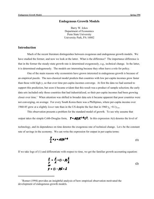
<strong>Endogenous</strong> <strong>Growth</strong> <strong>Models</strong> Spring 1996<br />
<strong>Endogenous</strong> <strong>Growth</strong> <strong>Models</strong><br />
Barry W. Ickes<br />
<strong>Department</strong> <strong>of</strong> <strong>Economics</strong><br />
<strong>Penn</strong> State University<br />
University Park, PA 16802<br />
Introduction<br />
Much <strong>of</strong> the recent literature distinguishes between exogenous and endogenous growth models. We<br />
have studied the former, and now we look at the latter. What is the difference? The importance difference is<br />
that in the former the steady-state growth rate is determined exogenously, e.g., technical change. In the latter,<br />
it is determined endogenously. The models are interesting because they <strong>of</strong>ten leave a role for policy.<br />
One <strong>of</strong> the main reasons why economists have grown interested in endogenous growth is because <strong>of</strong><br />
an empirical puzzle. The neo-classical model predicts that countries with low per-capita incomes grow faster<br />
than those with high y, so that over time per-capita incomes converge. At first the data we had seemed to<br />
support this prediction, but soon it became evident that this result was a product <strong>of</strong> sample selection; the early<br />
data sets included only those countries that had industrialized, so their per-capita incomes had been growing<br />
closer over time. 1 When attention was shifted to broader data sets it became apparent that poor countries were<br />
not converging, on average. For every South Korea there was a Phillipines, where per-capita income over<br />
1960-85 grew at a slightly lower rate than in the US despite the fact that in 1960 y p =0.1y US .<br />
This observation presents a problem for the standard model <strong>of</strong> growth. To see why assume that<br />
output takes the simple Cobb-Douglas form,<br />
In this expression A(t) denotes the level <strong>of</strong><br />
technology, and its dependence on time denotes the exogenous rate <strong>of</strong> technical change. Let s be the constant<br />
rate <strong>of</strong> savings in the economy. We can write the expression for output in per-capita terms:<br />
(1)<br />
If we take logs <strong>of</strong> (1) and differentiate with respect to time, we get the familiar growth accounting equation:<br />
(2)<br />
1 Romer (1994) provides an insightful analysis <strong>of</strong> how empirical observation motivated the<br />
development <strong>of</strong> endogenous growth models.
<strong>Endogenous</strong> <strong>Growth</strong> <strong>Models</strong> Spring 1996<br />
Equation (2) is the familiar growth accounting equation which relates growth in per-capita income to growth<br />
in the capital labor ratio (intensive growth) and growth in productivity. The coefficient $ is labor's share <strong>of</strong><br />
GNP, so it can be taken from data. Since we can measure y and k, (2) can be used to measure productivity<br />
growth.<br />
Now we can derive an expression for k$ by noting that<br />
where n is the growth rate <strong>of</strong> the<br />
labor force. Since<br />
we can write k$ as:<br />
(3)<br />
But we know from (1) that<br />
so that we can write k$ as:<br />
(4)<br />
and thus we can re-write (2) as:<br />
(5)<br />
From (5) we can see how, outside the steady state, variation in the investment rate and in y should<br />
translate into variation in the growth rate. For a broad sample <strong>of</strong> countries the value <strong>of</strong> $ is around 0.6.<br />
Recall that this is labor's share in income, given competition. This means that the exponent on y in (5) is -1.5.<br />
Now we perform the following experiment. We take a country, like the Phillipines, that had y in 1960 about<br />
0.1 that <strong>of</strong> the US. Since 0.1 -1.5 is about 30, equation (5) says that the US would have required a savings rate<br />
30 times as large as the Phillipines to grow at the same rate! If we used $ = 2/3 rather than 0.6, the required<br />
2
<strong>Endogenous</strong> <strong>Growth</strong> <strong>Models</strong> Spring 1996<br />
difference would be 100 times. The evidence clearly shows that US savings was not nearly this high relative<br />
to Phillipines.<br />
Of course this simple calculation assumes that the level <strong>of</strong> technology A(t) is the same in the two<br />
countries. Given the same A, the only way to acount for the difference in y between the countries is in the<br />
size <strong>of</strong> the capital stock. Filipino workers must be using less capital than there American counterparts,<br />
accounting for the lower per-capita incomes. From (1) it is clear that the ratio <strong>of</strong> k P to k US is 0.1 1/(1-$) , which is<br />
on the order <strong>of</strong> 0.3 percent. This implies that the marginal product <strong>of</strong> capital is much higher in the Phillipines<br />
than in the US, so a correspondingly higher investment rate is needed in the latter.<br />
The problem with this analysis is that the savings rate in the US is at most twice that <strong>of</strong> the<br />
Phillipines, not 30 or 100 times larger.<br />
To reconcile the data with the theory it is critical to somehow reduce $, so that labor is relatively less<br />
important in production. In that case diminishing returns to capital accumulation will set in much slower.<br />
The problem is to explain why the share <strong>of</strong> labor in national income is so much larger than $, or in other<br />
words, why labor is paid so much more than its marginal product while capital is paid so much less.<br />
<strong>Endogenous</strong> growth theories have developed to explain this. 2<br />
From a technical point <strong>of</strong> view, one can easily see the difference between exogenous and endogenous<br />
growth models. It is convenient to begin with the assumption <strong>of</strong> a fixed savings rate (i.e., no optimizing).<br />
Assume that output is Cobb-Douglas:<br />
(6)<br />
Net investment, dK/dt, is savings minus depreciation, so:<br />
(7)<br />
where s is the constant rate <strong>of</strong> savings. Now we are interested in 0k/k. Using the definition <strong>of</strong> 0k/k and (6):<br />
(8)<br />
Now if we multiply through by k we obtain:<br />
2 Although they are also motivated other puzzles, such as the question <strong>of</strong> why people from poor<br />
countries migrate to rich countries? Why would human capital move from where it is scarce to where it is<br />
abundant?<br />
3
<strong>Endogenous</strong> <strong>Growth</strong> <strong>Models</strong> Spring 1996<br />
(9)<br />
Our interest is in steady states, so we need an expression for 0k/k, so divide both sides <strong>of</strong> (4) by k:<br />
(10)<br />
If we take logs <strong>of</strong> both sides and differentiate with respect to time:<br />
(11)<br />
where ( k / 0k/k and we have used the fact that n, *, and s are constant in the steady state, so that their time<br />
derivatives are zero. Similarly, we have used the fact that in a steady state 0k/k is constant, hence the time<br />
derivative <strong>of</strong> the LHS <strong>of</strong> (11) is zero.<br />
Now if there are constant returns to scale in capital and labor (as in the standard model), then $ + " =<br />
1, and the last term in (11) is zero. This implies that the only steady state consistent with the model is one<br />
with zero growth. This follows since $ < 1. Notice that if there were constant returns to capital accumulation<br />
(i.e., $ = 1), then there could be steady states with ( k … 0.<br />
Of course this result has nothing to do with a fixed savings rate. In a growth model with optimizing<br />
individuals the time path <strong>of</strong> consumption will be constant if the rate <strong>of</strong> interest is equal to the rate <strong>of</strong> time<br />
preference. In a representative agent model individual and aggregate consumption coincide, so there is no<br />
growth in this case. If, on the other hand, the rate <strong>of</strong> interest exceeded the rate <strong>of</strong> time preference, there is an<br />
incentive for agents to increase consumption in the future, and thus the time path <strong>of</strong> consumption is upward<br />
sloping. Now the standard arbitrage argument suggests that the rate <strong>of</strong> interest is equal to the marginal<br />
product <strong>of</strong> capital. Hence, if the technology is such that the marginal product <strong>of</strong> capital goes to zero as capital<br />
per worker increases, it follows that the rate <strong>of</strong> interest will eventually equal the rate <strong>of</strong> time preference. At<br />
this point desired consumption is constant over time and the process <strong>of</strong> capital accumulation stops.<br />
Jones and Manuelli (1990) point out that for growth to be possible the marginal product <strong>of</strong> capital<br />
must be bounded from below. That is, as k goes to infinity, f'(k) goes to some lower bound, B. If this is the<br />
case, and if B > than the rate <strong>of</strong> time preference, then continuous growth is feasible.<br />
4
<strong>Endogenous</strong> <strong>Growth</strong> <strong>Models</strong> Spring 1996<br />
To make this clearer, note that from (10) we can write the growth rate <strong>of</strong> capital, ( k , as:<br />
(12)<br />
For ( k > 0 in steady state, it must be the case that<br />
This implies, in turn, that<br />
is necessary and sufficient for a steady state with positive growth. By l’Hopital’s rule:<br />
(15)<br />
where the inequalities results from the condition for ( k to be positive. But (13) clearly violates the Inada<br />
conditions, since f’(k) goes to zero as k goes to infinity. Thus standard production functions are inconsistent<br />
with endogenous growth.<br />
To remedy this situation, Jones and Manuelli suggest we consider production functions <strong>of</strong> the type<br />
(16)<br />
which implies that<br />
so that (13) is satisfied. Notice that with the Jones-Manuelli bound, as k goes to infinity f k goes to b > 0.<br />
Production functions that resemble (14) have display diminishing returns to capital, up to a point. Thus such<br />
an economy will display transition dynamics, and it will display positive growth in the steady state. 3<br />
Notice that convex technologies can be consistent with such a bound. A convex technology requires<br />
that f'(k) be a decreasing function <strong>of</strong> k, but not that it decrease without bound. A simple example would be a<br />
production function <strong>of</strong> the form: F(K, L) = AK " L 1-" + bK. Of course this example is not all that appealing<br />
since it implies that labor's share <strong>of</strong> national income goes to zero.<br />
3<br />
As long as .<br />
5
<strong>Endogenous</strong> <strong>Growth</strong> <strong>Models</strong> Spring 1996<br />
The essence <strong>of</strong> endogenous growth models is to somehow implement a Jones-Manuelli bound on the<br />
marginal product <strong>of</strong> capital. In essence, what the endogenous growth models do is impose constant returns on<br />
the reproducible factors <strong>of</strong> production (i.e. $ = 1). This kind <strong>of</strong> model gives no role to non-reproducible<br />
factors <strong>of</strong> production, such as land and labor, and gives primary focus to capital. We shall examine this model<br />
(Rebelo's model) shortly. Note that the model is not ignoring labor per se, but labor devoid <strong>of</strong> human capital.<br />
The implied production function is<br />
(17)<br />
The idea here is that the labor force improves in quality with human capital accumulation, and that savings is<br />
devoted to both. Human and physical capital are combined together in a broad measure, and a production<br />
function like (15) above results. This is the Lucas-Uzawa approach.<br />
An alternative possibility is to assume that there exist increasing returns to scale. If n = 0, we can<br />
have non-reproducible inputs (" > 0), and steady state growth, ( k > 0, if there are constant returns to the<br />
inputs that can be accumulated ($ = 1). But this means that there are increasing returns to scale " + $ > 1.<br />
Notice that with increasing returns to scale we have some additional problems that arise because we<br />
cannot have competitive prices. There are two main ways to get around this problem. The first (originally<br />
due to Marshall, and is now associated with Romer via Arrow) is to assume IRS at the aggregate level, but to<br />
assume CRS at the firm level. The idea is that there are spillovers that are external to the firm, but that none<br />
<strong>of</strong> the firms take them into account. Hence all the firms face "concave" problems, but the economy as a<br />
whole faces an IRS production function which can generate endogenous growth. It is immediately apparent<br />
from this description that the equilibria in such a model will not be efficient.<br />
The (Cobb Douglas) production function is<br />
(18)<br />
where K t is private capital and 6 t is aggregate capital in the economy. Individuals firms assume that they<br />
cannot affect the aggregate stock <strong>of</strong> capital, so they take 6 as given. This makes the firm's problem quite<br />
standard. But in the aggregate, ' i K ti = 6 t . Thus the aggregate production function will be<br />
(19)<br />
Now examine (11) in the context <strong>of</strong> (13). Since (11) is derived from the aggregate production<br />
function, we replace $ in (11) with $' / $ + R. Now if $' = 1, then we can have steady state growth. Hence<br />
we have constant returns to capital in an increasing returns to scale world. The reason is that the spillover is<br />
external to the firm. Modelling externalities in this way we get around the problem <strong>of</strong> in-existence <strong>of</strong><br />
competitive equilibrium. But the equilibria will be non-optimal. In the Romer model these externalities take<br />
the form <strong>of</strong> knowledge spillovers, as we shall see.<br />
6
<strong>Endogenous</strong> <strong>Growth</strong> <strong>Models</strong> Spring 1996<br />
An alternative way to get around the problem <strong>of</strong> existence <strong>of</strong> competitive equilibrium with IRS is to<br />
drop the assumption <strong>of</strong> competitive behavior. With imperfect competition factor returns do not exhaust total<br />
output. Hence there are rents that can be assigned to activities that are not directly productive, but may<br />
contribute to the expansion <strong>of</strong> the frontiers <strong>of</strong> knowledge such as research and development. Many<br />
economists believe that this is an important source <strong>of</strong> economic growth.<br />
There have also been models that include both externalities and imperfect competition (e.g.,<br />
Grossman and Helpman). In these models firms undertake R&D in order to introduce new goods (a product<br />
differentiation motive), but this activity also increases the general stock <strong>of</strong> knowledge. This, in turn, makes it<br />
less costly to undertake further research (which insures that it will continue) and it increases the productivity<br />
<strong>of</strong> other inputs. Since the stock <strong>of</strong> knowledge grows at a constant rate, so does output.<br />
<strong>Endogenous</strong> <strong>Growth</strong> <strong>Models</strong><br />
Before looking at some specific models in more detail it is worthwhile to look again at the distinction<br />
between endogenous and exogenous growth models. We have seen that the key to the former was the<br />
inexistence <strong>of</strong> diminishing returns to the inputs that can be accumulated. Hence the return to investment in all<br />
these models end up being a constant, A*:<br />
(1)<br />
Let us further suppose that consumption is determined according to an intertemporal optimization<br />
problem, so that the MGR results. We will derive this again shortly (see equation (18) below). Since our<br />
concern is with endogenous growth models, rather than let the growth rate be n, we denote it by ( k , which is<br />
constant in the steady state: 4 (2)<br />
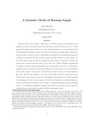
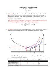
We have two equations in r and ( k , so we can plot this as in figure 1. Notice that the<br />
intersection <strong>of</strong> the two curves yields the equilibrium growth rate. Suppose that A* increases. Then it is<br />
apparent from the figure that ( k will increase. Hence the focus <strong>of</strong> attention in endogenous growth models is<br />
to understand the determinants <strong>of</strong> A*. In particular, concern centers on the role <strong>of</strong> policy in affecting A*. 5<br />
4 Notice from (8), below, we have r = D + F(. Hence let F = 1, and we have expression (2).<br />
5 Less attention is devoted to the determinants <strong>of</strong> D, or <strong>of</strong> the inter-temporal elasticity <strong>of</strong> consumption<br />
(the inverse <strong>of</strong> which multiplies ( k , but which I have assumed to be unity). One might consider, however,<br />
that some countries are more willing to defer consumption than others. This has been relatively<br />
unstudied, however.<br />
7
<strong>Endogenous</strong> <strong>Growth</strong> <strong>Models</strong> Spring 1996<br />
Figure 1<br />
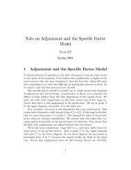
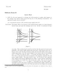
Now we contrast this with the exogenous growth model. In this case we still have equation (2), but<br />
now the growth rate is exogenous. Hence we have figure 2. Comparing the two pictures we see that in the<br />
exogenous growth model, a change in any <strong>of</strong> the parameters that determine the return to consumption affect<br />
r*, but not the growth rate. In the endogenous growth model such changes affect the growth rate, but not the<br />
interest rate.<br />
Rebelo's Model<br />
The simplest introduction into this literature is Rebelo's model. Rebelo assumes that the production<br />
function is linear in the only input, capital. Hence there are constant returns to scale and constant returns to<br />
capital. The production function is:<br />
(3)<br />
where A is an exogenous constant, and K is aggregate capital broadly defined. Thus K can include not just<br />
physical capital but also human capital as well as the stock <strong>of</strong> knowledge and even financial capital.<br />
8
<strong>Endogenous</strong> <strong>Growth</strong> <strong>Models</strong> Spring 1996<br />
Figure 2<br />
For simplicity we assume that n = * = 0. The utility function that households maximize is <strong>of</strong> the<br />
constant intertemporal elasticity <strong>of</strong> substitution form:<br />
(4)<br />
where D is the rate <strong>of</strong> time preference and F -1 is the intertemporal elasticity <strong>of</strong> substitution. Let b be the<br />
financial wealth <strong>of</strong> households. Financial wealth is physical capital plus bonds. In the aggregate the net<br />
supply <strong>of</strong> bonds equals zero, so b = k. Households thus face a financial constraint <strong>of</strong> the form:<br />
(5)<br />
Agents maximize (4) subject to (5) and appropriate boundary conditions. The Hamiltonian for the<br />
problem is:<br />
9
<strong>Endogenous</strong> <strong>Growth</strong> <strong>Models</strong> Spring 1996<br />
(6)<br />
where v is the multiplier on the costate variable, and I have used A = r. 6 The first-order conditions for this<br />
problem include:<br />
(7)<br />
and a transversality condition.<br />
Now take logs <strong>of</strong> (i) and differentiate with respect to time to get<br />
(8)<br />
where ( is the balanced growth rate <strong>of</strong> consumption (and capital). Note that (ii) implies that v0/v = -A, so that<br />
from (8) it follows that -A = -D - F(. Hence<br />
6 Alternatively, we could write the present value Hamiltonian as:<br />
where q t = ve -Dt , is the current value <strong>of</strong> the costate variable. The F.O.C. are then<br />
Note that -H b is equal to -q t Ae -Dt , so that the second condition can be written as:<br />
Now we can substitute for q t from the first condition, and we obtain:<br />
which is equation (9) in the text.<br />
10
<strong>Endogenous</strong> <strong>Growth</strong> <strong>Models</strong> Spring 1996<br />
(9)<br />
Note that (9) implies that A = F( + D, which is the MGR (recall that f'(k t ) = A in this model). This is just the<br />
curve rc in figure 1.<br />
What about k0? If we substitute k = b into (5) we have k0 = Ak - c. Divide both sides by k, and note<br />
that in a steady state k0/k is constant. Then if we take logs <strong>of</strong> both sides and differentiate with respect to time<br />
we obtain c0/c = k0/k. Note from (9), however, that this balanced growth rate need not be zero. As long as A is<br />
large enough, we will have positive steady state growth.<br />
Now let us look at the interaction <strong>of</strong> the savings rate and the rate <strong>of</strong> growth. We have:<br />
(10)<br />
Hence the growth rate <strong>of</strong> an economy depends on its savings rate and on the productivity <strong>of</strong> its technology,<br />
since (10) implies that ( = (s/y)A. Furthermore, the last equality in (10) implies that s/y depends on D and F. 7<br />
If D is small, society is more patient, and savings and the growth rate will be higher. Similarly if agents are<br />
more willing to substitute consumption intertemporally, F low, then again savings and growth will be higher.<br />
What remains to be explained is the determination <strong>of</strong> A, which we shall discuss in the context <strong>of</strong> the Romer<br />
and Lucas models.<br />
Note also that this model does not predict convergence. To see this assume that countries have the<br />
same parameters, (A, F, D), but that they start with different initial capital stocks. Since they grow at the same<br />
rates (by virtue <strong>of</strong> (10)), their levels <strong>of</strong> per-capita income cannot converge. What is perhaps <strong>of</strong> more interest,<br />
is that given identical preferences, different values <strong>of</strong> A imply different growth rates, so that if poor counties<br />
have low A, they will not catch up. This seems to imply a role for policy in economic development, if it can<br />
affect A. We now must turn to its determination.<br />
Romer's Model<br />
Romer started the endogenous growth literature by considering a model with increasing returns to<br />
scale at the economy-wide level, but constant returns to scale at the firm level. The model then supports a<br />
competitive equilibrium, but this equilibrium is non-optimal. A higher growth rate could be achieved if the<br />
7<br />
And, <strong>of</strong> course, on A which determines the rate <strong>of</strong> return.<br />
11
<strong>Endogenous</strong> <strong>Growth</strong> <strong>Models</strong> Spring 1996<br />
externality associated with investment could be internalized. This alone made the model popular, and it has<br />
spawned a large literature.<br />
Romer follows Arrow's seminal work on the economics <strong>of</strong> learning by doing. Arrow noted from case<br />
studies that there was strong evidence that experience and increasing productivity were associated. He argued<br />
that a good measure <strong>of</strong> increase in experience is investment, because "each new machine produced and put<br />
into use is capable <strong>of</strong> changing the environment in which production takes place, so that learning takes place<br />
with continuous new stimuli" (157). Arrow then indexes experience by cumulative investment.<br />
Let the production function for firm i be:<br />
(11)<br />
where A(t) is reflects the stock <strong>of</strong> knowledge at time t. The idea is that labor is more productive given the<br />
accumulation <strong>of</strong> knowledge. This, in turn, depends on experience which is a function <strong>of</strong> past investment <strong>of</strong><br />
all firms in the economy. Hence:<br />
(12)<br />
with no depreciation, the sum <strong>of</strong> past investment is equal to the aggregate capital stock. The learning by<br />
doing assumption is that A(t) = G(t) 0 , with 0 < 1. This means that investment raises the productivity <strong>of</strong> labor,<br />
but at a decreasing rate. Hence we can rewrite (11) as:<br />
(13)<br />
Notice that (13) is constant returns to scale holding 6 fixed, but that it is increasing returns to scale when we<br />
consider the three "inputs" at the same time. With a large number <strong>of</strong> firms we can assume that firms take 6 as<br />
given in their maximization problem. This will be the source <strong>of</strong> the externality. A command planner would<br />
consider the effect <strong>of</strong> investment on production via the experience gained. A firm will not.<br />
If we aggregate across firms we can write the aggregate production function as:<br />
(14)<br />
Dividing through by L gives us a per-capita production function:<br />
(15)<br />
where k = K/L, and y = Y/L. Assume that the households maximize a utility function as in (4), subject to a<br />
dynamic constraint (again ignoring population growth):<br />
(16)<br />
To obtain the conditions <strong>of</strong> the competitive equilibrium we set up the household's decision, as before,<br />
but remembering that the household chooses k assuming that 6 is given. The Hamiltonian for this problem is<br />
12
<strong>Endogenous</strong> <strong>Growth</strong> <strong>Models</strong> Spring 1996<br />
(17)<br />
and the first order conditions will include:<br />
(18)<br />
Equilibrium in the capital market requires that 6 = Lk. Now if we take logs <strong>of</strong> (18i) and differentiate with<br />
respect to time we get<br />
(19)<br />
Now substitute for v0/v from (27ii), using 6 = Lk, and we obtain:<br />
(20)<br />
Expression (20) relates the growth <strong>of</strong> consumption to the difference between the marginal product <strong>of</strong> capital<br />
and the discount rate, times the factor <strong>of</strong> proportionality, F -1 . Now divide both sides <strong>of</strong> (16) by k, take logs<br />
and time derivatives, and we can show that k0/k = (. Note that this model has the counterfactual implication<br />
that the growth rate <strong>of</strong> consumption is increasing in the population, L. This is due to the nature <strong>of</strong> the scale<br />
effect. If we had related experience to the average capital stock instead, then this would not occur.<br />
How do we interpret these results? Let $L 0 = A*. Then if $ + 0 = 1, (20) reduces to<br />
(21)<br />
which is isomorphic to Rebelo's model (equation (9)), except that in this case the social and private marginal<br />
products <strong>of</strong> capital are unequal. Thus Romer's model also generates endogenous growth, when $ + 0 = 1.<br />
This would not be true, however, if $ + 0 < 1. In this case the model is identical to the standard<br />
exogenous growth model. In the context <strong>of</strong> (6), we would have<br />
in place <strong>of</strong> $ as capital's share in<br />
(6). But then the only steady state would be the one with ( = 0. This is an important point. It means that<br />
increasing returns are not a sufficient condition for endogenous growth. What we need is sufficiently large<br />
increasing returns so that $ + 0 = 1.<br />
Now let us consider what the growth rate would be if a planner were to choose levels <strong>of</strong> investment.<br />
This is important since we know that private agents are not considering the spillover that arises from<br />
13
<strong>Endogenous</strong> <strong>Growth</strong> <strong>Models</strong> Spring 1996<br />
investment. Recall that 6 = Lk. Hence we could rewrite the last term in the Hamiltonian as v(k $ + 0 L 0 - c).<br />
Consequently we can rewrite (20) as:<br />
(23)<br />
since 0 > 0, this is clearly greater than the growth rate in the competitive equilibrium. This is clearly due to<br />
the failure <strong>of</strong> private agents to take into account the effects <strong>of</strong> their investment on aggregate capital, and hence<br />
on learning by doing. Private agents fail to internalize the spillover in production; they under-invest, and,<br />
therefore, they "undergrow."<br />
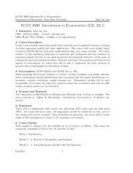
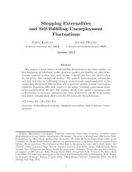
Figure 3<br />
It is instructive to put this in terms <strong>of</strong> a figure similar to 1. First note that in competitive equilibrium<br />
firms invest until the marginal product <strong>of</strong> capital is equal to r. Since the production function is<br />
(24)<br />
the private marginal product is $k $ - 1 k 0 L 0 = $k $ + 0 - 1 L 0 , due to the failure <strong>of</strong> private agents to consider the<br />
effect <strong>of</strong> investment on 6. But for the planner the relevant marginal product is<br />
(25)<br />
which is clearly larger if 0 > 0. Hence in terms <strong>of</strong> figure 3, the r* = A line for the planner (ri planner ) lies above<br />
that for the competitive equilibrium. But this clearly gives a lower equilibrium rate <strong>of</strong> growth in the latter<br />
case.<br />
14
<strong>Endogenous</strong> <strong>Growth</strong> <strong>Models</strong> Spring 1996<br />
But it is not just the fact that the competitive equilibrium and the solution to the planners problem<br />
differ that is interesting. The model also allows one to introduce significant effects from policy. Suppose, for<br />
example, that tax laws are changed that increase the incentive to invest (an ITC for example). In the standard<br />
approach this may have some effect on the efficiency <strong>of</strong> the allocation <strong>of</strong> resources, and hence effect the level<br />
<strong>of</strong> income today, but it will leave the growth rate unaffected. In this model, on the other hand, an increase in<br />
investment incentives will shift ri upwards, and hence raise (. This is clearly optimal as long as the new ri ce<br />
does not lie above ri planner in figure 3.<br />
There is still more to the point, however, if we think about a case where the effect <strong>of</strong> a policy is to<br />
raise the growth rate and lower the level <strong>of</strong> output. Now if we consider a long time horizon, growth rate<br />
effects will dominate level effects. Romer gives the following numerical example, which stems from<br />
Jorgenson's evaluation <strong>of</strong> the effects <strong>of</strong> the 1986 tax reform.<br />
Suppose that elimination (say by the 1986 tax reform) <strong>of</strong> ITC and uniform taxing <strong>of</strong> capital gains and<br />
dividend income reduces distortions and raises the level <strong>of</strong> output by 1% (forever). Suppose that interest rates<br />
were 5% and that the growth rate <strong>of</strong> output was 3%. The present value <strong>of</strong> future GNP is 1.0/(0.05 - 0.03) =<br />
1.0/0.02 = 50 times current GNP. Now suppose that the level <strong>of</strong> GNP rises by 1%, and that growth is<br />
exogenous (and hence unchanged). The present value <strong>of</strong> future GNP rises to 1.01/.02 = 50.5 times pre-reform<br />
GNP. So the effect <strong>of</strong> the tax reform is to increase wealth by half a year's GNP. Now suppose that the tax<br />
reform also effects the growth rate, reducing it from 3% to 2.9%. The effect <strong>of</strong> the policy then is to make the<br />
present value <strong>of</strong> future GNP 1.01/(.05 - .029) = 1.01/.021 = 48.1 times current GNP. So output falls by 2<br />
years worth <strong>of</strong> output . It is not surprising that growth rate effects dominate level effects, and that is the main<br />
point <strong>of</strong> the example. It is instructive to see that the assumption that the growth rate will be unaffected can<br />
have serious implications for the evaluation <strong>of</strong> policy.<br />
Many people relate endogenous growth to increasing returns to scale. This is, to a large extent, due to<br />
the fact that Romer's model really got this literature going. 8 But it is clear from even our brief survey, that<br />
increasing returns are neither necessary, nor sufficient to generate endogenous growth. The former statement<br />
follows from Rebelo's model which generates endogenous growth without increasing returns. The latter<br />
statement follows from Romer's model, since we have seen that for endogenous growth to be possible, we<br />
need sufficiently large externalities.<br />
8 Although Romer recognized this point, many still took increasing returns to be the central lesson <strong>of</strong><br />
the model.<br />
15
<strong>Endogenous</strong> <strong>Growth</strong> <strong>Models</strong> Spring 1996<br />
A Simple Human Capital Model<br />
Let us begin by examining a simple human capital model. We really should exmaine a two-secotr<br />
model, but instead we will assume that output can be used for human and physical capital. There is constant<br />
returns to scale for both inputs. Our assumptions about production and output can be written as:<br />
(1)<br />
with the following accumulation conditions:<br />
(2)<br />
Notice that in (2) we have assumed that the rate <strong>of</strong> depreciation <strong>of</strong> the human and physical capital stock are<br />
equal. This is not essential, but it radically simplifies the following.<br />
We can write the present value Hamiltonian as:<br />
(3)<br />
If we use standard CARRA utility, and appropriate nonnegativity conditions, I K , I H $ 0<br />
(which we will ignore for a bit), we obtain from the FONC the conditions for the growth <strong>of</strong> consumption:<br />
(5)<br />
where we note that the first two terms inside the brackets <strong>of</strong> (4) is the net marginal product <strong>of</strong> physical capital.<br />
Since agents can invest in physical and human capital, and since the cost (in terms <strong>of</strong> output is the<br />
same), it follows that the net marginal product <strong>of</strong> physical capital should equal the net marginal product <strong>of</strong><br />
human capital. The net marginal product <strong>of</strong> human capital is<br />
. Thus, setting the<br />
two equal yields:<br />
16
<strong>Endogenous</strong> <strong>Growth</strong> <strong>Models</strong> Spring 1996<br />
(7)<br />
which implies that:<br />
(8)<br />
Given the structure <strong>of</strong> the model (6) makes perfect sense. Households can save in either physical or human<br />
forms, and the proportions in which they do this must be related to the relative productivity <strong>of</strong> the two<br />
activities. Notice that (6) also implies that in the steady state the ratio <strong>of</strong> physical to human capital will be<br />
constant.<br />
Using (6) in the expression for the MP K we can write the rate <strong>of</strong> return to investment, r*, as:<br />
(9)<br />
Clearly r* is constant because <strong>of</strong> the constant returns to scale with respect to physical and human capital.<br />
Note further that if K/H is constant then ( c , the steady-state growth rate <strong>of</strong> consumption,is constant and equal<br />
to:<br />
(10)<br />
It is interesting to note that if we substitute from (6) into the production function (1) we obtain an<br />
expression that is clearly <strong>of</strong> the AK type:<br />
(11)<br />
From (9) it is clear that for any given value <strong>of</strong> " this is an AK model.<br />
17
<strong>Endogenous</strong> <strong>Growth</strong> <strong>Models</strong> Spring 1996<br />
What happens if the initial ratio <strong>of</strong> physical to human capital, , differs from ?<br />
Instantaneous adjustment makes no sense. An economy cannot turn K into H overnight. This would require<br />
an infinite rate <strong>of</strong> investment, and if the initial physical capital stock was too high, an infinitely negative rate<br />
<strong>of</strong> investment, which is clearly nonsense.<br />
Suppose that human capital is initially too abundant, i.e.,<br />
then households wish to reduce H relative to K, so I H =0. Human capital depreciates at rate *, by assumption,<br />
so<br />
, or . This implies that<br />
(16)<br />
where I H = 0. Notice that this is much like the Solow model, except that instead <strong>of</strong> population growth, n, we<br />
have . Now as , eventually we have .<br />
Once we reach the proper ratio <strong>of</strong> K to H, then investment in human capital can resume, and we<br />
return to the original solution with (* > 0. So the dynamics <strong>of</strong> the neoclassical model applies when H is<br />
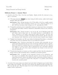
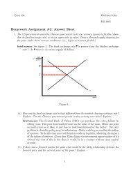
abundant, and the K-H solution applies when we get to the steady state. In the transition, and decline<br />
monotonically over time. The marginal product <strong>of</strong> capital declines over time, but it is still greater than the<br />
marginal product <strong>of</strong> human capital until we reach . The dynamics thus resemble:<br />
18
<strong>Endogenous</strong> <strong>Growth</strong> <strong>Models</strong> Spring 1996<br />
Y &<br />
Y<br />
due to W W 2<br />
perhaps<br />
α<br />
1 − α<br />
due to Black<br />
Death, perhaps<br />
K<br />
H<br />
As drawn in figure 4 adjustment is symmetric when the K/H ratio is wrong , but there is no reason<br />
why this must be so. One could add asymmetry; presumably it is harder to accumulate H than K. For both<br />
you need to save, but you need H to produce H. If so then the curve might be flatter to the right <strong>of</strong> the proper<br />
K/H. That is, when K is abundant the change in output is smaller than when H is abundant.<br />
But to really deal with this analysis we need a two-sector model.<br />
Lucas's Human Capital Model<br />
Lucas's paper on the "Mechanics <strong>of</strong> Economic Development" develops a model in which constant<br />
returns to scale in the inputs that can be accumulated is obtained by arguing that all inputs can be<br />
accumulated. Rather than rely on externalities, as in Romer, Lucas introduces human capital, rather than<br />
physical labor, in the production function. Agents invest in human capital through their "studies." All inputs<br />
<strong>of</strong> the production function can thus be accumulated. With a CRS production function, we have essentially<br />
Rebelo's model, where the broad measure <strong>of</strong> capital includes human and physical capital. <strong>Growth</strong> is then<br />
generated by assuming that the incentive to invest in human capital is nondecreasing in human capital. That<br />
is, Lucas postulates a production function <strong>of</strong> human capital which is constant returns to scale in human<br />
19
<strong>Endogenous</strong> <strong>Growth</strong> <strong>Models</strong> Spring 1996<br />
capital. Hence the marginal product <strong>of</strong> human capital -- which determines the incentive to spend time<br />
studying -- is constant.<br />
Let u be the fraction <strong>of</strong> non-leisure time agents spend working (i.e., producing the output good Y),<br />
and let h be a measure <strong>of</strong> the average quality <strong>of</strong> workers and L be the number <strong>of</strong> bodies. Then uhL is to the<br />
total effective labor force. Population is going to grow at rate n, and is not important. Hence we let n = 1 and<br />
write the production function in per-capita terms. We can write the production function as:<br />
(1)<br />
where the term uh is <strong>of</strong>ten called human capital. This production function clearly exhibits constant returns to<br />
scale in k and uh, since doubling these inputs doubles output. Note that if we interpret k $ [uh] (1 - $) as being a<br />
broad measure <strong>of</strong> capital, we are back to Rebelo's model (providing that the incentive to accumulate human<br />
capital does not decrease over time; otherwise we would cease accumulating it). Consequently this is<br />
sufficient to generate endogenous growth. We could stop here.<br />
Lucas chooses to introduce, however, an externality in human capital to reflect the fact that people are<br />
more productive when they are around clever people (some people seem to be less productive in such<br />
situations, but that is another story). Let h a be the average level <strong>of</strong> human capital in the labor force. Then we<br />
can write the production function as:<br />
(2)<br />
R<br />
where h a represents the externality from average human capital. This externality is introduced, not to obtain<br />
endogenous growth (we have seen already that this is not needed), but to obtain some extra results on<br />
migration across countries. 9 In any event, agents choose to maximize the standard intertemporal utility<br />
function subject to the capital accumulation constraint:<br />
(3)<br />
To complete the model we need to specify how knowledge is accumulated. There are two ways to<br />
think about this. First, agents learn when they study! Thus we would relate human capital accumulation to<br />
9 It is a bit strange to have the externality depend on average human capital. This seems to imply that<br />
if an agent with lower than average human capital migrates to the US everyone else becomes less<br />
productive!<br />
20
<strong>Endogenous</strong> <strong>Growth</strong> <strong>Models</strong> Spring 1996<br />
time spend not working. Second, agents accumulate human capital through on the job training; this would<br />
relate to time working. For now we consider only the former approach:<br />
(4)<br />
Notice that (4) implies constant returns to scale in human capital accumulation, since h0/h is proportional to<br />
study time. This assumption is crucial. It is the driving force behind sustained growth in the model.<br />
Let us now consider the agents problem. The representative agent chooses a stream <strong>of</strong> consumption<br />
and the time spend studying, taking h a as given. The constraints are the asset accumulation equation (3) and<br />
the "study-time" equation (4). The Hamiltonian is<br />
(5)<br />
The F.O.C. (with respect to C, u, k, and h, respectively) are:<br />
(6)<br />
Note, <strong>of</strong> course, that h a = h, although agents ignore their own effect on it.<br />
As before, take logs and derivatives <strong>of</strong> (i), and use (iii) and h a = h to obtain:<br />
(7)<br />
Now lets show that the growth rate <strong>of</strong> consumption is equal to the growth rate <strong>of</strong> capital. Divide both<br />
sides <strong>of</strong> (3) by k to get<br />
(8)<br />
Comparing (8) with (7) it is apparent that the first part <strong>of</strong> the first term on the rhs <strong>of</strong> (8) is equal to ((F + D)/$.<br />
Hence if we take logs and derivative <strong>of</strong> both sides <strong>of</strong> (8), this term will drop out since all <strong>of</strong> its elements are<br />
21
<strong>Endogenous</strong> <strong>Growth</strong> <strong>Models</strong> Spring 1996<br />
constants. Thus we will get c0/c = ( =<br />
= ( k . This leaves one more growth rate to go: the growth rate <strong>of</strong><br />
human capital, (/ ( h ).<br />
Take (7) and move all the constants to the left hand side. We obtain:<br />
(11)<br />
If we take logs and derivatives <strong>of</strong> both sides the LHS will be zero, <strong>of</strong> course, and we get:<br />
(12)<br />
which we can re-arrange to obtain:<br />
(13)<br />
from which we can see that, in the absence <strong>of</strong> the human capital externality, ( = ( h .<br />
we can write<br />
Now we must determine the value <strong>of</strong> ( or ( h as a function <strong>of</strong> the parameters <strong>of</strong> the model. From (6ii)<br />
(14)<br />
Now, once again, take logs and derivatives <strong>of</strong> both sides to get<br />
(15)<br />
We can easily get an expression for v0/v from (6iii):<br />
(16)<br />
where the last equality follows from (9).<br />
22
<strong>Endogenous</strong> <strong>Growth</strong> <strong>Models</strong> Spring 1996<br />
we obtain:<br />
Now to find the value <strong>of</strong> 80 /8 divide both sides (6iv) by 8, and then substitute for v/ 8 from (12), and<br />
(17)<br />
which means that the shadow price <strong>of</strong> human capital is decreasing at the constant rate, N, which is the<br />
productivity parameter <strong>of</strong> the "studying technology."<br />
Finally, we substitute (10) and (11) into (9) and use the result from (7) to substitute for ( and we<br />
obtain:<br />
(18)<br />
Notice that if there is no human capital externality, R = 0, and thus we find that ( = ( h = (N - D)/F. With N =<br />
A this is the same growth rate as in the Rebelo model. Note the implication; if the production <strong>of</strong> human<br />
capital improves (i.e., N increases) the growth rate increases. So the productivity <strong>of</strong> human capital<br />
accumulation affects growth. The policy implications are clear.<br />
When the human capital externality is present the competitive solution differs from the command<br />
optimum. The planners' problem would internalize the externality, since now the effect <strong>of</strong> the choice <strong>of</strong> h on<br />
h a would be taken into account. Rewrite the Hamiltonian and perform the usual substitutions to derive:<br />
(19)<br />
which is higher than the market solution, if F -1 is not too big. If the elasticity <strong>of</strong> substitution (F -1 ) is too big<br />
then agents are unwilling to defer consumption, and this overcomes the external benefits that the planner is<br />
taking into account. When F -1 is not too big then the private return to studying is lower than the social<br />
return, so agents (in the decentralized solution) will not invest in human capital as much as would be socially<br />
optimal.<br />
23
<strong>Endogenous</strong> <strong>Growth</strong> <strong>Models</strong> Spring 1996<br />
A Model With Public Goods (Barro)<br />
Barro considers a model where public expenditure is productive. It is easy to think <strong>of</strong> investments in<br />
infrastructure that make private production more pr<strong>of</strong>itable.<br />
Let G be aggregate services, then g = G/N is the quantity allocated to each <strong>of</strong> n producers. Notice<br />
that this is not exactly what we usually think <strong>of</strong> as a public good, since it is rival and excludable. We could<br />
think <strong>of</strong> infrastructure such as phone lines or roads to factories. In any event, this allows us to write the<br />
production function:<br />
(1)<br />
Notice that y is subject to diminishing returns to k, but not to k and g. The individual producer takes g as<br />
fixed (i.e., independent <strong>of</strong> his decision about k).<br />
The government runs a balanced budget; hence J = g/y. Since g uses one unit <strong>of</strong> the single output<br />
good, efficiency requires g* such that My/Mg* = 1. Now if g is set efficiently, then from (1) it follows that g/y<br />
= ". This follows because<br />
(2)<br />
Now the marginal product <strong>of</strong> capital, determined from (1) is<br />
(3)<br />
where the last equality follows if g = g*.<br />
The private return to investment is what is left after taxes:<br />
(4)<br />
We can substitute the RHS <strong>of</strong> (4) into the Rebelo equation to solve for the growth rate <strong>of</strong> the economy.<br />
Notice that with J = 0 social and private returns are equal. Otherwise, the private return to investment is less<br />
than the social, because entrepreneurs do not consider the effect they have on others through investment. The<br />
24
<strong>Endogenous</strong> <strong>Growth</strong> <strong>Models</strong> Spring 1996<br />
channel is that with higher investment, and thus income, there is more government spending, which, since it is<br />
productive, makes for higher growth. But individual investors do not take into account the effect on y from<br />
their investments.<br />
Concluding Note<br />
These notes are an introduction to the literature on endogenous growth models. This literature is<br />
exploding, so it is not possible to be comprehensive. The purpose <strong>of</strong> these notes is to develop the basic<br />
structure <strong>of</strong> these models, and to make it clear how they obtain results so different from exogenous growth<br />
models.<br />
There is one important lacuna in these notes. I have not covered models that generate endogenous<br />
growth via the introduction <strong>of</strong> new products. This literature is important, and its absence here should not be<br />
taken to imply any judgment about these models. I hope to remedy this defect in the next edition <strong>of</strong> these<br />
notes.<br />
25
<strong>Endogenous</strong> <strong>Growth</strong> <strong>Models</strong> Spring 1996<br />
References<br />
Barro, R., "Government Spending in a Simple Model <strong>of</strong> <strong>Endogenous</strong> <strong>Growth</strong>," Journal <strong>of</strong> Political Economy,<br />
98, 1990, S103-S125.<br />
Jones, L., and R. Manuelli, "A Convex Model <strong>of</strong> Equilibrium <strong>Growth</strong>: Theory and Policy Implications,"<br />
Journal <strong>of</strong> Political Economy, 98, 5, 1990, 1008-1038.<br />
Lucas, R.E., "On the Mechanics <strong>of</strong> Economic Development," Journal <strong>of</strong> Monetary <strong>Economics</strong>, 22, 1988: 3-<br />
42.<br />
Rebelo, S., "Long-Run Policy Analysis and Long-Run <strong>Growth</strong>," Journal <strong>of</strong> Political Economy, 99, 500-521.<br />
Romer, P., "Increasing Returns and Long-Run <strong>Growth</strong>," Journal <strong>of</strong> Political Economy, 94, 1986, 1002-1037.<br />
Sala-i-Martin, X., "Lecture Notes on Economic <strong>Growth</strong>: Five Prototype <strong>Models</strong> <strong>of</strong> <strong>Endogenous</strong> <strong>Growth</strong>,"<br />
Yale University, December 1990.<br />
26