Open channel flows
Open channel flows
Open channel flows

Create successful ePaper yourself
Turn your PDF publications into a flip-book with our unique Google optimized e-Paper software.
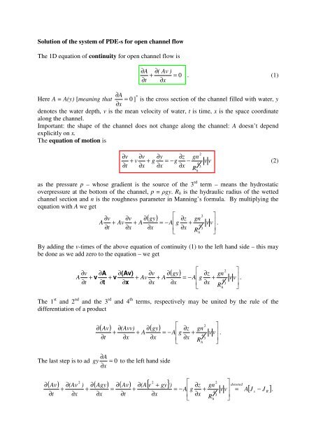
Solution of the system of PDE-s for open <strong>channel</strong> flow<br />
The 1D equation of continuity for open <strong>channel</strong> flow is<br />
∂A<br />
∂(<br />
Av )<br />
+ = 0<br />
∂t<br />
∂x<br />
. (1)<br />
∂A<br />
Here A = A(y) [meaning that = 0 ] * is the cross section of the <strong>channel</strong> filled with water, y<br />
∂x<br />
denotes the water depth, v is the mean velocity of water, t is time, x is the space coordinate<br />
along the <strong>channel</strong>.<br />
Important: the shape of the <strong>channel</strong> does not change along the <strong>channel</strong>: A doesn’t depend<br />
explicitly on x.<br />
The equation of motion is<br />
∂v<br />
∂v<br />
∂y<br />
+ v + g<br />
∂t<br />
∂x<br />
∂x<br />
∂z<br />
gn<br />
= −g<br />
−<br />
∂x<br />
R<br />
2<br />
4<br />
3<br />
h<br />
v v<br />
(2)<br />
as the pressure p – whose gradient is the source of the 3 rd term – means the hydrostatic<br />
overpressure at the bottom of the <strong>channel</strong>, p = ρgy. R h is the hydraulic radius of the wetted<br />
<strong>channel</strong> section and n is the roughness parameter in Manning’s formula. By multiplying the<br />
equation with A we get<br />
⎡<br />
2<br />
∂v<br />
∂v<br />
∂ gy ∂z<br />
gn<br />
⎤<br />
A<br />
∂t<br />
+ Av + A<br />
∂x<br />
( )<br />
∂x<br />
= −A⎢g<br />
+<br />
⎢ ∂x<br />
⎣ R<br />
4<br />
3<br />
h<br />
v v⎥<br />
.<br />
⎥<br />
⎦<br />
By adding the v-times of the above equation of continuity (1) to the left hand side – this may<br />
be done as we add zero to the equation – we get<br />
( )<br />
⎡<br />
2<br />
∂v<br />
∂A<br />
∂(Av)<br />
∂v<br />
∂ gy ∂z<br />
gn<br />
⎤<br />
A + v + v + Av + A = −A⎢g<br />
+ v v⎥<br />
.<br />
4<br />
∂t<br />
∂t<br />
∂x<br />
∂x<br />
∂x<br />
⎢ ∂x<br />
3 ⎥<br />
⎣ Rh<br />
⎦<br />
The 1 st and 2 nd and the 3 rd and 4 th terms, respectively may be united by the rule of the<br />
differentiation of a product<br />
( Av) ∂(Avv)<br />
∂( gy)<br />
∂<br />
∂t<br />
+<br />
∂x<br />
+ A<br />
∂x<br />
⎡<br />
⎢<br />
∂z<br />
gn<br />
= −A<br />
g +<br />
⎢ ∂x<br />
⎣ Rh<br />
2<br />
4<br />
3<br />
⎤<br />
v v⎥<br />
.<br />
⎥<br />
⎦<br />
∂A<br />
The last step is to ad gy = 0 to the left hand side<br />
∂x<br />
2<br />
2<br />
2<br />
( Av) ∂(Av<br />
) ∂( Agy) ∂( Av) ∂(A{ v + gy} ) ∂z<br />
gn denoted<br />
+ + = +<br />
= −A⎢g<br />
+ v v⎥<br />
= A[ J − J ]<br />
∂<br />
∂t<br />
∂x<br />
∂x<br />
∂t<br />
∂x<br />
⎡<br />
⎢<br />
⎣<br />
∂x<br />
R<br />
4<br />
3<br />
h<br />
⎤<br />
⎥<br />
⎦<br />
s<br />
R<br />
.
So the final version of the equation of motion in the so called conservation form is<br />
2<br />
( Av) ∂(A{ v + gy} )<br />
+<br />
= [ − ]<br />
∂<br />
∂t<br />
∂x<br />
A J s<br />
J R<br />
. (3)<br />
Here Js is the gravitational driving force of motion, J R is the breaking force of fluid friction.<br />
Naturally Eq. (1) has also the conservation form and this is natural as it just means<br />
conservation of water along the <strong>channel</strong> in time.<br />
It is worth of mentioning that Eqs. (1) and (3) may be written together in the compact vector<br />
form<br />
∂ ⎛ A ⎞ ∂ ⎛ Av ⎞<br />
⎞<br />
{ } ⎜ ⎛ 0<br />
⎜ ⎟ + ⎜<br />
2<br />
⎟ =<br />
∂ ⎝ ⎠ ∂ ⎝ A v + gy ⎠ ⎝ A[ J − ] ⎟⎟ .<br />
t Av x<br />
s<br />
J R ⎠<br />
In this equation or in Eqs. (1) and (3) three variables occur: A, y, v. To find their values one<br />
needs a third equation. This will be the very simple equation of state (similar to barotropy or<br />
especially isentropy for gases):<br />
dA = B . (4)<br />
dy<br />
B is the width of the free water surface at the actual water depth y.<br />
B<br />
y<br />
A<br />
Fig. 1 Geometrical data of a <strong>channel</strong> with circular cross section<br />
Eq. (4) will now be substituted into Eq (1).<br />
∂A<br />
∂(<br />
Av )<br />
+ =<br />
∂t<br />
∂x<br />
dA<br />
dy<br />
∂y<br />
+ v<br />
∂t<br />
dA<br />
dy<br />
If we divide this equation by B and we consider that<br />
continuity equation with the embedded equation of state<br />
∂y<br />
∂v<br />
⎛ ∂y<br />
∂y<br />
⎞ ∂v<br />
+ A = B⎜<br />
+ v ⎟ + A = 0 .<br />
∂x<br />
∂x<br />
⎝ ∂t<br />
∂x<br />
⎠ ∂x<br />
2 gA<br />
a =<br />
B<br />
we have the final form of the<br />
∂y<br />
∂y<br />
+ v +<br />
∂t<br />
∂x<br />
gA<br />
gB<br />
∂v<br />
∂x<br />
=<br />
2<br />
∂y<br />
∂y<br />
a<br />
+ v +<br />
∂t<br />
∂x<br />
g<br />
∂v<br />
∂x<br />
= 0<br />
. (5)<br />
It is important to note that the above formula of the wave speed is unbounded if the <strong>channel</strong> is<br />
filled completely because in this case the free surface width B → 0 and so a → ∞. There is a<br />
simple model helping us to overcome this difficulty. The top of the <strong>channel</strong> surface mustn’t
e closed. In the model, there is slot between two parallel vertical walls attached to the top of<br />
the <strong>channel</strong>. The distance B s between the walls is determined so that<br />
gA Ereduced<br />
a = = a<br />
full<br />
= is equal to the desired wave speed for the completely filled<br />
B<br />
ρ<br />
s<br />
<strong>channel</strong>. Naturally there is a small additional water-filled cross section between the walls but<br />
it is negligible; y means the pressure head in the completely filled <strong>channel</strong> in this case.<br />
B S<br />
y<br />
slot<br />
Fig. 2 Model of the completely filled circular <strong>channel</strong><br />
to give the correct pressure wave speed<br />
In the literature there are different methods to solve the system of differential equations in the<br />
red or green frames:<br />
• method of characteristics<br />
• Lax-Wendroff scheme<br />
• implicit method<br />
Method of characteristics<br />
In this case equations (2) and (5) give the base. The slope of the characteristics is<br />
dx<br />
= v ± a<br />
(6)<br />
dt<br />
The upper sign gives the C + the lower one the C – characteristic line. The actual section of the<br />
grid of characteristics with the old (t L = t R ) and new time level (t P ) and three points L, R and<br />
P is shown below<br />
t<br />
C -<br />
C +<br />
t P<br />
P<br />
t L<br />
L<br />
R<br />
Fig. 3 Piece of the characteristic mesh<br />
x
The first source term on the right hand side of Eq. (2) is a function of space only. The<br />
nonlinear term in the second source term v v may be discretised as a geometric mean between<br />
the old and new velocities<br />
v<br />
L<br />
vP<br />
on the C + and<br />
R<br />
vP<br />
v on the C – characteristic line section.<br />
By multiplying Eq. (2) with a = const., Eq.(5) by g = const., adding these equations and using<br />
the notations for the source terms J S and J R respectively we get<br />
( av) ∂( av) ∂( gy) ∂( gy) ∂( gy) ∂( av) + v + a + + v + a = a( J J )<br />
∂<br />
∂t<br />
∂x<br />
∂x<br />
This equation may be summarized for the C + characteristics as<br />
∂( gy + av)<br />
∂<br />
( )<br />
( gy + av)<br />
d<br />
+ v + a<br />
gy av a J<br />
∂t<br />
∂x<br />
= dt<br />
+ =<br />
Similarly for the C – characteristics subtracting the equations results in<br />
∂<br />
( gy − av)<br />
+<br />
∂t<br />
∂x<br />
∂x<br />
s −<br />
( ) ( J )<br />
s −<br />
∂<br />
( ) ( gy − av ) d<br />
v − a = ( gy − av) = − a( J J )<br />
R<br />
∂t<br />
∂x<br />
dt<br />
Here we have used the differential equations (6) of the characteristic lines. The discretized<br />
forms of the above ordinary differential equations along the two characteristic line segments<br />
are<br />
gy<br />
( )<br />
⎛<br />
2<br />
+ a<br />
⎞<br />
Lv<br />
− gy<br />
L<br />
+ aLvL<br />
⎜ z<br />
P<br />
− z<br />
L gn ⎟<br />
= aL<br />
⎜<br />
− g − vL<br />
v<br />
−<br />
−<br />
⎟<br />
, (7)<br />
4<br />
t<br />
P<br />
t<br />
L<br />
xP<br />
xL<br />
3<br />
⎝<br />
Rh,L<br />
⎠<br />
P<br />
s −<br />
R<br />
.<br />
.<br />
R<br />
.<br />
gy<br />
−<br />
P<br />
aRv<br />
t<br />
−<br />
P<br />
P<br />
( gy − a v )<br />
− t<br />
R<br />
R<br />
R<br />
R<br />
= −a<br />
R<br />
⎛<br />
⎜ z<br />
⎜<br />
− g<br />
x<br />
⎝<br />
P<br />
P<br />
− z<br />
− x<br />
R<br />
R<br />
gn<br />
−<br />
4<br />
R<br />
2<br />
3<br />
h,R<br />
v<br />
R<br />
⎞<br />
⎟<br />
v<br />
⎟<br />
, (8)<br />
⎠<br />
P<br />
The two bold parameters be computed step by step from the two equations (7)<br />
and (8). As it is clearly seen from Fig. 3 the grid points at the new time level are calculated<br />
through equation (6) by discretizing it<br />
xP<br />
− xL<br />
xP<br />
− xR<br />
xL<br />
+ xR<br />
vL<br />
+ vR<br />
+ aL<br />
− aR<br />
= vL<br />
+ aL<br />
and = vR<br />
− aR<br />
giving xP<br />
= + ∆t<br />
.<br />
∆t<br />
∆t<br />
2<br />
2<br />
vP yP<br />
xP<br />
− xL<br />
Now ∆t too can be computed as ∆ t = . It is advisable to keep the smallest value of<br />
vL<br />
+ aL<br />
∆t-s and interpolate the depths y, areas A and velocities v at this new time level onto the<br />
original equidistant space coordinates. Otherwise the naturally growing grid would be more<br />
and more deformed.<br />
and<br />
can<br />
Lax-Wendroff scheme<br />
This method was originally developed for computing gas dynamics (compressible) <strong>flows</strong>.<br />
Peter Lax is of Hungarian origin. It is a two-steps-in-time method (Hirsch [1991]). The<br />
intermediate time (∆t/2) is the half of the full time step (∆t).
P<br />
L<br />
R<br />
∆t<br />
∆t/2<br />
i-1<br />
i<br />
i+1<br />
∆x<br />
∆x<br />
Fig. 4 Grid points of the Lax-Wendroff scheme<br />
In the figure ∆x is the fixed distance between the main grid points. At the intermediate time<br />
level ∆t/2 wetted areas A are computed in points L and R using the continuity equation (1) in<br />
the conservation form. For A L the discretized form of (1) is<br />
Ai<br />
−1<br />
+ Ai<br />
AL<br />
−<br />
2 vi<br />
Ai<br />
− vi−<br />
1Ai<br />
−1<br />
+<br />
= 0<br />
∆t<br />
∆x<br />
2<br />
from which<br />
Ai<br />
−1<br />
+ Ai<br />
∆t<br />
vi<br />
Ai<br />
− vi−<br />
1Ai<br />
−1<br />
AL<br />
= −<br />
,<br />
2 2 ∆x<br />
A R is computed in a similar way.<br />
Ai<br />
+ Ai<br />
+ 1 ∆t<br />
vi+<br />
1Ai<br />
+ 1<br />
− vi<br />
Ai<br />
AR<br />
= −<br />
.<br />
2 2 ∆x<br />
We see that the first step is an explicit scheme forward in time and central in space.<br />
To complete the time step one will need y L and y R too. These values may me received in case<br />
of a known <strong>channel</strong> shape, e.g. a circle through a purely geometric way or using the equation<br />
∂A<br />
∂y<br />
of state (4). The time derivative of the area is then = B and this can be substituted into<br />
∂t<br />
∂t<br />
Eq. (1) giving<br />
yi−<br />
1<br />
+ yi<br />
y −<br />
B<br />
−1<br />
+ B<br />
L<br />
i i 2 vi<br />
Ai<br />
− vi−<br />
1Ai<br />
−1<br />
+<br />
= 0<br />
2 ∆t<br />
∆x<br />
2<br />
in case of point L and a similar formula results for the intermediate point R. These equations<br />
can again be rearranged for the depths y L and y R .<br />
Naturally, the velocities v L nd v R are computed from the conservation form (3) of the equation<br />
of motion.<br />
Ai<br />
−1vi<br />
−1<br />
+ Ai<br />
vi<br />
ALvL<br />
−<br />
2<br />
2<br />
2 A ( ) ( ) 1( 1 1<br />
) ( )<br />
i<br />
vi<br />
+ gyi<br />
− Ai<br />
1<br />
vi<br />
1<br />
gy A<br />
i 1 i<br />
J<br />
s,i<br />
− J<br />
R ,i<br />
+ Ai<br />
J<br />
s ,i<br />
− J<br />
− −<br />
+<br />
− − − −<br />
R ,i<br />
+<br />
=<br />
∆t<br />
∆x<br />
2<br />
2<br />
And a similar approximation of Eq. (3) holds for the section i – i+1 to give (Av) R = A R v R .
If one had computed (Av) L and (Av) R at the intermediate time level the velocities v L and v R<br />
could be received by a simple division by the already known A-values.<br />
The completing half time step is now – again for the area A P – straightforward using Eq. (1).<br />
This step is explicit and central difference scheme for both time and space.<br />
AP<br />
− Ai<br />
vR<br />
AR<br />
− vL<br />
AL<br />
+<br />
= 0 .<br />
∆t<br />
∆x<br />
After rearranging we have the new area A P :<br />
vR<br />
AR<br />
− vL<br />
AL<br />
AP<br />
= Ai<br />
− ∆t<br />
.<br />
∆x<br />
The water depth y P can again be computed from either the direct geometrical relation or by<br />
employing equation of state (4). Finally one uses again the equation of motion in conservation<br />
form to get (Av) P and then v P .<br />
It is well known that explicit schemes are not unconditionally stable. One has proved that the<br />
proper selection of the time step ∆t is<br />
⎪⎧<br />
∆x<br />
⎪⎫<br />
∆ t = min⎨<br />
⎬,<br />
i = 1,...,I<br />
.<br />
⎪⎩ ai<br />
+ vi<br />
⎪⎭<br />
Here I denotes the number of grid points in space. This step size ∆t is the same as suggested<br />
in case of the method of characteristics to interpolate at.<br />
Implicit method<br />
The time steps will decrease and are getting small if the <strong>channel</strong> is filled with water (for<br />
example in case of a tidal wave reaching the top of the <strong>channel</strong>) as the wave speed will<br />
increase very much and for stability the above defined ∆t mustn’t be exceeded. Implicit<br />
methods, however, allow much larger time steps helping to save computer time.<br />
The implicit method means that all water depths y j and velocities v j are computed<br />
simultaneously at the new time level. If there are I nodes along the <strong>channel</strong> then there are 2I<br />
unknowns. The space-time coordinate system is split into “final volumes” with dimensions ∆t<br />
and ∆x. The equations in conservation form (1) and (3) must be integrated over each of these<br />
I-1 finite volumes in space and in time. As there are two equations for each volume – one<br />
continuity and one equation of motion – there are 2(I-1) equations altogether. The two<br />
missing equations are prescribed values of depths and/or velocities at the two boundaries of<br />
the <strong>channel</strong> or some algebraic relations between these flow parameters.<br />
The finite volume is shown below<br />
t+∆t<br />
∆t<br />
t<br />
∆x<br />
x j x j+1<br />
Fig. 5 Finite volume of the implicit method
Let’s see first the integration of Eq. (1) over the above finite volume. The first term is<br />
integrated first over the time and then over the space. The second term is integrated first over<br />
the space then over the time. The time integral of the derivative of A with respect to time is<br />
the difference of the A values during the time increment, A(t + ∆t) – A(t). A similar rule is<br />
applied for the second term.<br />
0 =<br />
x j+<br />
1<br />
x j<br />
t+∆t<br />
∫ ∫<br />
t<br />
⎡∂A<br />
∂( vA ) ⎤<br />
⎢<br />
+ dtdx =<br />
t x ⎥<br />
⎣ ∂ ∂ ⎦<br />
=<br />
x j+<br />
1<br />
∫<br />
x j<br />
x<br />
j+<br />
1<br />
∫<br />
x j<br />
⎛<br />
⎜<br />
⎝<br />
t+∆t<br />
∫<br />
t<br />
∂A<br />
⎞<br />
dt ⎟dx<br />
+<br />
∂t<br />
⎠<br />
t+∆t<br />
( A( t + ∆t<br />
) − A( t )) dx +<br />
( vA ) −( vA ) )dt<br />
∫<br />
t<br />
t+∆t<br />
∫<br />
t<br />
j+<br />
1<br />
⎛<br />
⎜<br />
⎜<br />
⎝<br />
x<br />
j+<br />
1<br />
∫<br />
x j<br />
∂( vA ) ⎞<br />
dx⎟dt<br />
=<br />
∂x<br />
⎟<br />
⎠<br />
Now Eq. (4) can be applied, A(t + ∆t) – A(t) = B(t)·∆y, where ∆y denotes the depth change<br />
during ∆t. The first integral in the second row can now be approximated by the integral mean<br />
low as<br />
B ∆ + ∆<br />
j<br />
y<br />
j<br />
B<br />
j+ 1<br />
y<br />
j+1<br />
∆x .<br />
2<br />
The second integral is approximated as ∆t times the arithmetic mean of the product (Av) over<br />
the time interval ∆t which can be written as<br />
( vA ) + ( vA ) ( vA ) + {( vA ) + A ∆v<br />
+ v ∆A}<br />
t<br />
t+∆t<br />
t<br />
t t t<br />
( vA ) ∆t<br />
=<br />
=<br />
=<br />
t+<br />
2 2<br />
2<br />
.<br />
∆v<br />
∆A<br />
∆v<br />
∆y<br />
= ( vA ) + A + v = ( vA ) + A + v B<br />
t t<br />
t<br />
t t<br />
t t<br />
2 2<br />
2 2<br />
In the last term again the change of the wetted area is expressed with the width of the surface<br />
times the change of depth.<br />
After substituting these approximations the final form of the discretized continuity equation is<br />
B<br />
B<br />
A t A t<br />
i<br />
j+<br />
1<br />
j∆<br />
j+<br />
1∆<br />
( ∆ x − v<br />
j∆t<br />
) ∆y<br />
j<br />
+ ( ∆x<br />
+ v<br />
j+<br />
1∆t<br />
) ∆y<br />
j+<br />
1<br />
− ∆v<br />
j<br />
+ ∆v<br />
j+<br />
1<br />
=<br />
j j j+<br />
1 j+<br />
2<br />
2<br />
2 2<br />
This is an inhomogeneous equation with four unknowns:<br />
• ∆v j velocity change at the upstream end of the finite volume<br />
• ∆v j+1 velocity change at the downstream end of the finite volume<br />
• ∆y j depth change at the upstream end of the finite volume<br />
• ∆y j+1 depth change at the downstream end of the finite volume.<br />
j<br />
( v A − v A ) ∆t<br />
The same unknowns appear in the integral of the equation of motion.<br />
Eq. (2) has an alternative conservation form containing partial derivatives only with respect to<br />
time or to space on the left hand side:<br />
2<br />
2<br />
∂v<br />
∂ ⎛ v ⎞ ∂z<br />
gn<br />
+ ⎜ gy ⎟ = −g<br />
− v v<br />
4<br />
t x<br />
+<br />
2<br />
(9)<br />
∂ ∂ ⎝ ⎠ ∂x<br />
3<br />
Rh<br />
The double integral of this equation on the final volume is<br />
1<br />
.
x<br />
j + 1<br />
x<br />
j<br />
=<br />
t+∆t<br />
∫ ∫<br />
x<br />
x<br />
t<br />
j + 1<br />
∫<br />
= −g<br />
2<br />
2<br />
⎡ v ⎤<br />
⎛ v ⎞<br />
( gy )<br />
x<br />
x<br />
⎢ ∂ +<br />
( gy )<br />
v<br />
⎥<br />
j + 1 t+∆t<br />
t+∆t<br />
⎜ j + 1 ∂ + ⎟<br />
∂<br />
⎛ ∂v<br />
⎞<br />
⎢ +<br />
2<br />
⎥dtdx<br />
= ⎜ dt ⎟dx<br />
+ ⎜ 2<br />
dx⎟dt<br />
t x<br />
t<br />
=<br />
⎢ ∂ ∂<br />
∫ ∫<br />
x<br />
x j ⎝ ∂<br />
∫ ⎜ ∫<br />
⎥<br />
t ⎠<br />
∂ ⎟<br />
t x j<br />
⎢<br />
⎜<br />
⎟<br />
⎣<br />
⎥⎦<br />
⎝<br />
⎠<br />
t+∆t<br />
2<br />
2<br />
⎛ v<br />
v ⎞<br />
dx + ∫<br />
⎜(<br />
gy )<br />
j<br />
( gy ) ⎟<br />
+<br />
+ 1<br />
− +<br />
j<br />
dt =<br />
t ⎝ 2<br />
2 ⎠<br />
⎛<br />
⎞<br />
⎜<br />
⎟ v + v v + v<br />
j+<br />
1 j ⎜ 4<br />
4 ⎟<br />
2 ⎜<br />
3<br />
3<br />
Rh<br />
R ⎟ 2 2<br />
⎝ j h j+<br />
1 ⎠<br />
( v( t + ∆t<br />
) − v( t ))<br />
j<br />
2<br />
2<br />
1 gn gn<br />
j j+<br />
1 j j+<br />
1<br />
( z − z ) ⋅ ∆t<br />
− + ⋅ ⋅ ⋅ ∆x<br />
⋅ ∆t<br />
The right hand side has already been approximated and integrated. The second row of the<br />
above equation still contains definite integrals. Again they can be approximated by the<br />
integral mean value rule.<br />
x j + 1<br />
x j + 1<br />
∆v<br />
j<br />
+ ∆v<br />
j+<br />
1<br />
For example ∫ ( v( t + ∆t<br />
) − v( t )) dx = ∫ ∆vdx<br />
=<br />
∆x<br />
.<br />
2<br />
x j<br />
One has to notice that ∆v j , ∆y j appears not only in the equations of the finite volume (j; j+1)<br />
but also in that of (j-1; j).<br />
Finally together with the boundary conditions the number of equations is just the same as the<br />
number of unknowns. Through an appropriate ordering of the equations it can be reached that<br />
all nonzero coefficients stand in the main diagonal and the two lower and upper neighbouring<br />
diagonals of the matrix M of the linear equation system. Such a matrix is called<br />
pentadiagonal. There are efficient separation methods (M = L·U) for inverting this type of a<br />
matrix; L denotes a lower triangular matrix and U is an upper triangular matrix. They can be<br />
inverted very easily.<br />
x j