Dependent spatial extremes

irregular grids through Delaunay triangulation [10], allowing
us to handle the common situation where measurements are
collected at random locations. We derive interpolation algorithms
from the copula MRF-GEV model. The resulting interpolation
schemes strongly resemble inverse distance weighted
(IDW) interpolation [11], and are quite simple and efficient,
due to the sparse thin-membrane structure.
We apply the copula MRF-GEV model to synthetic data
and real data, related to extreme wave heights in the Gulf of
Mexico. We benchmark the proposed model with several other
spatial models: MRF-GEV model [7] (with spatially dependent
GEV parameters but conditionally independent extreme values),
copula GEV model (with locally fitted GEV parameters
but coupled extreme events), and a thin-membrane model,
directly fitted to the data without using copulas. The numerical
results clearly demonstrate that incorporating both extremevalue
dependence and parameter dependence across space
leads to more accurate inference. Moreover, by adjusting the
smoothness of GEV parameters automatically, the estimated
GEV parameters are able to capture different types of spatial
variations.
The rest of the paper is organized as follows. In the next
section, we briefly review thin-membrane models, since those
models play a central role in our approach. In Section III
we discuss the GEV marginals, and describe algorithms to
infer the GEV parameters. In Section IV, we describe how
we incorporate dependencies among the extreme events by
means of a copula Gaussian graphical model. In Section V we
explain how our proposed model can be used for interpolating
extreme values at sites without observations. In Section VI
we assess the proposed model and benchmark it with other
spatial models by means of synthetic and real data. We offer
concluding remarks in Section VII.
II. THIN-MEMBRANE MODELS
We use thin-membrane models to capture the spatial dependence
of the GEV parameters and the extreme events. We first
briefly review Gaussian graphical models, and subsequently,
the special case of thin-membrane models. Next, we elaborate
on generalized thin-membrane models.
In Gaussian graphical models or Gauss-Markov random
fields, a joint p-dimensional Gaussian probability distribution
N(µ, Σ) is represented by an undirected graph G which
consists of nodes V and edges E. Each node i is associated
with a random variable X i . An edge (i, j) is absent if the
corresponding two variables X i and X j are conditionally independent:
P (X i , X j |X V|i,j ) = P (X i |X V|i,j )P (X j |X V|i,j ),
where V|i, j denotes all the variables except X i and X j . It
is well-known that for multivariate Gaussian distributions, the
above property holds if and only if K i,j = 0, where K = Σ −1
is the precision matrix (inverse covariance matrix).
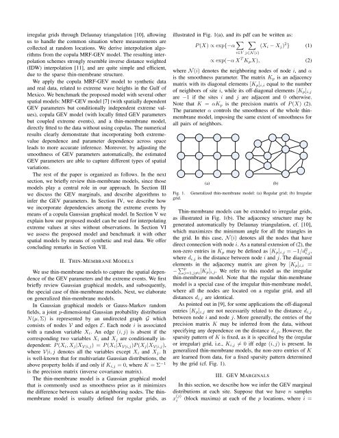
The thin-membrane model is a Gaussian graphical model
that is commonly used as smoothness prior as it minimizes
the difference between values at neighboring nodes. The thinmembrane
model is usually defined for regular grids, as
illustrated in Fig. 1(a), and its pdf can be written as:
P (X) ∝ exp{−α ∑ ∑
(X i − X j ) 2 } (1)
i∈V
j∈N (i)
∝ exp(−α X T K p X), (2)
where N (i) denotes the neighboring nodes of node i, and α
is the smoothness parameter. The matrix K p is an adjacency
matrix with its diagonal elements [K p ] i,i equal to the number
of neighbors of site i, while its off-diagonal elements [K p ] i,j
are −1 if the sites i and j are adjacent and 0 otherwise.
Note that K = αK p is the precision matrix of P (X) (2).
The parameter α controls the smoothness of the whole thinmembrane
model, imposing the same extent of smoothness for
all pairs of neighbors.
Fig. 1.
grid.
(a)
Generalized thin-membrane model: (a) Regular grid; (b) Irregular
Thin-membrane models can be extended to irregular grids,
as illustrated in Fig. 1(b). The adjacency structure may be
generated automatically by Delaunay triangulation, cf. [10],
which maximizes the minimum angle for all the triangles in
the grid. In this case, N (i) denotes all the nodes that have
direct connection with node i. As a natural extension of (2), the
non-zero entries in K p may be defined as [K p ] i,j = −1/d 2 i,j ,
where d i,j is the distance between node i and j. The diagonal
elements in the adjacency matrix are given by [K p ] i,i =
− ∑ p
j=1,j≠i [K p] i,j . We refer to this model as the irregular
thin-membrane model. Note that the regular thin-membrane
model is a special case of the irregular thin-membrane model,
where all the nodes are located on a regular grid, and all
distances d i,j are identical.
As pointed out in [9], for some applications the off-diagonal
entries [K p ] i,j are not necessarily related to the distance d i,j
between node i and node j. More generally, the entries of the
precision matrix K may be inferred from the data, without
specifying any dependence on the distance d i,j . However, the
sparsity pattern of K is fixed, as it is specified by the (regular
or irregular) grid, i.e., K i,j ≠ 0 iff edge (i, j) is present. In
generalized thin-membrane models, the non-zero entries of K
are learned from data, for a fixed sparsity pattern determined
by the grid (cf. Fig. 1).
III. GEV MARGINALS
In this section, we describe how we infer the GEV marginal
distributions at each site. Suppose that we have n samples
x (j)
i (block maxima) at each of the p locations, where i =
(b)