Dependent spatial extremes

Interestingly, the Gaussian model has the second best performance
in terms of MSE, probably due to the smooth nature
of the extreme value surface. However the KL divergence for
the Gaussian model is large compared to the other models,
since Gaussian models are not capable of capturing extreme
events; such models mostly describe fluctuations around the
mean value. Compared with the copula GEV model, the copula
MRF-GEV model achieves a smaller KL divergence with
fewer parameters, suggesting that it is beneficial to model the
spatial dependence of the GEV parameters.
We further set the scale parameter surface to be quadratic
instead of constant, as shown in Fig. 3(b). The results are
qualitatively similar. The only difference is that α σ is now
finite (4.9831), implying that the estimates of σ are no longer
independent of location. This is not surprising since the true
parameter σ follows a quadratic surface. In other words, by
inferring smoothness parameters, the smoothness of the GEV
parameters can be automatically and suitably adjusted.
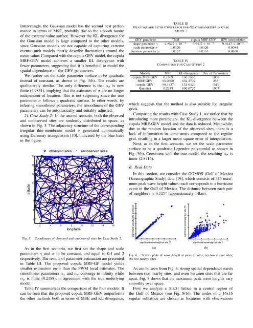
2) Case Study 2: In the second scenario, both the observed
and unobserved sites are randomly distributed in space, as
shown in Fig. 5. The adjacency structure of the corresponding
irregular thin-membrane model is generated automatically
using Delaunay triangulation [10], indicated by the blue lines
in the figure.
latitude
16
14
12
10
8
observed sites
unobserved sites
TABLE III
MEAN SQUARE ESTIMATION ERROR FOR GEV PARAMETERS IN CASE
STUDY 2
GEV parameter PWM copula MRF-GEV IDW interpolation
shape parameter γ 2.8527 × 10 −4 9.9447 × 10 −5 9.9447 × 10 −5
scale parameter σ 0.0126 0.0126 0.0084
location parameter µ 0.0157 0.0155 0.0650
TABLE IV
COMPARISON FOR CASE STUDY 2
Models MSE KL-divergence No. of Parameters
copula MRF-GEV 0.1869 150.7595 1009
MRF-GEV 95.0509 652.2792 258
copula GEV 99.1437 151.0429 1519
Gaussian 0.2283 690.6725 1007
which suggests that the method is also suitable for irregular
grids.
Comparing the results with Case Study 1, we notice that by
introducing more parameters, the KL-divergence between the
copula MRF-GEV model and the data is reduced. Meanwhile,
due to the random location of the observed sites, there is a
lack of information in some areas compared to the regular
grid, resulting in a larger mean square error of interpolation.
Next, as in the first scenario, we set the scale parameter
surface to be a quadratic Legendre polynomial as shown in
Fig. 3(b). Consistent with the true model, the resulting α σ is
finite (2.8716).
B. Real Data
In this section, we consider the GOMOS (Gulf of Mexico
Oceanographic Study) data [19], which consists of 315 maximum
peak wave height values; each corresponds to a hurricane
event in the Gulf of Mexico. The distance between each pair
of neighbors is 0.125 ◦ (approximately 14km).
6
14
15
4
2
2 4 6 8 10 12 14 16
longitude
Fig. 5. Coordinates of observed and unobserved sites for Case Study 2.
As in the first scenario, we first set the shape and scale
parameters γ and σ to be constant, and equal to 0.4 and 2
respectively. The results of parameter estimation are presented
in Table III. The proposed copula MRF-GP model yields
smaller estimation error than the PWM local estimates. The
smoothness parameters α γ and α σ converge to infinity while
α µ is finite (0.2188), in agreement with the true underlying
model.
Table IV summarizes the comparison of the four models. It
can be seen that the proposed copula MRF-GEV outperforms
the other methods both in terms of MSE and KL divergence,
significant waveheight at site 34
12
10
8
6
4
2
0
0 2 4 6 8 10 12 14
significant waveheight at site 33
(a)
significant waveheight at site 78
10
5
0
0 2 4 6 8 10 12
significant waveheight at site 1
Fig. 6. Scatter plots of wave height at pairs of sites: (a) two distant sites;
(b) two nearby sites.
As can be seen from Fig. 6, strong spatial dependence exists
between two nearby sites, and even between sites that are far
apart. Fig. 7 shows that the maximum peak wave heights vary
smoothly over space.
First we analyze a 31x31 lattice in a central region of
the Gulf of Mexico (see Fig. 8(b)). The nodes of a 16x16
regular sublattice are chosen as locations with observations
(b)