Dependent spatial extremes

where K is the precision matrix whose inverse K −1 (covariance
matrix) has normalized diagonal, Φ is the cdf of the
standard Gaussian distribution, and F i is the marginal GEV
cdf of Y i with corresponding parameters µ i , γ i and σ i . Note
that F −1
i is the pseudo-inverse of F k , which is defined as:
F −1 (x) = inf {F (y) ≥ x}. (13)
y∈Y
where y takes values in Y.
According to definition [16], a copula Gaussian graphical
model is determined by the marginals F i and the precision
matrix K. The marginals F i are GEV distributions, as described
in Section III. The spatial dependence among the GEV
marginals F i is captured by coupling the GEV parameters
through thin-membrane models (cf. Section III).
In the following, we describe how we infer the precision
matrix K. As a first step, we transform the non-Gaussian
observed variables X into Gaussian distributed latent variables
Z:
Z i = Φ −1 (F i (X i )). (14)
In the second step, for given thin-membrane sparsity structure
K p , the precision matrix K is estimated from the latent
Gaussian variables Z [17]:
ˆK = argmax log det K − trace(SK), (15)
K≻0
s.t. K i,j = 0 ∀(i, j) ∉ K p ,
where S is the empirical covariance of latent variables Z. The
convex optimization problem (15) can be solved efficiently
by the Newton-CG primal proximal point algorithm [17] or
iterative proportional fitting [18].
V. INTERPOLATION
Here we explain how extreme values can be inferred at any
location P 0 in space, including sites without observations. We
assume that the surface of the extreme values is smooth across
space. Since both spatial-dependent GEV parameters µ, γ, σ
and the latent variables Z in (11) share a (generalized) thinmembrane
structure, we will first formulate the interpolation
problem in a unified form, and then describe the minor
differences.
Let x represent the parameter vectors µ, γ, σ, or hidden
variables Z, associated to the sites with measurements, and
let x 0 denote the interpolated value at site P 0 (without measurements).
The random variables x and x 0 are assumed to
form a thin-membrane model with joint precision matrix:
( )
Kx0 K
K 0 =
x0,x
. (16)
K x,x0 K x
The conditional expected value of x 0 therefore equals:
E[x 0 |x] = −K −1
x 0
K x0,x ˆx, (17)
where ˆx is the expected value of x.
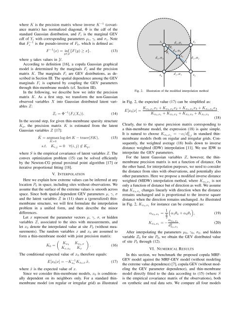
Since we consider thin-membrane models, x 0 is conditionally
dependent on its neighbors only. For a standard thinmembrane
model (on regular or irregular grid) as illustrated
Fig. 2.
x1
x2
d 4
, 4
x 4
4
1
d 1
, 1
d 0
, 0
d 3
, 3
x 0
x
d 2
, 2
Illustration of the modified interpolation method
in Fig. 2, the expected value (17) can be simplified as:
E[x 0 |x] = K x 0,x 1
x 1 + K x0,x 2
x 2 + K x0,x 3
x 3 + K x0,x 4
x 4
K x0,x 1
+ K x0,x 2
+ K x0,x 3
+ K x0,x 4
.
x 3
(18)
Clearly, due to the sparse precision matrix corresponding to
a thin-membrane model, the expression (18) is quite simple.
It is natural to choose K x0,x j
= −α/d 2 0,j in standard thinmembrane
models (both on regular and irregular grids. Consequently,
the weighted average (18) boils down to inverse
distance weighted (IDW) interpolation [11]. We use IDW to
interpolate the GEV parameters.
For the latent Gaussian variables Z, however, the thinmembrane
precision matrix is not a function of distance. On
the other hand, for interpolation purposes, we need to consider
the distance from sites with observations, and potentially also
other parameters. Here we propose a modified inverse distance
weighted (MIDW) interpolation method, where K x0,x j
is not
only a function of distance but of direction as well. We assume
that K x0,x j
changes linearly with direction when the distance
remains unchanged and is proportional to the inverse square
distance when the direction remains unchanged. As illustrated
in Fig. 2, K x0,x 1
for instance can be computed as:
α x0,x 1
= 1 )
π
(α 1 θ 4 + α 4 θ 1 , (19)
2
K x0,x 1
= − α x 0,x 1
d 2 x 0,x 1
. (20)
After interpolating the parameters µ 0 , γ 0 , σ 0 , and hidden
variable Z 0 for site P 0 , we obtain the GEV distributed value
of site P 0 through (12).
VI. NUMERICAL RESULTS
In this section, we benchmark the proposed copula MRF-
GEV model against the MRF-GEV model (without modeling
the extreme value dependence) [7], copula GEV (without modeling
the GEV parameter dependence), and thin-membrane
model directly fitted to the data according to (15) (where S
is the empirical covariance matrix of the observations), both
on synthetic and real data sets. We compare all four models