Mock-modular forms of weight one - UCLA Department of Mathematics

MOCK-MODULAR FORMS OF WEIGHT ONE 53
By Proposition 3.5, there exists mock modular forms ˜f 1 (z) ∈ M − 1 (p) and ˜f 2 (z) ∈ M + 1 (p)
with shadows f 1 , f 2 respectively such that
∑
˜f 1 (z) = c + 1 (−4)q −4 + c + 1 (−1)q −1 + c + 1 (0) +
c + 1 (n)q n ,
˜f 2 (z) = c + 2 (−2)q −2 + c + 2 (0) +
Using Proposition 3.4, we find that
∑
n>0,χ 283 (n)≠−1
n>0,χ 283 (n)≠1
c + 2 (n)q n .
−c + 1 (−4) = c + 1 (−1) = c + 2 (−2) = 2 log |u 1 u 2 2|.
Since M 1 + (p) ⊂ M + 1 (p) and M1 − (p) ⊂ M − 1 (p) are both non-empty, the principal part of ˜f j (z)
does not determine it uniquely. However, once c + 1 (2) is chosen, then ˜f 1 is fixed. Similarly,
once c + 2 (0), c + 2 (1) and c + 2 (4) are chosen, ˜f2 is fixed. Since we expect c + j (n) to be logarithms
of absolute values of algebraic numbers in F 6 , it is natural to choose c + 1 (2), c + 2 (0), c + 2 (1) and
c + 2 (4) this way and study the other coefficients. So we will write
c + j (n) = β j log |u j (n)|,
where β j ∈ Q and u j (n) ∈ C × is some complex number. Then we fix ˜f j (z) by letting
β 1 = 2, β 2 = u 2 (0) = u 2 (1) = 1 and
u 2 (4) = u 2 1(2) = − 7 16 t5 + 5 4 t4 − 7 8 t3 + 47
16 t2 − 13
16 t + 19
8 .
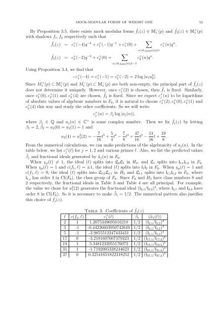
From the numerical calculations, we can make predictions of the algebraicity of u j (n). In the
table below, we list c + j (l) for j = 1, 2 and various primes l. Also, we list the predicted values
˜β j and fractional ideals generated by ũ j (n) in F 6 .
When χ p (l) ≠ 1, the ideal (l) splits into L 0 L 1 in H 3 , and L 1 splits into l l,1 l l,2 in F 6 .
When χ p (l) = 1 and c(f 1 , l) = ±1, the ideal (l) splits into l 1 l 2 in F 6 . When χ p (l) = 1 and
c(f 1 , l) = 0, the ideal (l) splits into L l,0 L l,1 in H 3 and L l,1 splits into l l,1 l l,2 in F 6 , where
l l,j has order 4 in Cl(F 6 ), the class group of F 6 . Since F 6 and H 3 have class numbers 8 and
2 respectively, the fractional ideals in Table 3 and Table 4 are all principal. For example,
the value we chose for u 2 1(2) generates the fractional ideal (l 2,1 /l 2,2 ) 4 , where l 2,1 and l 2,2 have
order 8 in Cl(F 6 ). So it is necessary to make ˜β 1 = 1/2. The numerical pattern also justifies
this choice of ˜f j (z).
Table 3. Coefficients of ˜f 1 (z)
l c(f 2 , l) c + 1 (l) ˜β1 (ũ 1 (l))
2 1 1.2075349695016218 1/2 (l 2,1 /l 2,2 ) 4
3 -1 -0.44226603950742649 1/2 (l 3,1 /l 3,2 ) 4
5 -1 -3.9855512247433431 1/2 (l 5,1 /l 5,2 ) 4
17 0 -3.2181607607379323 1/2 (l 17,1 /l 17,2 ) 4
19 1 5.3481233955176073 1/2 (l 19,1 /l 19,2 ) 4
31 1 -1.7192005338244623 1/2 (l 31,1 /l 31,2 ) 4
37 0 0.32541651822318252 1/2 (l 37,1 /l 37,2 ) 4