AE 401-- Procedure -- Lab: Nozzle Performance - Clarkson University
AE 401-- Procedure -- Lab: Nozzle Performance - Clarkson University
AE 401-- Procedure -- Lab: Nozzle Performance - Clarkson University

Create successful ePaper yourself
Turn your PDF publications into a flip-book with our unique Google optimized e-Paper software.
<strong>AE</strong> <strong>401</strong> – Spring 2005<br />
Compressible Flows and <strong>Nozzle</strong> <strong>Performance</strong><br />
J. A. Taylor ∗<br />
Mech. & Aero. Eng. Dept.<br />
<strong>Clarkson</strong> <strong>University</strong> Box 5725<br />
Potsdam, NY 13699-5725<br />
January 5, 2005<br />
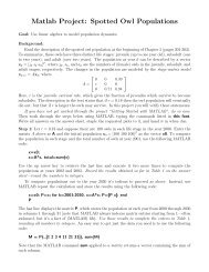
Purpose:<br />
This experiment is intended to support the Propulsion<br />
Systems and Intermediate Fluid Dynamics<br />
courses. The student will investigate the behavior<br />
of converging and converging – diverging nozzles<br />
with sufficient pressure ratios to produce transonic<br />
exit flow velocities. The student will perform measurements<br />
of the mass flow rate and the thrust and<br />
compare his or her measurements to the trends predicted<br />
using their knowledge of isentropic flows.<br />
Background:<br />
This experiment deals with the flow of a compressible<br />
fluid through nozzles. A nozzle is a suitably<br />
shaped passage in which a fluid is accelerated to<br />
a high velocity while its static pressure decreases.<br />
They are frequently used as thrust-producers for<br />
jet and rocket engines. The discussion below will<br />
provide a brief overview of compressible flows. For<br />
detailed derivations of the equations shown below,<br />
the reader is referred to: White, Frank M., Fluid<br />
Mechanics, 2nd edition, 1986, McGraw-Hill, Chap.<br />
9.<br />
Compressible fluids can not be analyzed in the<br />
same manner as incompressible flows. As a compressible<br />
flow passes through devices such as nozzles<br />
its temperature, T , pressure, P , and density, ρ,<br />
are all free to vary. Variations in these fields provides<br />
additional unknowns that must be accounted<br />
for. An additional two equations must be used to<br />
describe the flow. To simplify the analysis of the<br />
flows in this experiment, the nozzles will be modeled<br />
according to isentropic theory.<br />
Isentropic theory assumes that the entropy of<br />
the fluid remains constant throughout the nozzle.<br />
Hence, the temperature of the fluid should not<br />
change appreciably from one side of the nozzle to<br />
the other. It also predicts that a nozzle can be used<br />
both to increase the velocity of a compressible flow<br />
∗ taylorja@clarkson.edu, (315) 268-6683, and CAMP 266<br />
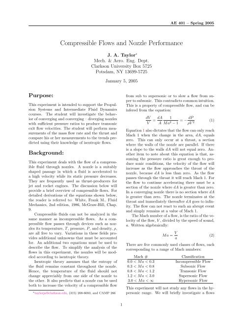
from sub to supersonic or to slow a flow from super<br />
to subsonic. This contradicts common intuition.<br />
This is a property of compressible flow, and can be<br />
infered from the equation:<br />
dV<br />
V<br />
= dA A<br />
1<br />
Ma 2 − 1 = − dP<br />
ρV 2 (1)<br />
Equation 1 also dictates that the flow can only reach<br />
Mach 1 when the change in the area, dA, equals<br />
zero. This can only occur at a throat, a section<br />
where the walls of the nozzle are parallel. If there<br />
is a slope to the walls dA will not equal zero. Another<br />
item to note about this equation is that, assuming<br />
the pressure ratio is great enough to produce<br />
sonic conditions, the velocity of the flow will<br />
increase as the flow approaches the throat of the<br />
nozzle, because dA is less than zero. As the flow<br />
passes through the throat it will reach Mach 1. For<br />
the flow to continue accelerating there must be a<br />
section of the nozzle where dA is greater than zero.<br />
In a converging nozzle there is no section where dA<br />
is greater than zero. The nozzle terminates at the<br />
throat and immediately thereafter dA goes to infinity.<br />
The flow can not react to such an abrupt event<br />
and simply remains at a value of Mach 1.<br />
The Mach number of a flow, is the ratio of the velocity<br />
of the flow, V , divided by the speed of sound,<br />
a. Written algebraically:<br />
Ma = V a<br />
(2)<br />
There are five commonly used classes of flows, each<br />
corresponding to a range of Mach numbers:<br />
Mach #<br />
Classification<br />
0.0 < Ma < 0.3 Incompressible Flow<br />
0.3 < Ma < 0.8 Subsonic Flow<br />
0.8 < Ma < 1.2 Transonic Flow<br />
1.2 < Ma < 3.0 Supersonic Flow<br />
3.0 < Ma < ∞ Hypersonic Flow<br />
This experiment will not study any flows in the hypersonic<br />
range. We will briefly investigate a flows<br />
1
<strong>AE</strong> <strong>401</strong> – Spring 2005<br />
in the hypersonic range in the shock structures experiment<br />
later in the semester. The speed of sound,<br />
a, can be calculated using the formula:<br />
a = (γRT ) 1 2<br />
(3)<br />
In Equation 3, γ is equal to the specific heat of the<br />
fluid at constant pressure divided by the specific<br />
heat at a constant volume:<br />
γ = C P<br />
C V<br />
. (4)<br />
For the air flows near STP, we will assume a value<br />
of 1.4 for γ and 287 m 2 /(s 2 k) for R. Using these<br />
assumptions, the speed of sound becomes a function<br />
of only temperature.<br />
The perfect gas law can be used to obtain the<br />
air density, rho, in the calculations for these nozzles.<br />
The perfect gas law can be written as:<br />
ρ =<br />
P RT<br />
(5)<br />
It will become important in calculations to determine<br />
the density of the air entering the nozzle,<br />
which is commonly referred to as the stagnation<br />
density, ρ o . By simply substituting the stagnation<br />
values, P o (the inlet pressure) and T o , into Equation<br />
5, the stagnation density can be determined.<br />
The following equations can be used for calculations<br />
involving the flow of air through the nozzles<br />
in this experiment:<br />
T o<br />
T = 1 + 0.2Ma2 (6)<br />
ρ o<br />
ρ = (1 + 0.2Ma2 ) 2.5 (7)<br />
P o<br />
P = (1 + 0.2Ma2 ) 3.5 (8)<br />
Rearranging these equations, we can obtain the a<br />
series of equations which can be used to obtain the<br />
Mach number:<br />
Ma 2 = 5( T o<br />
T − 1) = 5[( ρ 2<br />
o<br />
rho ) 5<br />
− 1] = 5[( P 2<br />
o<br />
P ) 7<br />
− 1]<br />
(9)<br />
From these equations the mass flow rate, ṁ, from<br />
a nozzle can be calculated. The equation for mass<br />
flow rate is:<br />
ṁ = ρA t Ma · a (10)<br />
The area, A t , and all the values of Equation 10 are<br />
evaluated at the throat of the nozzle.<br />
The mass flow rate, ṁ, will continue to increase<br />
through a nozzle until a sonic velocity is reached<br />
at the throat. When the flow through the nozzle<br />
reaches a velocity of Mach 1, the mass flow rate<br />
becomes choked. This can be explained by equation<br />
14. When the nozzle becomes choked, there is no<br />
way to increase the mass flow without increasing the<br />
throat diameter.<br />
The maximum mass flow rate, ṁ max , at γ = 1.4<br />
can be computed from the following relation:<br />
ṁ max = 0.6847P oA ∗<br />
(RT o ) 1/2 (11)<br />
The design point for a nozzle is the point at<br />
which the back pressure, P 2 , is equal to the exit<br />
pressure, P e . When a nozzle is operated that this<br />
point, it will be most efficient. If the back pressure<br />
is less than the exit pressure, the mass flow could<br />
be increased by increasing the back pressure. If the<br />
back pressure exceeds the exit pressure, the flow will<br />
be choked. The design point can be calculated for a<br />
particular nozzle with a known stagnation pressure,<br />
P o , stagnation temperature, T o , and the ratio of the<br />
throat area to the exit area, A e /A t , of the nozzle.<br />
To compute the design point of the nozzle, the<br />
exit plane Mach number, Ma e , will be needed. For<br />
dry air with γ = 1.4, an iterative approach can be<br />
used to determine the exit plane Mach number from<br />
Equation 12:<br />
A<br />
A ∗ = 1 (1 + 0.2Ma 2 ) 3<br />
Ma 1.728<br />
(12)<br />
Rather than performing the iteration over and over<br />
again, scientists have performed a series of curve fits<br />
to that directly relate the area ratio to the Mach<br />
number. For nozzles with an area ratio where 1.0 <<br />
A<br />
A ∗<br />
< 2.9 the appropriate curve fit is:<br />
Ma ≈ 1 + 1.2( A<br />
A ∗ − 1) 1/2<br />
. (13)<br />
For nozzles where the area ratio is 2.9 < A A<br />
< ∞<br />
∗<br />
the curve fit is described by:<br />
[<br />
Ma ≈ 216 A ( A<br />
) 2/3 ] 1/5.<br />
A ∗ − 254 (14)<br />
A ∗<br />
Once the exit plane Mach number is computed, the<br />
pressure ratio and the mass flow rate corresponding<br />
to the design point can be determined from equations<br />
8 and 11.<br />
A primary objective of this experiment is to<br />
show how static thrust varies with back pressure.<br />
To make any comparisons to the data obtained in<br />
the lab, we must first develop an equation to model<br />
the thrust. This equation is related to the momentum<br />
equation, and can be written as:<br />
F = ṁMa e · a + (P 1 − P 2 )A e (15)<br />
From this equation we see that the thrust, F , produced<br />
by a nozzle is a function of the mass flow<br />
rate, ṁ, the flow velocity, Ma · a, and the pressure<br />
difference, P 1 − P 2 , multiplied by the exit area, A e ,<br />
of the nozzle.<br />
2
Experiment Apparatus:<br />
These tests will be conducted using the Hilton F790<br />
<strong>Nozzle</strong> <strong>Performance</strong> Test Unit, which is located in<br />
the undergraduate lab. This apparatus, see Figure<br />
2, is essentially a fluid flow loop with suitable instrumentation<br />
for measurement of the mass flow rate,<br />
ṁ, static thrust, F , and the exit velocity of the air<br />
being discharged from a nozzle. The rig includes a<br />
regulator and an inlet control valve to control the<br />
total pressure, P 1 , upstream of the nozzle, and a<br />
chamber pressure valve to control the back pressure<br />
in the manner to which the nozzle discharges.<br />
By suitable adjustments of the latter, it is possible<br />
to set the back pressure, P 2 , to any value in the<br />
range P a ≤ P 2 ≤ P 1 , where P a is the atmospheric<br />
pressure. There are 5 interchangeable nozzles, see<br />
Figure 1, supplied with the F790 unit, all of which<br />
are axisymmetric with a minimum (or “throat”) diameter<br />
of d = 2.02mm. You will be testing nozzle<br />
no. 1 and nozzle no. 3. The first is a converging<br />
nozzle and the second is a converging-diverging nozzle<br />
with an exit area/throat area = 1.4. Each one<br />
is identified with a number stamped on its outside<br />
cylindrical surface.<br />
Stated specifically, the objectives of this experiment<br />
will be to determine the effect of backpressure<br />
P 2 upon the mass flow rate and the static thrust.<br />
This will be done for both nozzles at constant P 1 .<br />
To set up the unit for the measurements of nozzle<br />
fluid and thrust. Please proceed as follows:<br />
1. Close the air inlet valve and make sure the rig<br />
is not pressurized.<br />
2. Fully lower the contacts by rotating the micrometer<br />
screw.<br />
3. Unscrew the nuts securing the flange at the lefthand<br />
end of the chamber and withdraw the cantilever.<br />
4. Unscrew the impact head from the cantilever<br />
if it is attached, and fit the knurled nozzle<br />
adapter in its place. Make sure that the<br />
o-ring at the base of the nozzle threads<br />
is in place.<br />
5. Screw nozzle no. 1 into the adapter.<br />
6. Reassemble cantilever into chamber. Make<br />
sure that the o-ring on the flange is in<br />
place.<br />
7. Zero the micrometer dial so that for zero thrust<br />
(i.e. no flow through the nozzle) you obtain a<br />
zero dial reading. To do this, switch on the contact<br />
circuit, then rotate the micrometer screw<br />
until contact is just made. This is indicated by<br />
<strong>AE</strong> <strong>401</strong> – Spring 2005<br />
the voltmeter and lamp. The greatest sensitivity<br />
is achieved when the micrometer is adjusted<br />
until the voltmeter indicates approximately 0.5<br />
V<br />
8. The indicating dial may now be set to zero by<br />
loosening the clamping screw and rotating the<br />
dial on its spindle.<br />
9. Recheck the zero setting it should be repeatable<br />
within 0.5 of a division on the dial. If not,<br />
clean the contacts.<br />
10. Use the deflector to plug the hole in the right<br />
hand end of the chamber. Secure it with the<br />
knurled nut.<br />
11. Turn the diverter valve to the left<br />
The unit is now ready for the actual measurements<br />
of fluid and thrust. The following procedures<br />
should be followed:<br />
1. Adjust the air inlet valve and regulator to give<br />
a constant P 1 of between 500 and 900 kN/m2<br />
gage, with the chamber pressure control valve<br />
fully opened.<br />
2. Record the pressures P 1 and P 2 , the inlet temperature,<br />
T 1 , the chamber temperature, and<br />
the mass flow rate indicated by the rotameter.<br />
3. Rotate the micrometer adjustment until contact<br />
is made and the voltmeter reads 0.5V. Note<br />
the corresponding micrometer dial reading.<br />
4. Increase P 2 by about 80 kN/m 2 and repeat<br />
steps 2 and 3. Make sure you keep P 1 constant<br />
throughout.<br />
5. Take readings for each such P 2 until you finally<br />
reach P 2 = P 1 .<br />
When you reach step 5 you have finished taking<br />
data for nozzle no.1. Now close the inlet valve and<br />
open the chamber valve. When the chamber has<br />
been fully is discharged, replace nozzle no. 1 by<br />
nozzle no. 3. Take the same set of measurements<br />
(as per steps 1-5 above) for nozzle no. 3, making<br />
sure you use the same P 1 .<br />
# Type A exit /A throat P exit /P inlet<br />
1 Convergent 1.0 1.0 – 0.528<br />
2 Conv. – Div. 1.2 0.260<br />
3 Conv. – Div. 1.4 0.185<br />
4 Conv. – Div. 1.6 0.140<br />
5 Conv. – Div. 2.0 0.095<br />
Table 1: <strong>Nozzle</strong> geometries<br />
3
<strong>AE</strong> <strong>401</strong> – Spring 2005<br />
1 2 3 4 5<br />
;; ;;<br />
;; ;;<br />
;; ;;<br />
;; ;;<br />
;; ;;<br />
;; ;;<br />
;; ;;<br />
2.0mm<br />
;;<br />
;;<br />
;;<br />
;;<br />
;;<br />
;;<br />
;;<br />
;;<br />
;;<br />
;;<br />
;;<br />
;;<br />
;;<br />
;;<br />
;;<br />
;;<br />
;;<br />
;;<br />
;;<br />
;;<br />
;;<br />
;;<br />
;;<br />
;;<br />
;;<br />
;;<br />
;;<br />
;<br />
;<br />
;<br />
;<br />
;<br />
;<br />
;<br />
;<br />
;<br />
;<br />
;<br />
;<br />
;;<br />
;;<br />
;;<br />
;;<br />
;;<br />
;;<br />
;;<br />
;;<br />
;;<br />
;;<br />
;;<br />
10 O<br />
Thrust Force [ N ]<br />
4.5<br />
4<br />
3.5<br />
3<br />
2.5<br />
2<br />
1.5<br />
1<br />
0.5<br />
0<br />
Calibration Data<br />
y = 0.044185x - 0.033807<br />
-0.5<br />
0 10 20 30 40 50 60 70 80 90 100<br />
Micrometer Reading<br />
Figure 1: <strong>Nozzle</strong> Geometries<br />
Figure 3: Micrometer calibration curve.<br />
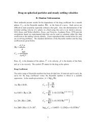
A rotameter is used to measure the mass flow<br />
rate, ṁ, through the nozzle. The scale on the rotameter<br />
is incremented in millimeters. The calibration<br />
curve is used to convert from millimeters to the<br />
mass flow rate. The calibration curve is shown in<br />
Figure 4. Make sure you apply the density correction<br />
factor k that can be obtained from Figure 5 or<br />
Equation 17.<br />
9<br />
8<br />
Calibration Data<br />
y = 0.8895 + 0.0292x + 2.34e-5x 2<br />
7<br />
Figure 2: Apparatus for <strong>Nozzle</strong> Tests<br />
Instrumentation<br />
The thrust force is measured using what is effectively<br />
a beam type load cell. The nozzle is threaded<br />
into the end of a long section of tubing. The thrust<br />
force produced as a result of mass being thrown<br />
from the nozzle, causes the beam to deflect downward.<br />
From our strengths of materials studies, we<br />
know that a cantilever beam with concentrated load<br />
can be described as:<br />
y = F l3<br />
3EI<br />
(16)<br />
The modulus of elasticity, E, the length of the<br />
beam, l, and the moment of inertia, I, are all<br />
constant which indicates that the deflection of the<br />
beam, y should vary linearly with the thrust force,<br />
F . Figure 3 demonstrates this and provides an<br />
equation relating the displacement to thrust force.<br />
Air Flow Rate / 10 - 3 kg ⋅ s - 1<br />
6<br />
5<br />
4<br />
3<br />
2<br />
1<br />
0<br />
0 20 40 60 80 100 120 140 160 180 200 220 240<br />
Scale [ mm ]<br />
Figure 4: Calibration curve for 35E rotameter with<br />
duralumin float. Note: Curve is correct for ρ =<br />
1.2kg · m −2 . Multiply mass flow rate by correction<br />
factor, k, from Figure 5.<br />
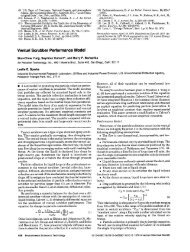
The rotameter calibration correction factor, k,<br />
can be extracted from Figure 5. To obtain a reasonable<br />
estimate of the correction factor from the plot,<br />
the atmospheric pressure, P a and ambient temperature,<br />
T , must be measured. The atmospheric pressure<br />
can be measured using the mercury barometer<br />
located on the wall near the safety goggle cabinet.<br />
4
<strong>AE</strong> <strong>401</strong> – Spring 2005<br />
With these readings, you can locate the appropriate<br />
pressure on the horizontal axis, and then you<br />
should be able to linearly interpolate between the<br />
temperature curves. Equation 17 has been provided<br />
to reduce the effort associated with determining the<br />
correction factor.<br />
Rotameter Correction Factor, k<br />
1.03<br />
1.02<br />
1.01<br />
1<br />
0.99<br />
0.98<br />
0.97<br />
10 o C - Air Temp.<br />
20 o C - Air Temp.<br />
30 o C - Air Temp.<br />
40 o C - Air Temp.<br />
0.96<br />
0.96 0.97 0.98 0.99 1 1.01 1.02 1.03 1.04<br />
Atmospheric Pressure / 100 kN ⋅ m - 2<br />
Figure 5: Correction factor, k, for 35E rotameter.<br />
( 2∑<br />
k ≈ m i T i) ( 2∑<br />
· P a + b i T i) (17)<br />
i=0<br />
i=0<br />
i m i b i<br />
0 0.52475 0.50301<br />
1 -0.00665 0.00499<br />
2 0.00015 -0.00015<br />
Tasks:<br />
Now the remainder of your job is to suitably reduce,<br />
display, and interpret the experimental data.<br />
1. Plot the measured flow rate, ṁ (gm/s) vs. the<br />
pressure ratio P 2 / P 1 , making sure that P 2 and<br />
P 1 are both expressed as absolute pressures.<br />
or your model be modified to improve the<br />
agreement?<br />
(d) Indicate on your graph the ranges of P 2 /<br />
P 1 over which the two nozzles are choked.<br />
2. Plot the measured static thrust, F , vs. the<br />
pressure ratio P 2 / P 1 .<br />
(a) Plot data from both nozzles on the same<br />
graph using the same symbols as you did<br />
on the graph of mass flow rate.<br />
(b) Plot (as a solid line) the F that is predicted<br />
by one-dimensional isentropic flow<br />
theory as a function P 2 / P 1 for nozzle no.<br />
1.<br />
(c) Does the theoretical curve agree well with<br />
your test data for nozzle no. 1? If not,<br />
why not?<br />
3. The flow in a converging-diverging nozzle is<br />
fairly complex. It may, depending upon the<br />
value of P 2 / P 1 , include normal shock waves<br />
in the diverging section or complex supersonic<br />
phenomena which occurs beyond its exit plane.<br />
In his text, White indicates that it is desirable<br />
to operate near the so-called design point of the<br />
nozzle. Calculate the exit plane Mach number,<br />
Ma, and the static thrust, F , at the design<br />
point and compare it the value of F that was<br />
measured.<br />
References:<br />
White, F.M., (1979), Fluid Mechanics, 2 n d Edition,<br />
McGraw-Hill, Inc., New York, New York, USA,<br />
Chapter 9<br />
(a) Plot the data you measured for both nozzles<br />
on the same graph, identifying the<br />
data points for nozzle no. 1 with one symbol<br />
and those for nozzle no. 3 with another<br />
symbol. Use errorbars to indicate<br />
the uncertainty in your measurements.<br />
(b) Plot (as a solid line) the theoretical curve<br />
of ṁ vs. P 2 / P 1 for a converging nozzle<br />
(like nozzle no.1) which may be predicted<br />
assuming one-dimensional isentropic flow.<br />
(c) Does the theoretical curve agree well with<br />
your test data for nozzle no. 1? If not,<br />
why not and how could the experiment<br />
5