Overview of Capital Account Crisis - IMF

- 11 -
could not reduce their exposure to the government to meet the deposit outflow without
triggering a government funding crisis, and instead had to run down their own external
assets—the one asset that would have continued to perform in the event of default and
devaluation. Banks also had to reduce their domestic currency lending to the private
sector, though these were more likely to perform in the event of a devaluation.
Crisis trigger
17. Argentina’s experience illustrates how currency and maturity mismatches in the
public and private sector balance sheets can interact to exacerbate vulnerabilities. But what
triggered the crisis? In contrast to some other capital account crises (e.g., Uruguay) where a
specific event triggered the crisis, Argentina’s 2002 crisis was the culmination of a prolonged
period over which it became increasingly apparent that fiscal policy was not consistent with
the pegged exchange rate under the currency board arrangement regime. Traditional currency
crisis models would suggest that if the central bank expands domestic credit at a faster rate
then the growth in money demand, then the exchange rate peg will eventually collapse.
However, this was not the case in Argentina, where the central bank largely remained within
the strictures of the currency board regime. Nevertheless, Argentina’s fiscal policy was
intertemporally inconsistent with its exchange rate peg.
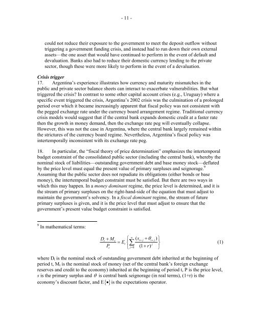
18. In particular, the “fiscal theory of price determination” emphasizes the intertemporal
budget constraint of the consolidated public sector (including the central bank), whereby the
nominal stock of liabilities—outstanding government debt and base money stock—deflated
by the price level must equal the present value of primary surpluses and seignorage. 9
Assuming that the public sector does not repudiate its obligations (either bonds or base
money), the intertemporal budget constraint must be satisfied. But there are two ways in
which this may happen. In a money dominant regime, the price level is determined, and it is
the stream of primary surpluses on the right-hand-side of the equation that must adjust to
maintain the government’s solvency. In a fiscal dominant regime, the stream of future
primary surpluses is given, and it is the price level that must adjust to ensure that the
government’s present value budget constraint is satisfied.
9 In mathematical terms:
∞
D ( )
t
+ M ⎧ s
t
t+ j
+ θt+
j ⎫
= E
t ⎨∑ j ⎬
(1)
Pt
⎩ j=
0 (1 + r)
⎭
where D t is the nominal stock of outstanding government debt inherited at the beginning of
period t, M t is the nominal stock of money (net of the central bank’s foreign exchange
reserves and credit to the economy) inherited at the beginning of period t, P is the price level,
s is the primary surplus and θ is central bank seignorage (in real terms), (1+r) is the
economy’s discount factor, and E{ •}
is the expectations operator.