Code Space Dimension of Translation-Invariant Qubit Stabilizer Codes
Code Space Dimension of Translation-Invariant Qubit Stabilizer Codes
Code Space Dimension of Translation-Invariant Qubit Stabilizer Codes

Create successful ePaper yourself
Turn your PDF publications into a flip-book with our unique Google optimized e-Paper software.
<strong>Code</strong> <strong>Space</strong> <strong>Dimension</strong> <strong>of</strong><br />
<strong>Translation</strong>-<strong>Invariant</strong> <strong>Qubit</strong> <strong>Stabilizer</strong> <strong>Code</strong>s<br />
von<br />
Andrés Wilhelm Goens Jokisch<br />
Bachelorarbeit in Physik<br />
vorgelegt der<br />
Fakultät für Mathematik, Informatik und<br />
Naturwissenschaften der RWTH Aachen<br />
im November 2011<br />
angefertigt im<br />
Institut für Quanteninformation bei<br />
Pr<strong>of</strong>. Dr. Barbara M. Terhal
Ich versichere, dass ich die Arbeit selbstständig verfasst und keine anderen<br />
als die angegebenen Quellen und Hilfsmittel benutzt, sowie Zitate kenntlich<br />
gemacht habe.<br />
Aachen, den 4. November 2011<br />
2
Contents<br />
0.1 A Note on Notation . . . . . . . . . . . . . . . . . . . . . . . . 4<br />
1 Introduction 5<br />
2 <strong>Qubit</strong>s and <strong>Stabilizer</strong> <strong>Code</strong>s 6<br />
2.1 Classical <strong>Code</strong>s . . . . . . . . . . . . . . . . . . . . . . . . . . 6<br />
2.1.1 Linear <strong>Code</strong>s . . . . . . . . . . . . . . . . . . . . . . . 6<br />
2.1.2 Dual <strong>Code</strong>s . . . . . . . . . . . . . . . . . . . . . . . . 7<br />
2.1.3 <strong>Code</strong> Distance . . . . . . . . . . . . . . . . . . . . . . . 8<br />
2.2 <strong>Qubit</strong>s and quantum codes . . . . . . . . . . . . . . . . . . . . 8<br />
2.3 Error correction . . . . . . . . . . . . . . . . . . . . . . . . . . 9<br />
2.4 The stabilizer formalism . . . . . . . . . . . . . . . . . . . . . 12<br />
2.5 Logical Operators . . . . . . . . . . . . . . . . . . . . . . . . . 14<br />
2.6 <strong>Code</strong> distance . . . . . . . . . . . . . . . . . . . . . . . . . . 16<br />
2.7 CSS <strong>Code</strong>s . . . . . . . . . . . . . . . . . . . . . . . . . . . . . 17<br />
3 Geometrical Quantum <strong>Code</strong>s 18<br />
3.1 The Surface <strong>Code</strong> . . . . . . . . . . . . . . . . . . . . . . . . 18<br />
3.2 Self-correcting Quantum Memory . . . . . . . . . . . . . . . . 21<br />
3.3 The STS model . . . . . . . . . . . . . . . . . . . . . . . . . . 22<br />
3.4 A Classic Self-Correcting Memory And The Energy Barrier . 23<br />
3.5 The Haah <strong>Code</strong> . . . . . . . . . . . . . . . . . . . . . . . . . . 24<br />
4 <strong>Translation</strong>-<strong>Invariant</strong> <strong>Stabilizer</strong> <strong>Code</strong>s 25<br />
4.1 <strong>Stabilizer</strong> codes on a lattice with periodic boundary conditions 25<br />
4.2 <strong>Translation</strong>-invariant codes on lattices as factor rings <strong>of</strong> polynomial<br />
rings . . . . . . . . . . . . . . . . . . . . . . . . . . . . 29<br />
4.3 The dimension <strong>of</strong> factor rings <strong>of</strong> polynomial rings . . . . . . . 37<br />
5 Conclusion 41<br />
A Mathematical Supplement 42<br />
3
0.1 A Note on Notation<br />
This thesis uses many concepts from abstract algebra. Appendix A has a<br />
supplement on many terms, and can be consulted when in doubt about a<br />
specific definition. The following list is a small reference on a few notational<br />
conventions used on the thesis:<br />
• n := {1, 2, . . . , n}<br />
• < ⃗e 1 , ⃗e 2 > Z := {x⃗e 1 + y⃗e 2 | x, y ∈ Z}<br />
• A ⊳ B means that A is an ideal or normal subgroup <strong>of</strong> B, depending on<br />
the context (if B is a ring or a just a group)<br />
• f | g means that f divides g, i.e. ∃h : g = fh.<br />
• f ∤ g means that f does not divide g.<br />
• < g 1 , . . . , g n >:= {h 1 · · · h k | h i ∈ {g 1 , g −1<br />
1 , g 2 , g −1<br />
2 , . . . , g n , g −1<br />
n } ∀ i ∈ k}<br />
the group generated by g 1 , . . . , g n .<br />
• F 2 = GF(2) The finite field, or galois field, with two elements.<br />
4
1 Introduction<br />
Quantum information and quantum computation are fields <strong>of</strong> much interest,<br />
not only from a theoretical standpoint, but also quite practically for<br />
building a quantum computer. Classical computers are not perfect: during<br />
the storage, transmission and processing they are bound to make errors and<br />
corrupt the data. There is a mature theory in mathematics which helps<br />
deal with that: coding theory. Through coding theory we can reliably store,<br />
transmit and process data in classical computers, but what about quantum<br />
computers? Through quantum codes, an analogous concept to what is used<br />
in classical computers, we try to do the same for quantum computers. In<br />
this thesis we will briefly introduce both, classical and quantum codes and<br />
we will develop a very important class <strong>of</strong> quantum codes called stabilizer or<br />
additive codes.<br />
With the idea <strong>of</strong> application in mind, we will investigate a subclass stabilizer<br />
codes: geometrical stabilizer codes. It has the advantage <strong>of</strong> being a<br />
physically plausible model. We will introduce the concept <strong>of</strong> a self-correcting<br />
quantum memory, and look for codes which could realize one in this subclass.<br />
We will study STS codes, a subclass <strong>of</strong> geometrical stabilizer codes, which<br />
amongst others, has a code space dimension that is independent <strong>of</strong> the lattice<br />
size. We will see that it was proven by Yoshida in [9] that STS codes are not<br />
to be feasible for self-correcting quantum memory. After this, we will study<br />
a code proposed by Haah in [3] which escapes this conclusion, and motivated<br />
by this code, we will develop a formalism for a larger class <strong>of</strong> codes without<br />
the assumption on the code space dimension. Using this formalism we will<br />
develop an algorithm for calculating this dimension and apply it to Haah’s<br />
code.<br />
Acknowledgements:<br />
First and foremost, I would like to thank Barbara Terhal for her feedback,<br />
for her help with the subject and especially for her patience with me while<br />
writing this thesis. I would also like to thank Jeongwan Haah for sharing his<br />
unpublished notes which were a central to the main part <strong>of</strong> this thesis. Last,<br />
I would like to thank my parents; in particular my mother, for helping me<br />
with the pro<strong>of</strong>-reading for the language used in here.<br />
5
2 <strong>Qubit</strong>s and <strong>Stabilizer</strong> <strong>Code</strong>s<br />
2.1 Classical <strong>Code</strong>s<br />
Before we study quantum codes, it might be a good idea to get at least a<br />
very small feel for classical error-correcting codes. Classical error-correcting<br />
codes are a mathematical structure that we experience every day. They are<br />
mainly used to make sure a message arrives, even through a channel that<br />
can produce errors. Speech itself is a rather complex code: we can usually<br />
understand someone, even when there is some background noise, or when<br />
the person speaking makes a small mistake. Much staighter forward are for<br />
instance the codes used on CD-roms, which are called linear codes (Reed-<br />
Solomon codes are a specific example used on CD-ROMs). Linear codes will<br />
only be briefly introduced to give an idea <strong>of</strong> coding theory.<br />
2.1.1 Linear <strong>Code</strong>s<br />
Before we get into a mathematical definition <strong>of</strong> linear codes, it might be<br />
prudent to refresh a few simple concepts.<br />
F 2 (sometimes also called GF(2)) is a field, just like R or C, in which<br />
there is an addition + and a multiplication ·, but has only two elements. We<br />
shall call these 0 and 1 respectively. To calculate in F 2 , we can calculate over<br />
R and take the result modulo 2. By the way, this would work for any prime<br />
number instead <strong>of</strong> 2, yielding other finite fields, but we are not interested in<br />
them here. Concepts like vector spaces, subspaces and dimension work for<br />
F 2 , just as they do for R or C.<br />
Definition 2.1. A linear code C coding k bits on n bits, also called [n,k]-<br />
<strong>Code</strong> is a k-dimensional F 2 subspace <strong>of</strong> F n 2.<br />
The problem <strong>of</strong> saving the code in some way (knowing what the codewords<br />
are) and <strong>of</strong> encoding some message, is easily solved by using so-called<br />
generator matrices. If you take a basis b 1 , . . . , b k <strong>of</strong> the code C as a subspace<br />
<strong>of</strong> F n 2, and let G be the matrix with b 1 , . . . , b k as columns, then you get the<br />
code as the span <strong>of</strong> this matrix G. Even further, if v ∈ F k 2 is some k-bit<br />
string, coded as a column vector, then you can encode v just by calculating<br />
Gv ∈ F n 2, which is read as an n-bit string. Note that the generator matrix is<br />
not unique, and so the encoding might differ. This must be kept in mind for<br />
decoding.<br />
Example 2.2. One <strong>of</strong> the simplest linear codes there are, is the repetition<br />
code. You just repeat the bit three times: you code 0 as 000, and 1 as 111. If<br />
later an error occurs and you get the string 101, it is more likely that it was<br />
6
a 111 than a 000, that is assuming only one error can occur, we can retrieve<br />
the original bit. We say that this code corrects one error. A basis for this<br />
code is b 1 = (1, 1, 1) T , where v T denotes the transpose.<br />
⎡<br />
then G = ⎣<br />
1<br />
1<br />
1<br />
⎤<br />
⎦ is a Generator matrix for the repetition code.<br />
Another important concept is that <strong>of</strong> the parity-check matrix, which tends<br />
to be more useful for error correction. Instead <strong>of</strong> a generating set, we let H be<br />
a matrix with kernel C, that is with Hv = 0 iff v ∈ C. It is straightforward<br />
to get the parity-check matrix from the code, but we will not dwell into that.<br />
What this means is that we can easily detect if a received message is<br />
part <strong>of</strong> the code, in which case we assume it was sent correctly. While<br />
strictly speaking it might not be the case, we assume some maximal number<br />
<strong>of</strong> mistakes which would rule it out. If while sending the coded message<br />
m ∈ F n 2 some minor error e ∈ F n 2 happened, where e has a 1 in each place<br />
where an error has occurred, then by applying the parity check matrix H we<br />
get the so-called syndrome: s = H(m + e). Here, the linearity <strong>of</strong> the code<br />
(for it being represented by matrices) comes into play:<br />
s = H(m + e) = Hm + He = 0 + He<br />
So the syndrome is directly related to the error. From here we can proceed,<br />
using the syndrome s, to find e and correct the code. We will not get into<br />
the specifics <strong>of</strong> this.<br />
Example 2.3. For the repetition code above, a parity-check matrix is given<br />
by<br />
[ ] 1 1 0<br />
H =<br />
0 1 1<br />
2.1.2 Dual <strong>Code</strong>s<br />
The main advantage <strong>of</strong> linear codes is that they have an algebraic structure<br />
which can be used in many ways. One <strong>of</strong> these is by defining a bilinear form<br />
on the code:<br />
Definition 2.4. Let b = (b 1 , . . . , b n ), c = (c 1 , . . . , c n ) ∈ F n 2 be two codewords.<br />
Define < b, c >:= ∑ n<br />
i=1 b ic i ∈ F 2 to be the product <strong>of</strong> b and c. < ·, · > thus<br />
defines what is called a symmetric bilinear form, which is a generalization <strong>of</strong><br />
the scalar product in a sense.<br />
7
Bilinear forms are an object that has been studied intensively in mathematics.<br />
One thing we immediately get from introducing this product is the<br />
concept <strong>of</strong> duality, and in particular, <strong>of</strong> basis independent dual space to the<br />
code space.<br />
Definition 2.5. Let C ≤ F n 2 be a linear code. Set C ⊥ := {v ∈ F n 2 |< v, c >=<br />
0 ∀ c ∈ C}. C ⊥ is called the dual code to C. From the theory <strong>of</strong> bilinear<br />
forms we immediately get the result: Dim C + Dim C ⊥ = n, so we know<br />
directly what the number <strong>of</strong> encoded bits is. A code which satisfies C ⊆ C ⊥<br />
is called weakly self dual, and self dual if C = C ⊥ . Note that this means<br />
that for a self dual code, n has to be even and Dim C = n 2 .<br />
2.1.3 <strong>Code</strong> Distance<br />
One last important concept from classical coding theory, which has an important<br />
analogous concept in quantum codes, is the distance <strong>of</strong> a code. First,<br />
we have to introduce some sort <strong>of</strong> measure <strong>of</strong> distance in the code.<br />
Definition 2.6. Let C ≤ F n 2 be a linear code, and c (1) , c (2) ∈ C. The weight<br />
<strong>of</strong> c (1) is defined as wt(c (1) ) := |{i ∈ n | c (1)<br />
i ≠ 0}|, i.e. the number <strong>of</strong> bits <strong>of</strong><br />
c (1) that are not 0. The Hamming distance between c (1) and c (2) is defined<br />
similarly, as the number <strong>of</strong> different bits between them: d(c (1) , c (2) ) = |{i ∈<br />
n | c (1)<br />
i ≠ c (2)<br />
i }| = wt(c (1) − c (2) ). For the whole code, the minimal distance<br />
and minimal weight, which for linear codes are the same, are defined as:<br />
min c,c ′ ∈C d(c, c ′ ) = min 0≠c∈C wt(c).<br />
Probably by far the most important property <strong>of</strong> the minimal distance<br />
is that a code with distance d can always correct up to t < d errors. The<br />
2<br />
reason for this is simple to understand, since if t < d errors occur, then the<br />
2<br />
distance between the received bit string and the original codeword will be<br />
strictly smaller than the distance between the received string and any other<br />
codeword, by definition <strong>of</strong> the minimal distance.<br />
2.2 <strong>Qubit</strong>s and quantum codes<br />
The main subjects <strong>of</strong> this thesis are quantum codes. For these, we no longer<br />
work with bits, but instead do so with so-called ’qubits’, or ’quantum bits’.<br />
Definition 2.7. A qubit is a two dimensional C vector space, C 2 . It is an<br />
abstraction <strong>of</strong> a two state quantum system, whose physical realization we<br />
disregard, and is described by the Hilbert space H = C 2 . For convention we<br />
will call two orthonormal states <strong>of</strong> H |0〉 and |1〉 in analogy to the two states<br />
<strong>of</strong> a bit, 0 and 1. Hence, span(|0〉, |1〉) = H.<br />
8
Remark 2.8. A many qubit system is, as by the postulates <strong>of</strong> quantum<br />
mechanics, described by the tensor product Hilbert space <strong>of</strong> its single qubits.<br />
This is the reason why an n-qubit system is described by H = C<br />
} 2 ⊗ .<br />
{{<br />
. . ⊗ C<br />
}<br />
2 ∼ =<br />
n times<br />
C 2n . The basis <strong>of</strong> this space given by the |0〉, |1〉 basis for each qubit can be<br />
abbreviated by binary strings: |b 1 b 2 . . . b n 〉 := |b 1 〉 ⊗ |b 2 〉 . . . ⊗ |b n 〉. For instance<br />
|010〉 = |0〉 ⊗ |1〉 ⊗ |0〉. This notation also makes the analogy to bits<br />
further clear, hence the name, qubits.<br />
Just as we did with linear classical codes, we can now define quantum<br />
codes:<br />
Definition 2.9. A quantum code C is a (linear) subspace <strong>of</strong> an n-qubit space<br />
C 2n . If the code is a 2 k dimensional subspace <strong>of</strong> C 2n for some integer k ≤ n,<br />
then we call the code C an [[n, k]]-<strong>Code</strong>. In this case there is a bijective linear<br />
mapping from a k-qubit system to the code C. We say the code encodes k<br />
qubits in n qubits.<br />
We shall now see how these codes help correct errors in qubits.<br />
2.3 Error correction<br />
What good is a code if it does not correct errors? We will see with the<br />
same example from classical coding theory, the repetition code, how error<br />
correction can work in principle. Before we do so, however, we must first<br />
consider what kinds <strong>of</strong> error can happen. From the postulates <strong>of</strong> quantum<br />
mechanics we know that the time evolution <strong>of</strong> a closed system is given by<br />
a unitary operator. This means that in principle, any unitary operator can<br />
act on the code. There is, however, no reason for the system to be closed:<br />
it will interact with the environment, meaning that measurements can also<br />
be made, amongst others. There is a formalism called quantum operation<br />
formalism that describes all these errors; a development <strong>of</strong> this formalism<br />
can be found in [2]. Here we will restrict ourselves to unitary operators. We<br />
will concentrate only on a small subset <strong>of</strong> these, the so-called Pauli group,<br />
which will turn out to be enough thanks to theorem 2.13:<br />
Definition 2.10. The one-qubit unitary operators defined by<br />
[ ] [ ] [ ]<br />
0 1 0 i 1 0<br />
I, X = , Y = , Z =<br />
1 0 −i 0 0 −1<br />
(1)<br />
are called Pauli operators.<br />
9
On n qubits, the operators <strong>of</strong> the form σ 1 ⊗. . .⊗σ n , where σ i ∈ {I, X, Y, Z}<br />
for all i, are called n-qubit Pauli operators. If you take all products <strong>of</strong> n-qubit<br />
Pauli operators you get a finite group P n , called the Pauli group. It is easy<br />
to see that P n = {i j σ 1 ⊗ . . . ⊗ σ n | σ k ∈ {I, X, Y, Z} for all k ∈ n, j ∈ 4}.<br />
Example 2.11. A first, naive approach for building a quantum code is just<br />
the repetition code in qubits:<br />
|0〉 ↦→ |000〉<br />
|1〉 ↦→ |111〉<br />
It is not hard to see that this code will protect from one Pauli X error, for<br />
example, X 2 :<br />
X 2 |000〉 = |010〉<br />
And just as in the classical analog, we can see this (assuming only one X i<br />
error) can only have been |000〉. It is not difficult to see that this code will<br />
protect from a single X i error on an arbitrary qubit. Simple, right? The<br />
problem is, we have to measure in some way the state <strong>of</strong> the code in order<br />
to find out what the state is and what error happened. Fortunately, there<br />
is a way <strong>of</strong> covering all ’bit flip’ (X i ) errors with a measurement: Define the<br />
following measurement operators:<br />
P 0 := |000〉〈000| + |111〉〈111|, P 1 := |100〉〈100| + |011〉〈011|<br />
P 2 := |010〉〈010| + |101〉〈101|, P 3 := |001〉〈001| + |110〉〈110|<br />
From the operators themselves it is easy to see that a measurement in<br />
this basis will immediately identify if exactly one ’bit flip’ error (but nothing<br />
else) has happened, and leave everything as it is.<br />
This example also shows the problem mentioned at the beginning <strong>of</strong> this<br />
section; that unlike in classical coding theory, there is a continuous, infinite<br />
set <strong>of</strong> possible errors (SU(2, C) for a single qubit). Consider the state |+〉 :=<br />
1/ √ 2(|0〉 + |1〉). Coding this would yield 1/ √ 2(|000〉 + |111〉). Since all error<br />
operators are linear, a bit flip would still be corrected with the measurement<br />
above. But how about a phase flip? Consider the error Z 1 , for example.<br />
Z 1 ( √ 1<br />
2<br />
(|000〉 + |111〉)) = √ 1<br />
2<br />
(|000〉 − |111〉), which would go undetected, but<br />
would be decoded to be |−〉 := 1/ √ 2(|0〉 − |1〉).<br />
We can modify the code to detect phase flip (Z i ) errors: We have seen that<br />
the operator Z takes |+〉 to |−〉 and vice-versa. That is, it flips both states.<br />
If we were to rename our states |0〉 and |1〉, Z would act as an X. With this<br />
in mind, it is not difficult to see why coding |0〉 ↦→ | + ++〉, |1〉 ↦→ | − −−〉<br />
10
would be a good idea. If we make the same measurement as in example 2.11,<br />
but in the |+〉, |−〉 basis instead, a phase flip would be the same as a bit flip<br />
in that basis, and would be detected. It can be immediately checked that<br />
the operator<br />
H = √ 1 [ ] 1 1<br />
2 1 −1<br />
also called a Haddamard gate, takes (|0〉, |1〉) ↦→ (|+〉, |−〉). So the measurement<br />
operators would be HP i H † = HP i H, i = 0, 1, 2, 3.<br />
But this code, again, would not be able to detect a bit flip. We can try<br />
combining them, on a 9 qubit code:<br />
Example 2.12. This 9 qubit code, also known as Shor code [2] can correct<br />
an X or Z error on a single qubit. This is achieved by combining the<br />
two codes previously mentioned. First the phase flip code, |0〉 ↦→ | + ++〉,<br />
|1〉 ↦→ | − −−〉, then the bit flip code to each <strong>of</strong> the three qubits <strong>of</strong> the first<br />
encoding: | + ++〉 = |+〉|+〉|+〉 = √ 1<br />
2<br />
(|0〉 + |1〉) √ 1<br />
2<br />
(|0〉 + |1〉) √ 1<br />
2<br />
(|0〉 + |1〉) ↦→<br />
1<br />
2 √ (|000〉 + |111〉)(|000〉 + |111〉)(|000〉 + |111〉) and in an analogous fashion<br />
2<br />
| − −−〉 ↦→ 1<br />
2 √ = (|000〉 − |111〉)(|000〉 − |111〉)(|000〉 − |111〉)<br />
2<br />
This, we have seen, can correct a single one <strong>of</strong> two different errors on a<br />
single qubit. It might seem like a lot <strong>of</strong> work for very little gain. Fortunately,<br />
as we will see, the correcting <strong>of</strong> these two errors is enough to correct an<br />
arbitrary single-qubit error! In fact, the following theorem ( 2.13) is one <strong>of</strong><br />
the results that make quantum error correction possible in the first place,<br />
since it helps to bypass the problem <strong>of</strong> a continuous, infinite set <strong>of</strong> possible<br />
errors.<br />
Theorem 2.13. Let {E i | i ∈ I} for some index set I be a set <strong>of</strong> unitary<br />
operators, and C be a quantum code that can correct errors on all these<br />
E i , i ∈ I. Further let {F j | j ∈ J} for another index set J be another<br />
set <strong>of</strong> unitary operators, which is a linear combination <strong>of</strong> the E i , i.e. F j =<br />
∑<br />
i∈I c i,jE i for all j ∈ J and for some c i,j ∈ C. Then, C can also correct<br />
all errors F j , j ∈ J. This theorem actually holds for a wider class <strong>of</strong> errors,<br />
where E i , F j are quantum operations; but this goes beyond the scope <strong>of</strong> this<br />
thesis. The more general statement, along with a pro<strong>of</strong>, can be found in [2].<br />
Now, with a feel for quantum codes, we can start studying the stabilizer<br />
codes, a very important class <strong>of</strong> quantum codes with a core role for this<br />
thesis:<br />
11
2.4 The stabilizer formalism<br />
Before we get into the formalism itself, we need to cover some background.<br />
Remark 2.14. The Pauli Group P n has the following interesting properties:<br />
• Two operators in the Pauli group either commute or anti-commute, i.e.<br />
∀ A, B ∈ P n : [A, B] = AB −BA = 0 or {A, B} = AB +BA = 0. This<br />
follows immediately from its being a property <strong>of</strong> the Pauli matrices.<br />
• The commutator subgroup <strong>of</strong> the Pauli group, defined as P ′ n := {ABA −1 B −1 |<br />
A, B ∈ P n } is given by P n = {±I}, which is another way <strong>of</strong> saying that<br />
they only commute or anticommute.<br />
• The centre <strong>of</strong> the Pauli group, defined as Z(P n ) = {A ∈ P n | AB =<br />
BA for all B ∈ P n } is given by Z(P n ) = {±I, ±iI}.<br />
• The factor group P n /Z(P n ) is an n-dimensional F 2 vector space. This<br />
property is a special case <strong>of</strong> the Burnside basis theorem, see [13].<br />
• Every element in the Pauli group can be written as follows:<br />
i j X a 1<br />
1 Z b 1<br />
1 X a 2<br />
2 Z b 2<br />
2 . . . X an<br />
n Z bn<br />
n (2)<br />
where j ∈ {0, 1, 2, 3}, a i , b i ∈ {0, 1} ∀ i ∈ n . That this is true can be<br />
seen immediately from Y = iXZ and the fact that elements commute<br />
or anti-commute.<br />
A more detailed analysis <strong>of</strong> the Pauli group can be found in [5]. There is<br />
a special type <strong>of</strong> subgroup <strong>of</strong> the Pauli group in which we are interested:<br />
Definition 2.15. A subgroup S ≤ P n is called a stabilizer group iff −I /∈<br />
S. Note that this implies that S is abelian, since elements in the Pauli<br />
group either commute or anticommute, so if there were two non-commuting<br />
elements, they would have to anticommute, and −I would be in S.<br />
We are now ready to define a stabilizer code.<br />
Definition 2.16. Let S ≤ P n be a stabilizer group. The subspace <strong>of</strong> the<br />
n-qubit space C 2n defined by V S := {|v〉 ∈ C 2n | A|v〉 = |v〉 for all A ∈ S} is<br />
called the stabilizer code induced by S.<br />
From the definition it is clear why it receives that name: it is the set <strong>of</strong><br />
all elements stabilized by all <strong>of</strong> S. It is also immediately clear why we define<br />
stabilizer groups as we do: If −I ∈ S, then for all |v〉 ∈ V S : |v〉 = −I|v〉 =<br />
−|v〉, hence |v〉 = 0, so V S = {0} is trivial, and we are not interested in it.<br />
12
Remark 2.17. Physically, there is a canonical quantum system that implements<br />
a stabilizer quantum code. Let S ≤ P n be a stabilizer group with<br />
its corresponding code C = V S and {s 1 , . . . s k } ⊂ S be a set <strong>of</strong> stabilizers<br />
which generate S (not necessarily minimal). Then the code C is the same<br />
as the ground space <strong>of</strong> the Hamiltonian H = − ∑ k<br />
i=1 s i. This is also a good<br />
motivation for studying stabilizer codes. Note that we only sum over some<br />
stabilizer group elements. For this to be a physically plausible model, we<br />
usually require the s i to be local (what this means will be better understood<br />
in section 3) and have a weight that is O(1) in the system size (see def. 2.24).<br />
We will not dwell further into this.<br />
Further than eliminating many trivial codes, the definition <strong>of</strong> a stabilizer<br />
group as above gives us a way <strong>of</strong> knowing the dimension <strong>of</strong> the generated code<br />
space, that is, how many qubits it encodes. We first need a few definitions<br />
to understand how this works:<br />
Definition 2.18. Let S ≤ P n be a stabilizer group. Any A ∈ S as in remark<br />
2.14 can be written as A = i j X a 1<br />
1 Z b 1<br />
1 X a 2<br />
2 Z b 2<br />
2 . . . Xn an Zn bn , where j ∈ {0, 1, 2, 3},<br />
a i , b i ∈ {0, 1} ∀ i ∈ n. Then the mapping<br />
A = i j X a 1<br />
1 Z b 1<br />
1 X a 2<br />
2 Z b 2<br />
2 . . . Xn an<br />
Zn<br />
bn<br />
↦→ (a 1 , a 2 , . . . , a n , b 1 , b 2 , . . . , b n ) ∈ F 2n<br />
2 (3)<br />
is an homomorphism <strong>of</strong> vector spaces (a linear mapping). We call the resulting<br />
vector in F 2n<br />
2 the symplectic notation for A.<br />
Note that this is well defined: since S is abelian, multiplication with<br />
A ′ = i j′ X a′ 1<br />
1 Z b′ 1<br />
1 X a′ 2<br />
2 Z b′ 2<br />
2 . . . X a′ n<br />
n Z b′ n n ∈ S<br />
yields AA ′ = i j+j′ X a 1+a ′ 1<br />
1 Z b 1+b ′ 1<br />
1 X a 2+a ′ 2<br />
2 Z b 2+b ′ 2<br />
2 . . . X an+a′ n<br />
n<br />
Z bn+b′ n<br />
n<br />
and since X 2 = Z 2 = I, the addition in the exponents is the same as over F 2 .<br />
In other words, multiplication in the stabilizer group is the same as addition<br />
in symplectic notation.<br />
Similarly, any element in the Pauli group can be written that way. If we<br />
define an equivalency class in the Pauli group by saying that two operators<br />
are equivalent iff they differ by an overall scalar factor, we get the factor<br />
group P n /Z(P n ), which is an n-dimensional F 2 vector space. We can write<br />
this in symplectic notation the same way we did with the stabilizer element<br />
by just caring about the exponents <strong>of</strong> the X i and Z i and not about the overall<br />
factor. Then, the commutator <strong>of</strong> two elements<br />
{ 0 , AB = BA<br />
[·, ·] : P n /Z(P n ) × P n /Z(P n ) → F 2 , (A, B) ↦→ [A, B] =<br />
1 , AB = -BA<br />
(4)<br />
13
defines a symplectic bilinear form on P n /Z(P n ); hence the name, sympletic<br />
notation.<br />
Definition 2.19. Let S be a stabilizer group generated by the elements<br />
A 1 , . . . , A k , and let v 1 , . . . , v k be the corresponding elements in symplectic<br />
notation. A subset <strong>of</strong> these stabilizer operators, without loss <strong>of</strong> generality<br />
A 1 , . . . , A l is called independent iff the corresponding vectors in symplectic<br />
notation v 1 , . . . , v l are linearly independent over F 2n<br />
2 .<br />
Theorem 2.20. Let S ≤ P n be a stabilizer group and C = V S the corresponding<br />
stabilizer code. Further let s 1 , . . . , s k ∈ S be a set <strong>of</strong> independent<br />
generators <strong>of</strong> S. The dimension <strong>of</strong> C as a C vector space is given by<br />
Dim C C = 2 n−k , where n is the number <strong>of</strong> qubits <strong>of</strong> the encoding space and<br />
k the number <strong>of</strong> independent generators <strong>of</strong> S. For a pro<strong>of</strong> see [1] or [2].<br />
Example 2.21. With stabilizer codes now properly defined, we can return<br />
to the previous example ( 2.12), the 9-qubit Shor code. The Shor code is<br />
generated by the 8 independent generators in table 1 (see [2]). This is, in<br />
general, a much more compact way to write down the code. We see that, <strong>of</strong><br />
course, the code is stabilized by all operators and there is 8 <strong>of</strong> them (what<br />
is in agreement with theorem 2.20). From their symplectic notation it is<br />
immediately clear that they are independent generators.<br />
Name<br />
g 1<br />
g 2<br />
g 3<br />
g 4<br />
g 5<br />
g 6<br />
g 7<br />
g 8<br />
Operator<br />
ZZIIIIIII<br />
IZZIIIIII<br />
IIIZZIIII<br />
IIIIZZIII<br />
IIIIIIZZI<br />
IIIIIIIZZ<br />
XXXXXXIII<br />
IIIXXXXXX<br />
Table 1:<br />
<strong>Stabilizer</strong> Generators for the 9-<strong>Qubit</strong> Shor <strong>Code</strong><br />
2.5 Logical Operators<br />
There is another class <strong>of</strong> operators which is very important for stabilizer<br />
codes: logical operators.<br />
Definition 2.22. Let S ≤ P n be a stabilizer group. The centralizer <strong>of</strong> S in<br />
P n , C Pn (S) is defined as:<br />
C Pn (S) = {A ∈ P n | [A, B] = 0 for all B ∈ S}<br />
14
Note that since S is abelian, S ≤ C Pn (S). An element L ∈ C Pn (S)\S is<br />
called a logical operator.<br />
This definition, while formally correct and unambiguous, does not help<br />
us understand what a logical operator really is. The first way to see this, and<br />
probably what gave logical operators their name too, is the following: An<br />
[[n,k]] qubit code encodes k qubits in n > k. Once encoded, we are confronted<br />
with n physical qubits, but know that logically, only k are represented. If<br />
we were to do an operator A on the unencoded k qubits, we would obtain<br />
a different state for these k qubits. But, how would this new state look like<br />
when encoded in the n qubits? There has to be an operator A (n) on n qubits<br />
that applies A on the encoded qubits: A (n) is a logical operator, as it acts as<br />
A on the logical qubits.<br />
But why are these exactly the elements in C Pn (S)\S? Well, for a logical<br />
operator to act on the logical, encoded qubits, it has to map codewords to<br />
codewords; after all, the new encoded state is part <strong>of</strong> the code as well. It is<br />
precisely the elements <strong>of</strong> C Pn (S) that do that. To see why this is the case,<br />
consider the coded state |ψ〉 ∈ C, and an arbitrary Pauli operator O. Recall<br />
from remark 2.17 the Hamiltonian H = − ∑ i s i. It has the property that<br />
|ψ〉 ∈ C ⇔ |ψ〉 is a ground state <strong>of</strong> H. It is<br />
HO|ψ〉 = − ∑ i<br />
s i O|ψ〉 = −<br />
∑<br />
i,[s i ,O]=0<br />
O s i |ψ〉 + ∑<br />
} {{ }<br />
=|ψ〉<br />
i,{s i ,O}=0<br />
O s i |ψ〉<br />
} {{ }<br />
=|ψ〉<br />
Thus, O|ψ〉 is a ground state <strong>of</strong> H ⇔ [s i , O] = 0 ∀ i. Since the s i generate<br />
S, this is in turn equivalent to [A, O] = 0 ∀ ∈ S ⇔ O ∈ C Pn (S). On the<br />
other hand, the elements <strong>of</strong> S, per definition, act as the identity on the code,<br />
leaving it unchanged. We want to define only non-trivial logical operators<br />
as such, and leave therefore S out. With a little more mathematics (the<br />
development <strong>of</strong> which would be too long for this thesis), logical operators<br />
can be further understood:<br />
For each operator A on k qubits, there is - <strong>of</strong> course - an operator A (n) on<br />
the encoding n qubits. This operator is not unique however: an equivalency<br />
class can be defined for logical operators, making two operators equivalent,<br />
when they act as the same operator on the k logical qubits. Two such<br />
equivalent operators differ actually always by an element <strong>of</strong> the stabilizer<br />
group, i.e. : A (n) and B (n) are equivalent iff ∃T ∈ S with A (n) = B (n) T .<br />
That these is true can be made at least plausible by reminding us <strong>of</strong> the<br />
definition <strong>of</strong> the stabilizer group: it does not alter the code!<br />
Example 2.23. Again, the 9-qubit Shor code (ex. 2.12): It encodes only one<br />
qubit, so we will only search for the two logical operators X and Z. These<br />
15
are given by X = ZZZZZZZZZ and Z = XXXXXXXXX, as can be<br />
checked with a simple calculation. Note that it is not as one might naively<br />
expect at first, but exactly the opposite instead.<br />
2.6 <strong>Code</strong> distance<br />
There is an easy way <strong>of</strong> quantifying how many errors a code can correct: the<br />
code distance. It is analogous to what is used in classical coding theory. It<br />
is also a good reason for studying logical operators. Before introducing it<br />
however, we need a further definition:<br />
Definition 2.24. Let E ∈ P n be an arbitrary Pauli operator. The weight <strong>of</strong><br />
E, |E|, is defined as the number <strong>of</strong> qubits on which E is supported, i.e. the<br />
number <strong>of</strong> qubits on which E acts non-trivially, while disregarding an overall<br />
phase (factor).<br />
For example, the operator Z 1 X 2 I 3 X 4 has weight 3, whereas −I 1 I 2 X 3 Z 3 I 4<br />
has only weight 1.<br />
Definition 2.25. Let S ≤ P n be a stabilizer group with corresponding code<br />
C. Then, the minimal distance (or code distance) ρ <strong>of</strong> C is defined as:<br />
ρ = min{|A| ∈ P n |A is a logical operator} = min{|A| | A ∈ C Pn (S)\S}<br />
An [[n,k]] code with distance ρ is also called an [[n,k,ρ]] code.<br />
The basic idea for the definition <strong>of</strong> ρ is that it marks the number <strong>of</strong> qubits<br />
an operator has to minimally affect for it to change one codeword to another.<br />
An argument similar to that <strong>of</strong> the classical coding theory (see [8]) can be<br />
made to prove that a code with distance ρ can correct all errors E which<br />
satisfy |E| < ρ . A direct pro<strong>of</strong> for quantum coding theory can be found in<br />
2<br />
[1].<br />
Example 2.26. We can calculate the code distance <strong>of</strong> ex. 2.12. We know<br />
two logical operators, X = ZZZZZZZZZ and Z = XXXXXXXXX, and<br />
know that they represent the only two equivalency classes <strong>of</strong> logical operators,<br />
since the Shor code encodes a single qubit. This means we can get all logical<br />
operators this way, by going through the equivalency classes:<br />
C Pn (S) = {AX | A ∈ S} ∪ {AZ | A ∈ S} (5)<br />
From table 1 we get the generators <strong>of</strong> S, so we know in principle all logical<br />
operators. We can look at, for example Zg 8 = ZZZIIIIII, or g 2 g 3 g 6 X =<br />
ZIIIIZZII. It is not hard to see that these operators are <strong>of</strong> minimal weight<br />
in the two classes from eqn. 5. This means that ρ = 3, and hence, the Shor<br />
code corrects 1 < 3 2 errors. 16
2.7 CSS <strong>Code</strong>s<br />
A class <strong>of</strong> codes worth mentioning, a subclass <strong>of</strong> stabilizer codes, are CSS<br />
codes. CSS codes are named after their inventors: A. R. Calderbank, Peter<br />
Shor and Andrew Steane, and some codes we will be investigating in this<br />
thesis can be classified as CSS codes. The original construction actually uses<br />
classical codes, and is one <strong>of</strong> the advantages <strong>of</strong> CSS codes, since you can<br />
derive much information about the code from the classical codes used on its<br />
construction.<br />
Definition 2.27. Let D 1 , D 2 ≤ F n 2 be two (classical) linear codes, which<br />
encode k 1 and k 2 bits respectively, i.e. one is an [n, k 1 ] code and the other<br />
one [n, k 2 ], such that D 2 ⊆ D 1 . Further let D 1 and D2<br />
⊥ have both minimal<br />
distance d ≥ 2t + 1 for some positive integer t. For x ∈ F n 2 let |x〉 ∈ C 2n<br />
be the<br />
∑<br />
n-qubit state indexed by the bit string x, and define |x + D 2 〉 :=<br />
1<br />
y∈D 2<br />
|x+y〉 for all x ∈ D 1 . Now define C := C(D 1 , D 2 ) := {|x+D 2 〉 |<br />
√<br />
|D2 |<br />
x ∈ D 1 } as the CSS code from D 1 over D 2 .<br />
Remark 2.28. The above defined C = C(D 1 , D 2 ) is an [[n, k 1 − k 2 , d]] code,<br />
with d ≥ 2t + 1. A pro<strong>of</strong> can be found in [2].<br />
17
3 Geometrical Quantum <strong>Code</strong>s<br />
We will now devote our attention to a subclass <strong>of</strong> stabilizer codes, namely<br />
geometrical stabilizer codes. Geometrical quantum codes are such, that they<br />
have an interpretation as embedded on a geometrical surface. This also makes<br />
it clear why they are <strong>of</strong> special interest for applications, as a quantum code<br />
on a computer would have to physically be somewhere, and thus have some<br />
geometric structure. This is why it is a good idea to study them. The codes<br />
on this thesis also make use <strong>of</strong> the geometric structure to define a concept<br />
<strong>of</strong> location, in particular for stabilizers to be confined to a specific location<br />
or area. Models for quantum coding which are localized are more physically<br />
plausible; in fact, many <strong>of</strong> the interactions described by the types <strong>of</strong> codes we<br />
will study have been already seen and studied in condensed matter physics,<br />
which makes it natural to study models with these local restrictions.<br />
3.1 The Surface <strong>Code</strong><br />
A first example <strong>of</strong> a geometrical code, to get the idea <strong>of</strong> embedding qubits<br />
on a surface, will be the surface code on two dimensions with open boundary<br />
conditions (see [1]. note: it is called ’toric code with open boundary<br />
conditions’ there). We call Z 2 =< ⃗e 1 , ⃗e 2 > Z ⊂ R 2 the square lattice on two<br />
dimensions, where {⃗e 1 , ⃗e 2 } is an orthonormal basis <strong>of</strong> R 2 , and set Ω ⊂ Z 2 as<br />
follows:<br />
Ω := {x⃗e 1 +y⃗e 2 | 0 ≤ x ≤ k 1 , 0 ≤ y ≤ k 2 } ˆ={0, 1, . . . , k 1 }×{0, 1, . . . , k 2 } ⊂ Z 2<br />
for some fixed k 1 , k 2 ∈ Z. We will further subdivide Ω in a partition <strong>of</strong> two<br />
disjoint sets, Ω odd := {x⃗e 1 + y⃗e 2 ∈ Ω | x + y ≡ 1(mod2)} and similarly<br />
Ω even := {x⃗e 1 + y⃗e 2 ∈ Ω | x + y ≡ 0(mod2)} This partition is just for clarity:<br />
we will not think <strong>of</strong> every point having a qubit, but rather, only the points<br />
in Ω even , and on the sites <strong>of</strong> Ω odd we will place stabilizer operators. Note that<br />
this yields n := 1((k 2 1 + 1)(k 2 + 1) − 1) = 2k 1 k 2 + k 1 + k 2 + 1 sites on Ω even<br />
and thus n qubits. We will denote a single-qubit operator A acting on the<br />
qubit at site u as A u , and define two types <strong>of</strong> operators which we will call<br />
plaquette and star operators.<br />
For placing these two operators, we will further partition Ω odd . Let Ω P :=<br />
{x⃗e 1 + y⃗e 2 ∈ Ω odd | x ≡ 1(mod 2)} and Ω T := {x⃗e 1 + y⃗e 2 ∈ Ω odd | x ≡<br />
0(mod 2)}.<br />
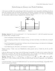
Definition 3.1. Using the notation introduced above, let<br />
⎧<br />
⎨ Z u−⃗e1 Z u+⃗e1 Z u+⃗e2 for x⃗e 1 + 0⃗e 2<br />
∀u ∈ Ω P : P u := Z u−⃗e1 Z u+⃗e1 Z u−⃗e2 for x⃗e 1 + k 2 ⃗e 2<br />
⎩<br />
Z u−⃗e1 Z u+⃗e1 Z u+⃗e2 Z u−⃗e2 otherwise<br />
18<br />
(6)
⎧<br />
⎨ X u−⃗e2 X u+⃗e2 X u+⃗e1 for 0⃗e 1 + y⃗e 2<br />
∀u ∈ Ω T : T u := X u−⃗e2 X u+⃗e2 X u−⃗e1 for k 1 ⃗e 1 + y⃗e 2<br />
⎩<br />
X u−⃗e1 X u+⃗e1 X u+⃗e2 X u−⃗e2 otherwise<br />
∀ (7)<br />
We call P u a plaquette operator, and T u a star operator. As already suggested<br />
by their definition, we will place P operators in Ω P and T operators in Ω T .<br />
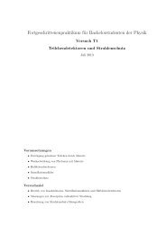
See figure 1<br />
Figure 1: The generators <strong>of</strong> the surface code. The red circles represent the<br />
qubits: Ω even , the white squares represent the plaquette operators: Ω P , and<br />
the black stars represent the star operators: Ω T .<br />
Remark 3.2. Set S := 〈P u , T v | u ∈ Ω P , v ∈ Ω T 〉 ≤ P n . Then S is a<br />
stabilizer group, and thus defines a stabilizer code on the n qubits on Ω even .<br />
Pro<strong>of</strong>: From the way we defined the operators, we know that there are no<br />
overall factors involved, and we thus only have to prove that S is abelian.<br />
To do that, observe first that all operators <strong>of</strong> the same type commute with<br />
each other, since the P operators only have Z Pauli operators, and the T<br />
ones similarly only have X Pauli operators. We then only have to focus on<br />
the commutator <strong>of</strong> P u and T v for all u ∈ Ω P , v ∈ Ω T , and only when there is<br />
overlapping in their support (otherwise they trivially commute). It is easy to<br />
see, that when these operators overlap, they always do so in an even number<br />
<strong>of</strong> sites, and thus commute (see figure 1).<br />
Now that we know that S is a stabilizer group and defines a code, we can<br />
try to analyze it a bit. We will restrict here to the dimension <strong>of</strong> the code.<br />
Further analysis -like the minimal distance - can be found in [1].<br />
Proposition 3.3. For any k 1 , k 2 the 2D surface code with open boundary<br />
conditions encodes a single qubit.<br />
19
We will prove this using theorem 2.20. For this, we first need to find a set<br />
<strong>of</strong> independent generators for the stabilizer group. We will start with the set<br />
we have now: G := {P u | u ∈ Ω P } ∪ {T v | v ∈ Ω T }. By the very definition<br />
<strong>of</strong> the code, this set G generates the stabilizer group S = 〈G〉. We would<br />
like to find an independent subset <strong>of</strong> G, and to do this, we simply look for<br />
linear dependencies in symplectic notation: Let ϕ : S → F 2n<br />
2 be the group<br />
homomorphism that maps S to its symplectic notation. By definition, the<br />
set <strong>of</strong> vectors ϕ(G) is linearly independent if the following equation has no<br />
solution other than a u = 0 ∀ u ∈ Ω odd :<br />
0 = ∑<br />
a u ϕ(P u ) + ∑<br />
ϕ is an homomorphism<br />
{}}{<br />
a v ϕ(T v ) = ϕ( ∏<br />
u∈Ω P v∈Ω T<br />
∏<br />
Pu<br />
au<br />
T av<br />
u∈Ω P v∈Ω T<br />
v ) (8)<br />
∏<br />
v∈Ω T<br />
T av<br />
v ∈ Ker(ϕ). It<br />
This means nothing more than that ∏ u∈Ω P<br />
Pu<br />
au<br />
is easy to see that for the sympletic notation for the whole Pauli group<br />
˜ϕ : P n → F 2n<br />
2 the kernel is Ker( ˜ϕ) = {±iI, ±I}, since ˜ϕ(A) = 0 means that<br />
the exponent in all X i and Z i is 0. Since S ∩ Ker( ˜ϕ) = {I}, it must be that<br />
∏ ∏<br />
Pu<br />
au<br />
Tv av<br />
= Id (9)<br />
u∈Ω P v∈Ω T<br />
We know that the P u are only Z-type operators, and the T u are only X-type.<br />
Therefore, products <strong>of</strong> P u ’s cannot be the inverse <strong>of</strong> products <strong>of</strong> T v ’s and<br />
vice-versa, which means that equation 9 has to hold separately for both T<br />
and P operators:<br />
I P := ∏<br />
u = I (10)<br />
I T := ∏<br />
u∈Ω P<br />
P au<br />
v∈Ω T<br />
T av<br />
v = I (11)<br />
If I P = I, it means that it acts on every qubit as the identity, we can hence<br />
look at the qubits directly: Consider the site at the origin (⃗0): The only P<br />
operator acting on it is P ⃗e1 which acts as a Z on ⃗0: If I P is to act as the<br />
identity on ⃗0, the exponent <strong>of</strong> P ⃗e1 , a ⃗e1 must be 0. If we go on with the next<br />
qubit in that direction, the one at 2⃗e 1 , is acted upon by two P operators: P ⃗e1<br />
and P ⃗e3 , which act both with a Z on the qubit at 2⃗e 1 . Since, however, a ⃗e1 = 0,<br />
it means that a ⃗e3 must be it too, otherwise I P would act as a Z on the qubit<br />
at 2⃗e 1 . We can go on like this and see that all exponents for this row must<br />
be 0, i.e. a (2k+1)⃗e1 = 0, k = 0, 1, 2, . . .. We go on to the next column, starting<br />
with the qubit at u = ⃗e 1 + ⃗e 2 : The P operators acting on this are P ⃗e1 and<br />
P ⃗e1 +2⃗e 2<br />
. A similar reasoning, since we know that a ⃗e1 = 0, yields a ⃗e1 +2⃗e 2<br />
= 0.<br />
20
In a similar fashion we can go on for all P u , u ∈ Ω P to show that a u = 0. From<br />
an analogous argument we can see that the same holds for all T v , v ∈ Ω T , and<br />
hence, the generator set G is already independent! It is a matter <strong>of</strong> simple<br />
combinatorics to see that |Ω odd | = 2k 1 k 2 + k 1 + k 2 = |Ω even | − 1 = n − 1.<br />
Theorem 2.20 immediately yields the statement: the surface code encodes<br />
k = n − (n − 1) = 1 qubits.<br />
This code is called the surface code with open boundary conditions since<br />
we assume that the end points <strong>of</strong> the code are open, and do not interact with<br />
anything else besides their inner neighbours in the lattice. If we identify the<br />
points in the end with the beginning, i.e. look at the points modulo the<br />
length: ˜Ω = {(x mod k1 )⃗e 1 + (y mod k 2 ⃗e 2 | x, y ∈ Z} then we get what is<br />
called the toric code with periodic boundary conditions. From this identification<br />
it is also clear why the code is called toric code. With an argument<br />
similar to proposition 3.3 it can be shown that the toric code with periodic<br />
boundary conditions always encodes 2 qubits.<br />
3.2 Self-correcting Quantum Memory<br />
The main goal <strong>of</strong> quantum error correction is, <strong>of</strong> course, to produce codes that<br />
can be used on a quantum computer. One very important direct application<br />
for codes is storage. We want to be able to reliably store and retrieve data,<br />
and on a quantum computer, qubits. If we have any kind <strong>of</strong> error correcting<br />
codes, even codes which immediately require an active process <strong>of</strong> error<br />
correction (usually designed for transmitting data over a faulty medium), we<br />
can find a way to store data. We simply actively do the error correction<br />
with some regularity which would depend on the code and the medium, and<br />
get a reliable way to store. This, however, has a great disadvantage: active<br />
error correction requires active use <strong>of</strong> diverse technologies: gates to do the<br />
error correction which wear down with time, measurements <strong>of</strong> syndromes,<br />
etc, all <strong>of</strong> which make it more complex and limit the useful life <strong>of</strong> the storage<br />
medium.<br />
There is another way <strong>of</strong> reliably storing data, which can be more longterm<br />
and is in principle more energy-efficient: a self-correcting memory. The<br />
main idea behind a self-correcting quantum memory would be for it to be a<br />
quantum code, which after being perturbed, naturally tends to return to the<br />
original codeword, thus correcting the error ’by itself’. The feasibility <strong>of</strong> such<br />
a self-correcting quantum memory in a 3-dimensional geometrical quantum<br />
code is still an open problem [9], and is the main motivation for the codes<br />
studied in this thesis.<br />
21
3.3 The STS model<br />
Our first approach to finding a self-correcting quantum memory will be the<br />
restriction to a certain class <strong>of</strong> geometrical quantum codes. We will study<br />
codes embedded in a 3-dimensional lattice, for which we will assume periodic<br />
boundary conditions. We will make further assumptions about the codes we<br />
study, assumptions which, however, have a physical motivation.<br />
• Locality:<br />
As discussed at the beginning <strong>of</strong> this section, one <strong>of</strong> the main assumptions<br />
we make on most geometrical quantum codes is locality. If geometrical<br />
quantum codes should result from interactions between the<br />
qubits, it is very reasonable to assume they will do so only locally. We<br />
will formally define this as a restriction on the size <strong>of</strong> the support <strong>of</strong><br />
the stabilizer group elements, which we will require to be constant; in<br />
particular, independent <strong>of</strong> the size <strong>of</strong> the lattice (O(1)).<br />
• <strong>Translation</strong>-Symmetry:<br />
The next assumption we will make is translation symmetry. This basically<br />
means that the code ’looks’ the same from every point in the<br />
lattice: a physical symmetry <strong>of</strong> the code, which is a plausible assumption.<br />
A more formal definition will be given in section 4.<br />
• Scale-Symmetry:<br />
The last assumption is that <strong>of</strong> scale-symmetry <strong>of</strong> the code space dimension;<br />
this means that the code space dimension should not depend<br />
on the size <strong>of</strong> the lattice. A good motivation for this comes from the<br />
intuition that there is a trade<strong>of</strong>f between the number <strong>of</strong> encoded qubits<br />
and the minimal distance <strong>of</strong> the code [11]. For this reason ”it may be<br />
legitimate to limit our considerations to the cases where the number <strong>of</strong><br />
logical qubits k remains small when the system size increases” [9].<br />
This assumption is probably the least well-founded <strong>of</strong> the three, and<br />
while reasonable, I would argue is not an assumption that has to be<br />
made. In a search for any plausible self-correcting quantum memory,<br />
finding a bad code - with a small distance, and/or not coding many<br />
qubits - is still better than no code at all.<br />
We call stabilizer codes which satisfy these three conditions STS codes (for<br />
<strong>Stabilizer</strong>s with <strong>Translation</strong> and Scale symmetries), and note that it is in fact<br />
a very large class <strong>of</strong> codes.<br />
22
Example 3.4. The toric code with periodic boundary conditions is an STS<br />
code: From the stabilizers we immediately see both locality and translationinvariance<br />
<strong>of</strong> the stabilizers. The analysis <strong>of</strong> the code space dimension (which<br />
is always 4, for 2 qubits) immediately satisfies the third condition.<br />
3.4 A Classic Self-Correcting Memory And The Energy<br />
Barrier<br />
Now that we have a first model to search for self-correcting memory, it would<br />
be good to also get a feel for what a self-correcting quantum memory is, and<br />
how it can work. To do this we will start with an example for a classically<br />
self-correcting memory.<br />
In an L × L lattice consider the following 2D Ising model:<br />
H = − ∑ x,y<br />
Z x⃗e1 +y⃗e 2<br />
Z (x+1)⃗e1 +y⃗e 2<br />
− Z x⃗e1 +y⃗e 2<br />
Z x⃗e1 +(y+1)⃗e 2<br />
The ground space <strong>of</strong> this Hamiltonian is spanned by |0 . . . 0〉 and |1 . . . 1〉<br />
and can thus be used for storing a classical bit: 1 ↦→ |1 . . .〉, 0 ↦→ |0 . . .〉. If we<br />
use this system as a memory, it will interact with the environment with time<br />
and produce errors. For these errors to make an error in the encoded classical<br />
bit, they have to take |0 . . .〉 to |1 . . .〉 or vice-versa. This means errors will<br />
have to flip all the spins (which are the qubits in this particular example) from<br />
|0〉 to |1〉 or vice-versa, which requires an energy that is O(L). For large L<br />
this is a large energy barrier that has to be be crossed by the error-producing<br />
interactions (assumed to be mostly <strong>of</strong> thermic nature) in order to make an<br />
error on the encoded bit. In most cases, before the system has gathered<br />
enough energy from the environment to corrupt this bit, natural thermal<br />
dissipation has brought the system back to its ground state, correcting the<br />
errors that occurred. In this way, the system corrects the errors by itself.<br />
We are interested in the same principle for quantum codes: where the code<br />
is the ground state and there is an energy barrier separating two ground states<br />
in such a manner, that the code will mostly correct itself before making an<br />
error (logical operator) on the encoded data. This energy barrier is central<br />
to the concept <strong>of</strong> a self-correcting memory, as it has to be ’large’ for selfcorrection<br />
to be feasible. We will take here ’large’ to mean not O(1), but at<br />
least O(L q ) for some q ∈ R, and while in principle a small q would be good<br />
as well, we do rather look for a code with energy barrier that is O(L).<br />
Theorem 3.5 (Yoshida). There exists no 3-dimensional STS code that can<br />
work as a self-correcting quantum memory, i.e. all 3-dimensional STS codes<br />
have an energy barrier that is O(1). A pro<strong>of</strong> can be found in [9].<br />
23
3.5 The Haah <strong>Code</strong><br />
Noteworthy <strong>of</strong> mentioning is that in the examples specifically studied by<br />
Yoshida in [9], as he himself remarks, the codes have ”string-like” logical<br />
operators. This means operators with support that looks like a string on the<br />
lattice: for a more formal definition see [4]. These string-like operators make<br />
the energy barrier O(1) since only the boundaries <strong>of</strong> the string affect the<br />
energy. This might lead to an idea <strong>of</strong> how to search for codes which might<br />
be a self-correcting quantum memory: codes without such operators.<br />
An example <strong>of</strong> a code without string-like logical operators was proposed<br />
by Haah in [3].<br />
In the next section we will analyze this code, in particular it’s code space<br />
dimension as a function <strong>of</strong> the lattice size L. We will see that it depends<br />
very strongly on L and for that reason it is not scale-invariant, hence, not<br />
an STS code. In fact, in [3] Haah shows that this code has no string-like<br />
logical operators. While this does not mean that the code is a self-correcting<br />
quantum memory, Yoshida’s theorem ( 3.5) does not apply, and it certainly<br />
is a plausible candidate for a 3-dimensional self-correcting quantum memory!<br />
24
4 <strong>Translation</strong>-<strong>Invariant</strong> <strong>Stabilizer</strong> <strong>Code</strong>s<br />
In section 3 we got an introduction to geometric codes, and the problem <strong>of</strong><br />
finding a self-correcting quantum memory. From theorem 3.5 we know that<br />
STS models are not the way to go in 3 dimensions, and mentioned the Haah<br />
code, which ignores the third condition on STS codes, namely that <strong>of</strong> scale<br />
invariance. In this section we will further pursue this model, translation<br />
invariant, local geometrical stabilizer codes, without any restriction on the<br />
dependence <strong>of</strong> the number <strong>of</strong> encoded qubits on the size <strong>of</strong> the lattice.<br />
4.1 <strong>Stabilizer</strong> codes on a lattice with periodic boundary<br />
conditions<br />
We begin by formalizing a few <strong>of</strong> the concepts seen on section 3.<br />
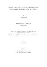
Definition 4.1. Let B = (⃗e 1 , · · · , e n ) ⊂ R n be a Basis <strong>of</strong> R n . Here, we<br />
will assume B is an orthonormal basis, although it is not necessary. We call<br />
˜L = { ∑ n<br />
i=1 a ie i | a i ∈ Z} =: 〈⃗e 1 , · · · e n 〉 Z a lattice with basis B. We can think<br />
<strong>of</strong> this as a discrete arrangement <strong>of</strong> points which differ by multiple integers<br />
<strong>of</strong> the basis vectors (see fig. 2).<br />
Figure 2: Part <strong>of</strong> a lattice in R 2<br />
We will slightly change the ’embedding’ we saw on section 3.1: we will<br />
picture a qubit on every point <strong>of</strong> the lattice. There is <strong>of</strong> course no reason<br />
to restrict the number <strong>of</strong> qubits per point(also called site) to one; we could<br />
include m qubits per site and just label them from 1 to m. Since the lattice<br />
defined on 4.1 has infinitely many points, and we would want to consider finite<br />
codes, we have to include boundary conditions as well. We will consider<br />
25
periodic boundary conditions: we consider points to be the same if they<br />
differ by a multiple <strong>of</strong> some number l i in the direction e i , i.e. for some<br />
l = (l 1 , · · · , l n ) let L := ˜L/lZ := { ∑ n<br />
i=1 (a i mod l i )e i } be the factor lattice<br />
<strong>of</strong> ˜L modulo lZ or the Lattice ˜L with periodic boundary conditions l. Once<br />
we have labeled the qubits, it is easier to specify some classes <strong>of</strong> stabilizer<br />
generators. Note that this definition is not exactly the same as is usual in<br />
mathematics, but it is easier to understand and the resulting structures are<br />
equivalent.<br />
Definition 4.2.<br />
• Let C be a stabilizer code in the lattice with periodic boundary conditions<br />
L with stabilizer group S. We call C a translation-invariant code<br />
iff for each s ∈ S and each ⃗t ∈ L there exists an s ′ ∈ S which differs<br />
by ⃗t, i.e. : for each ⃗r ∈ L s acts on the qubit labeled by ⃗r as s ′ acts on<br />
that labeled by ⃗r + ⃗t. If there is more than one qubit per site this has<br />
to hold for each <strong>of</strong> the qubits independently.<br />
• For an operator A ⃗ 0 ∈ P n we define the translation-invariant generated<br />
group as the group including all translations <strong>of</strong> A : {A ⃗ 0+⃗t | ⃗t ∈ L}.<br />
As this whole section is motivated by it, we will dive in directly into<br />
the Haah code from section 3.5. We will develop the formalism and the<br />
method for calculating the dimension alongside applying it to the Haah code.<br />
Consider the 3D-lattice L with periodic boundary conditions l 1 = l 2 = l 3 =:<br />
l ∈ Z and two qubits per site (m = 2). We will label the qubits by ⃗v, j;<br />
j = 1, 2, v = ∑ 3<br />
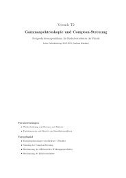
i=1 (a i mod l i )⃗e i . Consider then the two stabilizers<br />
˜X ⃗ 0 = X ⃗0,1 X ⃗0,2 X ⃗e 1 ,2X ⃗e2 ,2X ⃗e3 ,2X (⃗e1 +⃗e 2 ),1X (⃗e2 +⃗e 3 ),1X ⃗(⃗e1 +⃗e 3 ),1<br />
(12)<br />
and ˜Z ⃗ 0 = Z (⃗e 1 +⃗e 2 +⃗e 3 ),1Z (⃗e1 +⃗e 2 +⃗e 3 ),2Z ⃗e1 ,2Z ⃗e2 ,2Z ⃗e3 ,2Z (⃗e1 +⃗e 2 ),1Z (⃗e2 +⃗e 3 ),1Z ⃗(⃗e1 +⃗e 3 ),1<br />
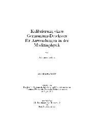
(13)<br />
See figure 3.<br />
We want this to be a translation-invariant code, so for each translation<br />
⃗t ∈ L we take<br />
˜X ⃗ 0+⃗t := X (⃗0+⃗t),2 X (⃗e 1 +⃗t),1 X (⃗e 3 +⃗t),1 X (⃗e 3 +⃗t),2 X (⃗e 2 +⃗t),1 X (⃗e 1 +⃗e 3 +⃗t),2 X (⃗e 2 +⃗e 3 +⃗t),2 X (⃗e 1 +⃗e 2 +⃗e 3 +⃗t),1<br />
and ˜Z ⃗ 0+⃗t<br />
accordingly into S. One easily calculates from figure 3 that all<br />
generators commute, and since there are no overall factors on the generators,<br />
it is easy to see that this is indeed a stabilizer code (−I /∈ S).<br />
Questions about the properties <strong>of</strong> this code immediately arise: Do they<br />
encode qubits? If so, how many? And what is the minimal distance? In<br />
26
Figure 3: Haah code generators<br />
this thesis we will address the first two questions, which are in some sense<br />
more fundamental. The number <strong>of</strong> encoded qubits is <strong>of</strong> course also highly<br />
interesting for this code as it will turn out to depend very much on L, breaking<br />
the scale-invariance and making the Haah code a non-STS code. The minimal<br />
distance, however, is still <strong>of</strong> extreme importance as it is a measure <strong>of</strong> the<br />
error-correcting properties <strong>of</strong> the code. It is a good point for further study.<br />
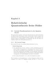
Figure 4: Boundary conditions for l = 2: the points marked with the same<br />
figures (including colour) are identified to be the same<br />
Example 4.3. We begin examining the Haah code in the smallest non-trivial<br />
lattice: l = 2. This code can be thought <strong>of</strong> as an arrangement <strong>of</strong> cubes like<br />
the one on figure 3, but with the boundary conditions that identify the cubes<br />
as marked on figure 4. So, for instance, going from ⃗e 1 to the right once<br />
2⃗e 1 ≡ 0⃗e 1 (mod2) takes you back to ⃗0. Hence, the lattice L has 8 distinct<br />
points, and two qubits per point, for a total <strong>of</strong> 16 qubits. An important<br />
27
observation, and one which applies to the Haah code in general is that it is<br />
a CSS code. This also means that the stabilizer group is a direct product <strong>of</strong><br />
two smaller subgroups, X and Z, which are generated by the X and Z type<br />
operators respectively. We see that ˜Z ⃗ 0 is the same as ˜X ⃗ 0<br />
with Z’s instead <strong>of</strong><br />
X’s, except for a reflection along the ⃗e 1 + ⃗e 2 + ⃗e 3 -axis. This means however,<br />
that the subgroups will be isomorphic (the reflection is just a renaming <strong>of</strong> the<br />
points) and will have the same number <strong>of</strong> independent generators. For this<br />
reason it is enough to determine the number <strong>of</strong> independent generators k for<br />
X and forget about Z, the number <strong>of</strong> qubits encoded by the code altogether<br />
will be given by n − 2k.<br />
If we label the points as in figure 5, and use the short notation (i, j) for X i,j ,<br />
we get the following table for all generators:<br />
Figure 5: Labeling <strong>of</strong> the qubit sites for the Haah code generator ˜X<br />
translation ⃗t <strong>Stabilizer</strong>s in short form (i,j)<br />
0 (1,2)(2,1)(3,1)(3,2)(4,2)(5,1)(7,2)(8,1)<br />
⃗e 1 (3,2)(4,1)(1,1)(1,2)(2,2)(7,1)(5,2)(6,1)<br />
⃗e 2 (2,2)(1,1)(4,1)(4,2)(3,2)(6,1)(8,2)(7,1)<br />
⃗e 3 (5,2)(6,1)(7,1)(7,2)(8,2)(1,1)(3,2)(4,1)<br />
⃗e 1 + ⃗e 2 (4,2)(3,1)(2,1)(2,2)(1,2)(8,1)(6,2)(5,1)<br />
⃗e 1 + ⃗e 3 (7,2)(8,1)(5,1)(5,2)(6,2)(3,1)(1,2)(2,1)<br />
⃗e 2 + ⃗e 3 (6,2)(5,1)(8,1)(8,2)(7,2)(2,1)(4,2)(3,1)<br />
⃗e 1 + ⃗e 2 + ⃗e 3 (8,2)(7,1)(6,1)(6,2)(5,2)(4,1)(2,2)(1,1)<br />
Table 2: <strong>Stabilizer</strong> generators for l=2<br />
28
If we then write this in symplectic notation, we get the matrix:<br />
⎛<br />
⎞<br />
0 1 1 0 1 1 0 1 1 0 0 0 0 1 1 0<br />
1 0 0 1 0 1 1 1 0 0 1 0 1 0 0 1<br />
1 0 0 0 0 1 1 0 0 1 1 0 1 1 0 1<br />
1 1 0 1 0 1 1 0 0 1 1 0 1 0 0 0<br />
0 0 1 0 1 0 0 1 1 0 0 1 0 1 1 1<br />
⎜ 0 1 1 1 1 0 0 1 1 0 0 1 0 0 1 0<br />
⎟<br />
⎝ 0 1 1 1 1 0 0 1 1 0 0 1 0 0 1 0 ⎠<br />
1 0 0 1 0 0 1 0 0 1 1 1 1 0 0 1<br />
This is a rank 5 matrix over F 2 , which means that there is only 5 independent<br />
generators, hence altogether 10 with Z, for a total <strong>of</strong> 16 − 10 = 6<br />
encoded qubits.<br />
This was a pretty tedious calculation and this is only the smallest example!<br />
Luckily, while doing the calculation we can already see hints that there<br />
is an easier way <strong>of</strong> doing it. We first note that the translations just move<br />
the single qubit Pauli operators from the stabilizers around. By labeling<br />
the points in the lattice from 1 to 8 we saw that each translation can be<br />
understood as a simple permutation <strong>of</strong> those 8 points. In the language <strong>of</strong><br />
group theory: the abelian group (with respect to addition) G := L acts on<br />
the Pauli group, and the generators are the orbits <strong>of</strong> ˜X ⃗ 0 and ˜Z ⃗ 0<br />
. We can use<br />
this realization to generalize this method for an arbitrary L:<br />
We noted above that the lattice L acts as a permutation group on the<br />
Pauli group elements. If we number the lattice points in a clever way, the<br />
action will be very easy to describe. It is a simple matter to implement said<br />
action, and input the first generator, to generalize the method we used on<br />
example 4.3 and for it to work on the code for a general size. In principle<br />
we are done: this whole approach reduces the problem to linear algebra, and<br />
calculating the rank <strong>of</strong> a matrix over F 2 . Unfortunately, this is a matrix with<br />
size O(l 6 ), and it soon becomes incalculable: Only for l = 15 the matrix<br />
has around 22 million entries and it took about 45 minutes to calculate it<br />
and its rank on an Intel i3 Pc with an implementation using a computer<br />
algebra system (which can definitely be improved upon, but gives an idea <strong>of</strong><br />
the scaling with the size <strong>of</strong> the problem).<br />
4.2 <strong>Translation</strong>-invariant codes on lattices as factor<br />
rings <strong>of</strong> polynomial rings<br />
Fortunately, we can recognize more structure on the codes. We will try to<br />
develop the analysis <strong>of</strong> the structure directly in a general fashion, so it can<br />
29
e used for any translation-invariant stabilizer codes on a lattice. We know<br />
that the stabilizer group is a vector space over R := F 2 , making it with the<br />
action <strong>of</strong> G what is called an RG-Module, where RG is the so-called group<br />
ring.<br />
Definition 4.4. Let G be a finite group and R be a commutative ring with<br />
unity. Set the ring RG := { ∑ g∈G r gg | r g ∈ R} with the product in the<br />
group extended such, that the distributive law holds. Then RG is called the<br />
group ring <strong>of</strong> G over R. A field K is also a ring, so that the group ring KG<br />
is also an algebra over the field K.<br />
The following is partially based on unpublished notes by Jeongwan Haah:<br />
Let G be a finite abelian group, and RG its group ring over R = F 2 . G<br />
will be the lattice, and although the group needs not be abelian for this<br />
analysis, a lattice should always be. At each g ∈ G we place m ∈ N<br />
qubits. Up to an overall phase, we can then express every Pauli operator as<br />
X f1 ,1 · · · X fm,mZ g1 ,1 · · · X gm,m, where f i , g i ∈ RG for all i ∈ m express where<br />
on the lattice the operator is supported. Note that this notation differs from<br />
the one introduced above, but there is no danger <strong>of</strong> confusion, as it shall be<br />
immediately clear from the context what it means (we will use this notation<br />
only when talking about group ring elements). For example, the operator<br />
P ⃗e1 = Z ⃗ 0 Z ⃗e 1 +⃗e 1<br />
Z ⃗e1 +⃗e 2<br />
from the surface code (section 3.1) would be written<br />
as X f Z g (we leave the qubit numbering out, since it is one qubit per site),<br />
with f = 0, g = ⃗0 + ⃗e 1 ⃗e 1 + ⃗e 1 ⃗e 2 . Note that we write addition in the lattice<br />
multiplicatively, as it is the operation in the group G = L, to differentiate it<br />
from addition in the group ring RG.<br />
Remark 4.5. Since the lattice G is a finite abelian group, by the structure<br />
theorem <strong>of</strong> finitely generated abelian groups (see, for example [7]) it is isomorphic<br />
to ˜L/(l 1 , . . . , l n )Z for some l 1 , . . . , l n ∈ N. Hence, it is with loss <strong>of</strong><br />
generality that we can assume that structure for the lattice. In particular,<br />
this means that, for example, changing the way the boundary conditions are<br />
set will not change the structure <strong>of</strong> the code: The lattice will always be an<br />
abelian group, and structurally it would only mean a renaming <strong>of</strong> the points.<br />
Remark 4.6. As a F 2 vector space, an element <strong>of</strong> RG is the same as the Pauli<br />
group element in symplectic notation. In particular, stabilizer groups in RG<br />
have an F 2 <strong>Dimension</strong> equal to the uniquely defined number <strong>of</strong> independent<br />
generators.<br />
At this point, it might be useful to do a summary <strong>of</strong> the identifications<br />
with the group ring RG and Pauli group elements: As in remark 4.6, we can<br />
30
think <strong>of</strong> an element <strong>of</strong> RG simply as the Pauli group element in symplectic<br />
notation. RG has two operations, product and sum:<br />
• The sum in RG is the sum over F 2 in symplectic notation. For the<br />
Pauli operators it is the same as the product in the Pauli group.<br />
• The product with an element <strong>of</strong> g ∈ G ⊂ RG (as opposed to a sum <strong>of</strong><br />
such) is a translation <strong>of</strong> the Pauli element with the ’lattice vector’ g.<br />
• From those identifications above, we can understand the product in<br />
RG: RG ∋ r = ∑ g∈G a gg; a g ∈ R = F 2 . If r ≠ 0, multiplying the<br />
Pauli group element d ∈ RG with r means that for each a g ≠ 0 we<br />
take<br />
∑<br />
the translation gd and multiply all those in the Pauli group: rd =<br />
g,a gd.<br />
g≠0<br />
• There is a special case which has been left out: r = 0. 0 /∈ G ⊂ RG.<br />
Product with 0 can be understood as a ’translation to nowhere’, since<br />
it takes the Pauli group element to the identity in the Pauli group.<br />
Alternatively, one can understand 0d = d0, d ∈ RG as a sum <strong>of</strong> the<br />
translations <strong>of</strong> d for the identity, as above.<br />
A further thing to notice is then the following: Let d ∈ RG be a Pauli<br />
group element. Then, the translation-invariant generated group is the ideal<br />
(d) = {rd | r ∈ RG}: We first take all translations <strong>of</strong> d: {gd | g ∈ G ⊂ RG},<br />
and then take the group generated by them, i.e. all products in the Pauli<br />
group <strong>of</strong> such elements: { ∑ g∈H<br />
gd | H ⊂ G ⊂ RG} = (d).<br />
Remark 4.7. Let I : RG → RG, g ↦→ g := g −1 be the homomorphism<br />
which maps group elements to their inverses(since G is abelian, it is indeed a<br />
homomorphism). Set further for R ∋ r = ∑ g∈G r gg, tr(r) := r 1 ∈ F 2 , where<br />
1 is the unit element in G. Then, the symplectic product <strong>of</strong> two Pauli group<br />
elements P = X f1 ,1 · · · X fm,mZ g1 ,1 · · · X gm,m,<br />
P ′ = X f ′<br />
1 ,1 · · · X f ′ m ,mZ g ′<br />
1 ,1 · · · X g ′ m ,m is given by<br />
[P, P ′ ] =<br />
m∑<br />
m∑ ∑<br />
[X fi ,iZ gi ,i, X f ′<br />
i ,iZ g ′<br />
i ,i] = (f i ) h (g i) ′ h + (f i) ′ h (g i ) h (14)<br />
i=1<br />
=<br />
i=1 h∈G<br />
m∑<br />
m∑<br />
tr(f i g i ′ + f i ′ g i) = tr( f i g i ′ + f i ′ g i) (15)<br />
i=1<br />
i=1<br />
where the 2. equality follows from [1] and (f i ) h denotes the coefficient <strong>of</strong> h<br />
<strong>of</strong> f i .<br />
31
Definition 4.8 (CSS <strong>Code</strong>). Set for d 1 , d 2 ∈ RG, X = 〈X rd1 ,1 X rd 2 ,2 | r ∈<br />
RG〉 and Z = 〈Z rd1 ,1Z rd2 ,2 | r ∈ RG〉 (m = 2 qubits per site). Then<br />
S = X × Z is a stabilizer group, since from eqn. all generators commute and<br />
by construction there is no phase factors, hence −I /∈ S.<br />
It is worth noting that this way we define a general class <strong>of</strong> translationinvariant<br />
CSS codes, including the Haah code, but the results from later do<br />
not need this CSS structure. To show the main result <strong>of</strong> this thesis, we will<br />
need a few mathematical definitions and technical results:<br />
Remark 4.9.<br />
• The function tr defines a bilinear form (·, ·) : R × R → F 2 through<br />
(a, b) := tr(ab). It can be easily seen that the Gram-Matrix <strong>of</strong> this<br />
bilinear form in the basis G is the identity, thus, (·, ·) is non-degenerate<br />
and symmetric.<br />
• For a subspace V <strong>of</strong> RG let V ⊥ := {r ∈ RG | (r, v) = 0 for all v ∈<br />
V } be the orthogonal complement <strong>of</strong> V with respect to (·, ·). Then<br />
(V ⊥ ) ⊥ = V .<br />
• Let RG ∗ := {ϕ : RG → R | ϕ is linear} be the dual space <strong>of</strong> RG. Then<br />
we have a canonical (base independent) isomorphism between RG and<br />
RG ∗ given by RG ∋ a ↦→ (a, ·) ∈ RG ∗ .<br />
Definition 4.10. Let R,S be two commutative rings with unity, and ϕ :<br />
R → S be a ring homomorphism. Set Im(ϕ) := {ϕ(r) | r ∈ R}. Then the<br />
Cokernel <strong>of</strong> ϕ is defined as:<br />
Coker(ϕ) := S/Im(ϕ) = {s + Im(ϕ) | s ∈ S} (16)<br />
Lemma 4.11. Let G be a finite abelian group, R := F 2 G be its group ring<br />
and d 1 , . . . , d m ∈ R. Further let I, J ⊳ R be the two ideals in R defined by<br />
I := ⋂ m<br />
i=1 Ann(d i) := ⋂ m<br />
i=1 {r ∈ R | rd i = 0} = {r ∈ R | rd i = 0 for all i ∈<br />
m}, and J := (d 1 , . . . , d m ) := { ∑ m<br />
i=1 r id i | r i ∈ R for all i ∈ m}. 1 Then<br />
R/J ∼ = I as vector spaces, which is equivalent to dim F2 (R/J) = dim F2 I.<br />
Pro<strong>of</strong>: Consider the following mapping:<br />
ϕ : R → I ∗ , R ∋ r ↦→ r|I ∗ = (i ↦→ (r, i)∀i ∈ I) ∈ I ∗<br />
1 If you have never seen the notation Ann(d i ) just don’t worry about it, take it as just<br />
a name<br />
32
We want to show the assertion using the fundamental theorem on homomorphisms.<br />
If we can show that ϕ(R) = I ∗ and Ker(ϕ) = J (see fig. 6), then it<br />
immediately follows from it that R/J ∼ = I ∗ as F 2 -algebras, and this implies<br />
the assertion for vector spaces as well. Since (·, ·) is non-degenerate, we know<br />
that ∗ : I → I ∗ , i ↦→ i ∗ = (i, ·) is a surjective mapping, and since I ⊆ R, it is<br />
immediately clear that ϕ is surjective as well, and hence: ϕ(R) = I ∗ . Now<br />
we turn to Ker(ϕ) = {r ∈ R | (r, ·) |I ≡ 0} = {r ∈ R | (r, i) = 0 ∀ i ∈ I} = I ⊥ .<br />
This means we only need to show that I ⊥ = J. Note that since (·, ·) is nondegenerate,<br />
rd i = 0 ⇔ (rd i , g) = 0∀g ∈ G, as G is a basis <strong>of</strong> RG. It follows<br />
then that<br />
Ann(d i ) = {r ∈ R | rd i = 0} = {r ∈ R | (rd i , g) = tr(rd i g) (17)<br />
= tr(grd i = (gr, d i ) = 0 for all g ∈ G} = (d i ) ⊥ (18)<br />
Since Ann(d i ) is an ideal, we can forget about the g, as rd i = 0 ⇒ grd i = 0,<br />
which gives the last equality from equation 18. We get that:<br />
m⋂<br />
m⋂<br />
m∑<br />
I = Ann(d i ) = (d i ) ⊥ = ( (d i )) ⊥ = J ⊥<br />
i=1<br />
i=1<br />
It follows that Ker(ϕ) = I ⊥ = J and since I is an isomorphism, dim F2 R/J =<br />
dim F2 R/J = dim F2 I.<br />
i=1<br />
Figure 6: Fundamental theorem on homomorhisms, here ϕ is surjective as<br />
indicated by the double arrow, and τ is the canonical homomorphism: τR →<br />
R/J, r ↦→ r + J<br />
Definition 4.12. The free group on {x, y} is defined as follows:<br />
Fr({x, y}) := {w | w is a finite product <strong>of</strong> {x, y, x −1 , y −1 }}<br />
whilst we consider two such finite products to be the same if they differ<br />
by pairs <strong>of</strong> inverse elements at some point. For instance xxyy ≠ xyyx =<br />
xyy −1 yyx −1 xx(= xy(y −1 y)y(x −1 x)x). Any group G that can be generated<br />
by two elements G = 〈g 1 , g 2 〉 can be ’presented’ as a factor group <strong>of</strong> Fr(x, y).<br />
33
The kernel R <strong>of</strong> the mapping x ↦→ g 1 , y ↦→ g 2 is called the relations <strong>of</strong> G and<br />
has exactly the products <strong>of</strong> g 1 , g 2 , expressed in x, y which multiply to 1. If<br />
R is generated by r 1 , . . . , r k we write G ∼ = 〈x, y | r 1 , . . . , r k 〉, this is called a<br />
presentation <strong>of</strong> G. From this definition it should be clear how to generalize<br />
this for n generators x 1 , . . . , x n instead <strong>of</strong> x, y.<br />
Example 4.13. For example, a presentation <strong>of</strong> the 2-dimensional lattice L<br />
as an abelian group: ˜L/(l1 , l 2 )Z, can be found as follows: We know that L<br />
is generated by the two elements ⃗e 1 , ⃗e 2 , so we take those for the mapping:<br />
x ↦→ e 1 , y ↦→ e 2 . We know that e 1 , e 2 commute, so that xyx −1 y −1 should<br />
be a relation (additively in L this means (⃗e 1 + ⃗e 2 ) − (⃗e 2 + ⃗e 1 ) = ⃗0). We<br />
further know the boundary conditions: l 1 ⃗e 1 = l 2 ⃗e 2 = ⃗0, which translate to<br />
x l 1<br />
= 1 = y l 2<br />
, so we should take those two relations as well. It is not hard<br />
to see that we are already done, as we can immediately tell by counting the<br />
number <strong>of</strong> elements in the group with this presentation. So, altogether we<br />
get L ∼ = 〈x, y | xyx −1 y −1 , x l 1<br />
, y l 2<br />
〉.<br />
Remark 4.14. Let K be a field. Then the set <strong>of</strong> all polynomials (<strong>of</strong> finite<br />
degree) in the variables x 1 , . . . , x n and coefficients in K, denoted by<br />
K[x 1 , . . . , x n ], is a commutative ring with unity. This can be read in most<br />
introductory algebra textbooks, for example [7].<br />
Definition 4.15. Let K be a field and R be a K-Algebra, d 1 , . . . , d n ∈ R are<br />
called algebraically independent iff every polynomial f ∈ K[x 1 , . . . , x n ] which<br />
satisfies f(d 1 , . . . , d n ) = 0 is the 0 polynomial, i.e. there exists no non-zero<br />
polynomial which satisfies f(d 1 , . . . , d n ) = 0. Elements d 1 , . . . , d n which are<br />
not algebraically independent are also called algebraically dependent.<br />
Example 4.16. The polynomials x + 1, y 2 + y ∈ K[x, y] are algebraically<br />
independent, which can be seen immediately from degree arguments. On<br />
the other hand, x 2 + 1 and x are not algebraically independent over F 2 ,<br />
since x 2 + 1 + (x + 1) 2 = 0, which means that the non-trivial polynomial<br />
f = x + (y + 1) 2 ∈ F 2 [x, y] satisfies f(x 2 + 1, x) = 0.<br />
Proposition 4.17. Let G be a finite abelian Group, and<br />
〈x 1 , . . . x n | r 1 , . . . r m , x 1 x 2 x −1<br />
1 x −1<br />
2 , x 1 x 3 x −1<br />
1 x −1<br />
3 , . . . , x n−1 x n x −1<br />
n−1x −1<br />
n 〉<br />
be a presentation <strong>of</strong> G. Note that we always get the relations x i x j x −1<br />
i<br />
for abelian groups but we are not interested in them here.<br />
Let further<br />
K be a field. Then the group ring R := KG is isomorphic as a ring to<br />
K[x 1 , . . . , x n ]/(r 1 +1, . . . , r m +1) where K[x 1 , . . . , x n ] where (r 1 , +1 . . . , r m +<br />
1) := { ∑ m<br />
i=1 a i(r i +1) | a i ∈ K[x 1 , . . . , x n ]} denotes the ideal <strong>of</strong> K[x 1 , . . . , x n ]<br />
generated by {r 1 + 1, . . . , r m + 1}. Is I = ⋂ k<br />
i=1 Ann(d i) ⊳ KG for some<br />
d 1 , . . . , d k ∈ KG, then I ∼ = K[x 1 , . . . , x n ]/(r 1 + 1, . . . , r m + 1, d 1 , . . . , d k )<br />
34<br />
x −1<br />
j
Pro<strong>of</strong>: For the first part an isomorphism is given by x i ↦→ x i , which is well defined<br />
since G is abelian. For the second part we will first take the case k = 1.<br />
Look at the mapping ϕ : R → R, r ↦→ rd. We immediately get that Ker(ϕ) =<br />
Ann(d), Im(ϕ) = (d), Coker(ϕ) = R/(d). From the fundamental theorem on<br />
homomorphisms we know Im(ϕ) ∼ = R/Ker(ϕ) = R/Ann(d), which we can<br />
embed in R since Im(ϕ) ⊂ R. We will call this embedding R/Ann(d) ∼ = J ⊳R.<br />
With this embedding we can look at Coker(ϕ) = R/Im(ϕ) ∼ = R/J(” ∼ =<br />
R/(R/Ann(d))”), and R/J ∼ = Ann(d), hence Ann(d) ∼ = Coker(ϕ) = R/(d) ∼ =<br />
K[x 1 , . . . , x n ]/(r 1 +1, . . . , r m +1, d), where the last isomorphy is immediately<br />
clear from the mapping x i ↦→ x i . Now for a general k, we know from prop.<br />
4.11 that R/J ∼ = I, which means in particular from the fundamental theorem<br />
on homomorphisms, that there is a mapping ϕ : R ↦→ R with Im(ϕ) = I and<br />
Ker(ϕ) = J. The rest <strong>of</strong> the argument never explicitly used more <strong>of</strong> I and<br />
J, so it holds for this case as well.<br />
Remark 4.18. Let C be a translation-invariant stabilizer code ’embedded’<br />
on the lattice L = G. Let KG be the group ring over K = F 2 .<br />
Let A 1 , . . . , A k be a set <strong>of</strong> stabilizers such, that the stabilizer group is the<br />
translation-invariant group generated by the A i , as in def. 4.2. Then (up<br />
to a scalar factor, for which we don’t care here) we can write each A i as<br />
X f1 ,1 . . . X fm,mZ g1 ,m . . . Z gm,m. For simplicity <strong>of</strong> the argument we will assume<br />
that k = m = 1; a generalization <strong>of</strong> the result is straightforward. Then we<br />
can write the generator A 1 as X f Z g . But there is no need to separate f and<br />
g: If we define the ring R to be KG 2 = KG ⊕ KG , we can write d ∈ KG 2<br />
for the whole support <strong>of</strong> A 1 (d = f ⊕ g). We can thus write the stabilizer<br />
code S as an ideal I ⊳ R:<br />
I := (d) := {rd | r ∈ R} ⊳ R (19)<br />
The general case with k translation-invariant generators and m qubits per<br />
site simply yields an ideal generated by many elements, on a larger ring:<br />
I = (d 1 , . . . , d k ) := {r 1 d 1 + . . . + r k d k | r 1 , . . . , r k ∈ R = KG 2m } ⊳ R = KG 2m<br />
(20)<br />
Note that this is not necessarily a stabilizer code for any arbitrary d 1 , . . . , d k ;<br />
but (up to a scalar factor) every translation-invariant stabilizer code on a<br />
lattice can be written this way. We can always choose a set <strong>of</strong> generators<br />
˜d 1 , . . . , ˜d l ∈ KG 2 , l ≤ k so, that it is algebraically independent.<br />
Proposition 4.17 gives us, using remark 4.18, a good tool for calculating<br />
the dimension <strong>of</strong> a general translation-invariant code:<br />
35
Theorem 4.19. Let C be a translation-invariant 3D stabilizer code with one<br />
qubit per site, generated translation-invariant from A 1 , . . . , A l as in def. 4.2<br />
and d 1 , . . . , d k be the corresponding algebraically independent ideal generators<br />
as in remark 4.18. Further let K = F 2 and E i := K[x 1 , . . . , x 6 ]/(x l 1<br />
1, x l 2<br />
2 +1, x l 3<br />
3 +1, x l 1<br />
4 +1, x l 2<br />
5 +1, x l 3<br />
6 +1, d i ). Then the F 2 dimension <strong>of</strong> the stabilizer<br />
group S (which is the same as the number <strong>of</strong> independent generators)<br />
is given by Dim S = 2k|G| − ∑ k<br />
i=1 Dim E i.<br />
Pro<strong>of</strong>: We will first prove it for k = 1: Set the mapping ϕ : KG 2 →<br />
KG 2 , r ↦→ rd. The image <strong>of</strong> ϕ is given by Im(ϕ) = {rd | r ∈ KG 2 } = (d) ⊳<br />
KG 2 and the kernel Ker(ϕ) = {r ∈ KG 2 | rd = 0} = Ann(d) ⊳ KG 2 . From<br />
the fundamental theorem on homomorphisms we know that KG 2 /Ann(d) ∼ =<br />
(d). If we look at KG 2 as a F 2 vector space only, an operator in KG 2 is<br />
the same as the operator in symplectic notation. That is why, (d) ∼ = S as F 2<br />
vector spaces (see remark 4.18). On the other hand, we know from prop. 4.17<br />
that E ∼ = Ker(ϕ), which gives the result. For a general k, we change the mapping<br />
to ϕ : KG 2k → KG 2 , (r 1 , . . . , r k ) ↦→ ∑ k<br />
i=1 r id i . The image is Im(ϕ) =<br />
(d 1 , . . . , d k ). The kernel is given by Ker(ϕ) = ⊕ n i=1Ann(d i ). That this is<br />
in the kernel is obvious, that it is the whole kernel is a consequence <strong>of</strong> the<br />
algebraic independence <strong>of</strong> the d i ’s, since an element ∈ Ker(ϕ)\ ⊕ n i=1 Ann(d i )<br />
would immediately yield a non-trivial way <strong>of</strong> combining d 1 , . . . , d k to 0. The<br />
rest is analogous to the case for k = 1.<br />
Using proposition 4.17 it is straightforward to extend theorem 4.19 for m<br />
qubits per site.<br />
Corollary 4.20. Set E := F 2 [x 1 , x 2 , x 3 ]/(x l 1<br />
1 +1, x l 2<br />
2 +1, x l 3<br />
3 +1, d 1 , d 2 ). Then,<br />
for the CSS code defined in 4.8 we have in symplectic notation dim X =<br />
dimZ, and so we get the number <strong>of</strong> independent generators k as: k = 2|G| −<br />
2Dim E ⇒ 2Dim E = 2|G| − k, and so, the number <strong>of</strong> encoded qubits is<br />
given by 2Dim E.<br />
Pro<strong>of</strong>. The pro<strong>of</strong> is almost the same as in theorem 4.19, but we set the<br />
mapping ϕ : KG → KG 2 , r ↦→ rd 1 + rd 2 , and make use <strong>of</strong> the fact that<br />
Dim X = Dim Z, which we can immediately see from their definition.<br />
Theorem 4.19 is a great result. Through it, we have managed to reduce<br />
the problem <strong>of</strong> finding the code space dimension to a well-studied one<br />
in commutative algebra: that <strong>of</strong> finding out the dimension <strong>of</strong> factor rings<br />
<strong>of</strong> polynomial rings over a field. To solve this we will need a little more<br />
foundations in this subject.<br />
36<br />
1 +
4.3 The dimension <strong>of</strong> factor rings <strong>of</strong> polynomial rings<br />
For this section let K = F 2 and R := K[x 1 , . . . , x n ] be a polynomial ring<br />
over K on n variables. The next results actually depend on the monomial<br />
ordering, but this is not really important for us now. For this reason we will<br />
fix a monomial order:<br />
We let x 1 > x 2 > . . . x n and we compare first the grade <strong>of</strong> x 1 , then <strong>of</strong> x 2 and<br />
so on. For example, x 2 1x 2 2 > x 1 x 7 2 and x 1 x 2 2x 2 3 > x 1 x 2 2. This is usually called<br />
lexicographical ordering. In the general case we should also be careful with<br />
the coefficients, but since over F 2 there is only 1 or 0 we will not make these<br />
distinctions for simplicity.<br />
Definition 4.21. A monomial <strong>of</strong> R is a polynomial from the form x i 1<br />
1 ·x in<br />
n (in<br />
contrast to a sum <strong>of</strong> such). Let f ∈ R. We denote with LM(f) the leading<br />
monomial <strong>of</strong> f with respect to the ordering we fixed, that is, the monomial<br />
which is the greatest with respect to >.<br />
Theorem 4.22 (Multivariate division). Let F = [f 1 , . . . , f m ] ∈ R m be a<br />
tuple <strong>of</strong> polynomials ≠ 0 and let f ∈ R. Then there exist q 1 , . . . , q m , r ∈ R<br />
such, that f = q 1 f 1 + . . . + q m f m + r and r = 0 or each monomial <strong>of</strong> r can’t<br />
be divided by any <strong>of</strong> the LM(f i ). We call r the remainder <strong>of</strong> the division<br />
and denote it by r = f F . A pro<strong>of</strong> <strong>of</strong> this can be found at [10].<br />
Definition 4.23.<br />
• For two monomials f = x i 1<br />
1 ·x in<br />
n , g = x j 1<br />
1 ·x jn<br />
n we denote with lcd(f, g) :=<br />
x max(i 1,j 1 )<br />
1 . . . x max(in,jn)<br />
n the lowest common multiple <strong>of</strong> f and g.<br />
• Let f, g ∈ R\{0}. The S-polynomial <strong>of</strong> f and g is defined by S(f, g) :=<br />
lcd(f,g)<br />
f − lcd(f,g) g.<br />
LM(f) LM(g)<br />
• Let (f 1 , . . . , f m ) = I ⊳R be an ideal in R generated by G = (f 1 , . . . , f m ).<br />
Then G is called a Gröbner basis <strong>of</strong> I, iff S(f i , f j ) = 0 for all i, j ∈ m.<br />
The really interesting property <strong>of</strong> Gröbner basis for us is given by following<br />
theorem:<br />
Theorem 4.24. Let I ⊳R be an ideal and G be a Gröbner basis for I. Then a<br />
F 2 -Basis <strong>of</strong> R/I is given by B := {f + I | f is a monomial in R and LM(g) ∤<br />
f for all g ∈ G}. A pro<strong>of</strong> <strong>of</strong> this can be found in [10].<br />
Example 4.25. Let I = (b 1 := x+y+z+1, b 2 := y 2 +yz+z 2 +y+z+1, b 3 :=<br />
z8 + 1, b 4 := yz 7 + yz 6 + z 7 + yz 5 + z 6 + yz 4 + z 5 + yz 3 + z 4 + yz 2 + z 3 +<br />
yz + z 2 + y + z + 1) ⊳ K[x, y, z]. G := {b 1 , b 2 , b 3 , b 4 } is a Gröbner basis<br />
37
for I, which is by the way the ideal corresponding to the E from corollary<br />
4.20 to the Haah code for l = 8 (see ex. 4.27 to see how we come to this).<br />
Theorem 4.24 says we are only interested in the leading monomials <strong>of</strong> G. So,<br />
{LM(g) | g ∈ G} = {x, y 2 , z 8 , yz 7 }. We need to find all monomials f ∈ R<br />
which satisfy LM(g) ∤ f for all g ∈ G: There is one monomial that always<br />
satisfies it: 1. We will go on looking for other monomials. As soon as we<br />
have one x in f, x | f, so we know that the exponent <strong>of</strong> x has to be 0 for<br />
all such f. We do the same for y: the exponent <strong>of</strong> y has to be 0 or 1, after<br />
that y 2 | f. Now we go to z: If the exponent <strong>of</strong> y is 0, we can go to z 7 , after<br />
that z 8 | f; otherwise, if the exponent <strong>of</strong> y is 1, we can only go to z 6 , since<br />
afterwards yz 7 | f. We have no more variables, so we are done. This means<br />
B from theorem 4.24 is given by:<br />
B = {1 + I, z + I, z 2 + I, . . . , z 7 + I, y + I, yz + I, yz 2 + I, . . . , yz 6 + I} (21)<br />
This means in particular that |B| = 15, and so, Dim E = 15.<br />
This theorem gives us a very easy way to determine the dimension <strong>of</strong> the<br />
factor ring, and this in turn the number <strong>of</strong> encoded qubits, once we have<br />
a Gröbner basis. Luckily there are many algorithms for computing this, <strong>of</strong><br />
which probably the best known is Buchberger’s:<br />
Algorithm 4.26 (Buchberger). Given some generators F = (f 1 , . . . , f m ) <strong>of</strong><br />
an ideal I, we can calculate a Gröbner basis G <strong>of</strong> I the following way:<br />
Initialize G’ := F.<br />
Step 1: for each pair f ≠ g ∈ G ′ calculate S(f, g)<br />
Step 2: Add each S(f, g) G′ ≠ to G’.<br />
Step 3: If no polynomials were added to G’, terminate returning G’. Otherwise<br />
go back to step 1.<br />
A pro<strong>of</strong> that Buchberger’s algorithm terminates can be found in [10].<br />
There are <strong>of</strong> course some improvements to this, which make the calculation<br />
go faster. For instance, it is usually a good idea to reduce G’ before step 1,<br />
that is, to replace each g ∈ G ′ with g G′ .<br />
Example 4.27. With all this new machinery, we can go back to Haah’s code.<br />
As a first example, we will do the same calculation as in 4.3 for l = 2 but<br />
with this method. We have to first find E from corollary 4.20. This means<br />
we have to look at the d i . Examining figure 3, if we set the three directions as<br />
⃗e 1 = x, ⃗e 2 = y, ⃗e 3 = z we get: d 1 = 1+x+y +z and d 2 = 1+xy +yz +xz. So<br />
we have to find a Gröbner basis for F = (d 1 , d 2 , p 3 := x 2 +1, p 4 := y 2 +1, p 5 :=<br />
z 2 + 1).<br />
38
We start by reducing F. The leading monomials <strong>of</strong> F are (x, xy, x 2 , y 2 , z 2 ), in<br />
the same order. This means that no leading monomial <strong>of</strong> F divides LM(d 1 ).<br />
We now turn our attention to d 2 : x = LM(d 1 ) | xy = LM(d 2 ), so we replace<br />
d 2 with d 2 + yd 1 = xz + y 2 , which we note by d 2 → +yd 1 = xz + y 2 . We see<br />
that now x = LM(d 1 ) | xz = LM(d 2 ), so we replace again: d 2 → +zd 1 =<br />
y 2 +yz+y+z 2 +z+1. We have eliminated x now! But d 2 is still not done, since<br />
y 2 = LM(d 2 ) = LM(p 4 ) and z 2 too, so d 2 → +p 4 +p 5 = yz+y+z+1. Now we<br />
are done with d 2 . We go on with p 3 → (y+z+1)d 1 +p 4 +p 5 = 0, and p 4 and p 5<br />
are reduced. So we ended up with (1+x+y+z, yz+y+z+1, y 2 +1, z 2 +1). But<br />
if we do step 1 we see that we already have a Gröbner basis! For theorem<br />
4.24 we only care about the leading monomials: (x, yz, y 2 , z 2 ) and we can<br />
immediately write down a basis B for A: B = {1 + I, y + I, z + I}. We find<br />
that dim A = 3, and by corollary 4.20 we have 2 · 3 = 6 total encoded qubits.<br />
There is a lot <strong>of</strong> many well implemented algorithms for calculating Gröbner<br />
bases, and we have gained a method for calculating the number <strong>of</strong> qubits <strong>of</strong> a<br />
translation-invariant stabilizer code. Although a complexity analysis is very<br />
difficult, the main part <strong>of</strong> the calculation is indeed obtaining the Gröbner<br />
basis. While formally the complexity <strong>of</strong> Buchberger’s algorithm seems to be<br />
bad, the algorithms tend to do much better than it, see [12]). In praxis it<br />
turns out to be much more efficient than the other method. On the same<br />
Intel i3 Pc, it took an implementation <strong>of</strong> this method for Haah’s code roughly<br />
the same time to calculate the dimension for the first 2000 values <strong>of</strong> l than<br />
it took for l = 15 directly with linear algebra. The first few can be seen in<br />
table 3.<br />
From table 3 we see that the code space dimension is highly dependent<br />
on the lattice size l, which makes it not be an STS code. A logical next step<br />
would be trying to apply Buchberger’s algorithm to the E from corollary 4.20<br />
for the Haah code for a general l to get a closed formula for the code space<br />
dimension as a function <strong>of</strong> l. While quite a few steps are indeed possible, one<br />
soon has to recursively define coefficients to keep the general case. Partial<br />
results on this direction already became inefficient for growing l, such, that<br />
it was faster to apply the algorithm for a particular l than to calculate the<br />
coefficients for this partial result. This led me to strongly suspect it would<br />
not be a fruitful pursuit, and it was better to abandon it.<br />
39
l Dim (E) Encoded <strong>Qubit</strong>s<br />
2 3 6<br />
3 1 2<br />
4 7 14<br />
5 1 2<br />
6 3 6<br />
7 1 2<br />
8 15 30<br />
9 1 2<br />
10 3 6<br />
11 1 2<br />
12 7 14<br />
13 1 2<br />
14 3 6<br />
15 25 50<br />
16 31 62<br />
17 1 2<br />
18 3 6<br />
19 1 2<br />
20 7 14<br />
21 1 2<br />
22 3 6<br />
23 1 2<br />
24 15 30<br />
25 1 2<br />
26 3 6<br />
27 1 2<br />
28 7 14<br />
Table 3: The code space dimension for the first few dimensions <strong>of</strong> the Haah<br />
code<br />
40
5 Conclusion<br />
We have studied two special models <strong>of</strong> geometrical stabilizer codes. First<br />
we reviewed STS codes, for which we assume translation symmetries and<br />
scale invariance. We saw that by Yoshida’s theorem ( 3.5) STS codes are<br />
not the way to go for making a self-correcting quantum memory. We then<br />
dropped one <strong>of</strong> the assumptions, namely that <strong>of</strong> scale invariance. We saw<br />
with Haah’s code that there exist codes which satisfy the new assumptions<br />
but are not subjected to Yoshida’s theorem, and developed a formalism for<br />
these new types <strong>of</strong> codes: translation-invariant stabilizer codes on a lattice.<br />
With this new formalism using tools from commutative algebra, we managed<br />
to reduce the problem <strong>of</strong> finding out the code space dimension to a known<br />
problem from commutative algebra (theorem 4.19), namely that <strong>of</strong> finding<br />
out the dimension <strong>of</strong> a factor module <strong>of</strong> a polynomial ring. We introduced<br />
Buchberger’s algorithm that solves it (algorithm 4.26), and applied it to<br />
Haah’s code.<br />
This results are staisfying: while they do not say there is a 3D selfcorrecting<br />
quantum memory, they at least don’t say there is none. Further,<br />
they give us the tools to keep on investigating general translation-invariant<br />
codes, as the Haah code, where on such 3D self-correcting quantum memory<br />
might be. There is more to the formalism than the code space dimension.<br />
Looking at the code as an ideal in a commutative F 2 -algebra lets us use much<br />
more <strong>of</strong> the structure the code has. Since the mathematics describe such<br />
objects are very mature, it should let us get a more thorough understanding <strong>of</strong><br />
the code. It would be interesting to further investigate this and try to obtain<br />
other properties from the code, such as the distance, from this formalism.<br />
41
A<br />
Mathematical Supplement<br />
A few mathematical concepts used in this thesis might not be familiar to all<br />
readers. I will provide here just the definitions, the bare minimum to know<br />
what it is. In most cases however, this will be by far not enough to really get<br />
a feel for the concepts. I would recommend looking them up; they should be<br />
in any standard algebra textbook. A good one, which covers pretty much all<br />
concepts used here is [7].<br />
Definition A.1 (Group). A set G (can be infinite, etc.) and a mapping<br />
· : G × G → G is called a group, iff it satisfies the following:<br />
• · is associative: a · (b · c) = (a · b) · c for all a, b, c ∈ G.<br />
• There exists a neutral element 1 ∈ G for which the following is true:<br />
1 · a = a · 1 = a for all a ∈ G.<br />
• Every element has an inverse: ∀ a ∈ G∃a −1 ∈ G : aa −1 = a −1 a = 1.<br />
Often the notation · is omitted, and the operation is written simply as a<br />
product: a · b =: ab. A group which also satisfies the commutative law:<br />
ab = ba ∀ a, b ∈ G is called an abelian group.<br />
Definition A.2 (Ring, Field). A ring is a more complex structure than a<br />
group. There is a more general definition <strong>of</strong> ring, but we will limit ourselves<br />
here to a special class which encompasses all rings in this thesis: A set R,<br />
along with two operations: ·, + is called a commutative ring with unity, iff it<br />
satisfies the following:<br />
• R with + is an abelian group. The unit element <strong>of</strong> this group structure<br />
is called 0.<br />
• R with · satisfies all group axioms except the existence <strong>of</strong> inverses, and<br />
is also commutative. The unit element here is called 1.<br />
• The distributive law holds: a(b + c) = ab + ac for all a, b, c ∈ R.<br />
• 1 ≠ 0.<br />
This has a few implications, for instance, that 0 · a = 0 ∀ a ∈ R, etc. If<br />
R\{0} with · is an abelian group (the inverse law holds), R is called a field.<br />
Definition A.3 (Homomorphism, Isomorphism, Kernel). Let G, H be two<br />
groups. A mapping ϕ : G → H is called a group homomorphism iff for all<br />
g, g ′ ∈ G : ϕ(gh) = ϕ(g)ϕ(h), i.e. if it respects the group multiplication. If ϕ<br />
42
is bijective, it is called an isomorphism. Note that this implies that ϕ(1) = 1.<br />
Similar definitions can be made for other structures, like homomorphism <strong>of</strong><br />
rings, where the mapping has to be an homomorphism for + and respect the<br />
product for · as well. The kernel <strong>of</strong> a homomorphism is all what maps to 1<br />
(or 0 in the case <strong>of</strong> rings): If ϕ : G → H is a group homomorphism, then<br />
Ker(ϕ) := {g ∈ G | ϕ(g) = 1}. If φ : R → T is a ring homomorphism, then<br />
Ker(φ) := {r ∈ R | φ(r) = 0}. The kernel <strong>of</strong> a homomorphism is usually an<br />
important structure. It is easy to show that an homomorphism ϕ is injective<br />
⇔ Ker(ϕ) = {0} (or {1} for group homomorphisms).<br />
Definition A.4. Let G be a group and M be a set. We say that the group<br />
G acts on M iff there is a mapping G × M → M, (g, m) ↦→ gm, which<br />
satisfies: g(hm) = (gh)m. This means nothing more that that there is a<br />
homomorphism G → S M , where S M is the symmetric group <strong>of</strong> M, i.e. the<br />
group <strong>of</strong> all bijective mappings M → M. For an element m ∈ M the set<br />
Gm := {gm | g ∈ G} is called the orbit <strong>of</strong> m.<br />
Definition A.5 (Subgroup, Subring, Normal Subgroup, Ideal). Let G,H be<br />
groups, R,T commutative rings with unity. A subgroup F <strong>of</strong> G (notation:<br />
F ≤ G) is a subset <strong>of</strong> G, F ⊂ G, which is a group with the restriction <strong>of</strong><br />
· to F : ·|F . Similarly, a subring J <strong>of</strong> R (notation: I ≤ R) is a subset <strong>of</strong> R<br />
which is a ring on its own, with the same operations from R restricted to<br />
it. Let further ϕ : G → H be a group homomorphism, then N := Ker(ϕ)<br />
is a subgroup <strong>of</strong> G which has even more special properties. It is called a<br />
normal subgroup (notation: N ⊳ G). Similarly the kernel I =: Ker(φ) <strong>of</strong> a<br />
ringhomomorphism, φ : R → T is called an ideal, is a subring, and has more<br />
special properties.<br />
Theorem A.6 (Fundamental Theorem <strong>of</strong> Finite Abelian Groups). Let G<br />
be a finite abelian group. Then there exist l 1 , . . . , l n , ∈ N such, that G ∼ =<br />
× n i=1Z/l i Z, where × denotes the direct product. A pro<strong>of</strong> can be found, for<br />
example, in [7].<br />
Definition A.7 (Module, Submodule, Vector <strong>Space</strong>, Subspace, Algebra).<br />
Let R be a commutative ring with unity. An abelian group M with a product<br />
· : R × M → M is called an R-module if it satisfies the following (we write ·<br />
multiplicatively and define right multiplication ,M ×R → M, to be the same<br />
as left multiplication) :<br />
• a(v + w) = av + aw, for all a ∈ R, v, w ∈ M.<br />
• (a + b)v = av + bv, for all a, b ∈ R, v ∈ M.<br />
• a(bv) = (ab)v, for all a, b ∈ R, v ∈ M.<br />
43
• 1v = v, for all v ∈ M.<br />
If R is a field, M is also called a vector space. A subset <strong>of</strong> a module which is a<br />
module by itself with the restriction <strong>of</strong> the operations is called a submodule;<br />
a submodule <strong>of</strong> a vector space is also called a subspace. A ring, which is a<br />
K vector space at the same time is called a K algebra.<br />
There is a few ways to construct further groups from those we have:<br />
Definition A.8 (Direct Prodct, Coset, Factor Group, Factor Ring). Let G,<br />
H be two groups and N ⊳ G. The group defined by G × H := {(g, h) |<br />
g ∈ G, h ∈ H} with product (g, h)(g ′ , h ′ ) := (gg ′ , hh ′ ) is called the direct<br />
product <strong>of</strong> G and H. An analogous definition can be made for direct sum<br />
<strong>of</strong> rings. The set gN := {gn | n ∈ N} is called a coset. The set defined<br />
by G/N := {gN | g ∈ G} is a group with the product gNg ′ N := gg ′ N,<br />
which is well defined since N is a normal subgroup. G/N is called the<br />
factor ideal <strong>of</strong> G modulo N. Let R be a ring and I ⊳ R an ideal. Set<br />
for r ∈ R : r + I := {r + i | i ∈ I}, then the factor ring is defined as<br />
R/I := {r + I | r ∈ R}, which is well defined as a ring since I is an ideal.<br />
Theorem A.9 (Fundamental Theorem on Homomorphisms). Let ϕ : G →<br />
H be a group-homomorphism. Then Im(ϕ) = {ϕ(g) | g ∈ G} ∼ = G/Ker(ϕ).<br />
Definition A.10. Let V be an n-dimensional K-vector space (K is a field)<br />
and (·, ·) be a bilinear form, i.e. a mapping (·, ·) : V × V → K which satisfies<br />
(av+w, v ′ ) = a(v, v ′ )+(w, v ′ ) and (v ′ , av+w) = a(v ′ , v)+(v ′ , w) for all v, v ′ , w ∈<br />
V, a ∈ K. Let B := (b 1 , . . . , b n ) ∈ V n be a basis <strong>of</strong> V . Then the n × n matrix<br />
G i,j := (b i , b j ) is called the Gram-matrix <strong>of</strong> (·, ·). In particular (·, ·) is<br />
symmetric, i.e. (v, w) = (w, v) for all v, w ∈ V , iff the Gramm matrix is<br />
symmetric, and non-degenerate ((v, w) = 0 for all w ∈ V ⇒ v = 0) iff the<br />
gram matrix has full rank.<br />
44
References<br />
[1] Bernhard Leemhuis, Geometrical Quantum <strong>Code</strong>s(Master thesis), University<br />
<strong>of</strong> Amsterdam, 2010, available at http://www.science.uva.nl/<br />
onderwijs/thesis/centraal/files/f2140130669.pdf<br />
[2] Michael Nielsen, Isaac Chuang, Quantum Computation and Quantum<br />
Information, 10 th Annniversary Edition (2010), Cambridge University<br />
Press<br />
[3] Jeongwan Haah, Local stabilizer codes in three dimensions without string<br />
logical operators, arXiv:1101.1962v2 [quant-ph], 2011<br />
[4] Sergey Bravyi, Jeongwan Haah, On the energy ladscape <strong>of</strong> 3D spin<br />
Hamiltonians with topological order, arXiv:1105.4159v1 [quant-ph], 2011<br />
[5] Gabriele Nebe, Eric M. Rains, Neil James Alexander Sloane, Self-dual<br />
codes and invariant theory, Springer, 2006<br />
[6] A. R. Calderbank, E. M. Rains, P. W. Shor, N. J. A. Sloane, Quantum Error<br />
Correction Via <strong>Code</strong>s Over GF(4), arXiv:quant-ph/9608006v5, 1997<br />
[7] Serge Lang, Algebra, Revised Third Edition, Springer, 2005<br />
[8] Wolfgang Ebeling, Lattices and <strong>Code</strong>s, Vieweg Wiesbaden Braunschweig,<br />
2002<br />
[9] Beni Yoshida, Feasibility <strong>of</strong> self-correcting quantum memory and thermal<br />
stability <strong>of</strong> toplogical order, arXiv:1103.1885v3 [quant-ph], 2011<br />
[10] William W. Adams, Philippe Loustaunau, An Introduction to Gröbner<br />
Bases, AMS, 1996 (reprint)<br />
[11] S. Bravyi, D. Poulin, B. Terhal, Trade<strong>of</strong>fs for reliable quantum information<br />
storage in 2d systems, arXiv:0909.5200v1 [quant-ph], 2009<br />
[12] Mohamed Saeed Taha, The Computational Complexity <strong>of</strong> Groebner<br />
Bases, Univ. <strong>of</strong> Stellenbosch, 2006, available at http://resources.<br />
aims.ac.za/archive/2005/saeed.ps<br />
[13] Marshall Hall, The Theory <strong>of</strong> Groups, AMS Chealsea Publishing, 1999<br />
45