Pricing Policy Effectiveness is Domestic Water Demand Management
Pricing Policy Effectiveness is Domestic Water Demand Management
Pricing Policy Effectiveness is Domestic Water Demand Management

Create successful ePaper yourself
Turn your PDF publications into a flip-book with our unique Google optimized e-Paper software.
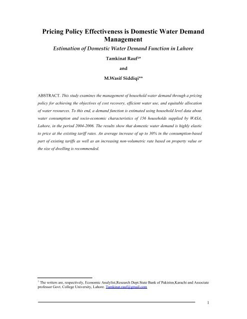
<strong>Pricing</strong> <strong>Policy</strong> <strong>Effectiveness</strong> <strong>is</strong> <strong>Domestic</strong> <strong>Water</strong> <strong>Demand</strong><br />
<strong>Management</strong><br />
Estimation of <strong>Domestic</strong> <strong>Water</strong> <strong>Demand</strong> Function in Lahore<br />
Tamkinat Rauf 1 *<br />
and<br />
M.Wasif Siddiqi**<br />
ABSTRACT. Th<strong>is</strong> study examines the management of household water demand through a pricing<br />
policy for achieving the objectives of cost recovery, efficient water use, and equitable allocation<br />
of water resources. To th<strong>is</strong> end, a demand function <strong>is</strong> estimated using household level data about<br />
water consumption and socio-economic character<strong>is</strong>tics of 156 households supplied by WASA,<br />
Lahore, in the period 2004-2006. The results show that domestic water demand <strong>is</strong> highly elastic<br />
to price at the ex<strong>is</strong>ting tariff rates. An average increase of up to 30% in the consumption-based<br />
part of ex<strong>is</strong>ting tariffs as well as an increasing non-volumetric rate based on property value or<br />
the size of dwelling <strong>is</strong> recommended.<br />
1 The writers are, respectively, Economic Analyl<strong>is</strong>t,Research Dept.State Bank of Pak<strong>is</strong>tsn,Karachi and Associate<br />
professor Govt. College University, Lahore. Tamkinat.rauf@gmail.com<br />
1
1. INTRODUCTION<br />
The population of Lahore has roughly doubled over the past twenty years, and an increase of<br />
two million <strong>is</strong> expected by the year 2020 (UN, 2005). Th<strong>is</strong> has important implications for city<br />
planning as demand for housing, electricity, water, sanitation, public health, education, and<br />
infrastructure grows accordingly.<br />
WASA, the city’s official water supplier, has often responded to the growing demand by<br />
offering the supply-side solution: augmenting supply capacity by exploiting new water resources. 2<br />
Such investments are costly, but in view of the public good nature of water, WASA has kept tariffs<br />
well below the cost-recovery level, relying on heavy loans and subsidies. While th<strong>is</strong> arrangement may<br />
have worked in the past, it <strong>is</strong> now becoming increasingly unsustainable, because 1) WASA <strong>is</strong> facing<br />
severe financial constraints and which has led to poor service and underinvestment, and 2) the<br />
environmental cost of extracting water <strong>is</strong> increasing.<br />
With its low tariff rates and continually increasing costs, the WASA Lahore <strong>is</strong> unable to meet<br />
even its O&M costs (WASA, 2007). WASA has been receiving financial ass<strong>is</strong>tance from the<br />
provincial and Lahore d<strong>is</strong>trict governments as well as international donors in the form of grants and<br />
loans with the grant element gradually dimin<strong>is</strong>hing over the passage of time. WASA currently owes<br />
Rs. 5.6 billion to these agencies and <strong>is</strong> in no position to make the repayment (WASA, 2007).<br />
Deteriorating financial situation has also led to short-term planning, reactive operational strategy, and<br />
underinvestment in asset maintenance, future capacity, IT equipment, management and accounting<br />
information system, and training (IFC, 2005). Consequently, WASA has shown suboptimal<br />
performance: low pressure and irregular supply, leakages, poor customer service, etc.<br />
Secondly, ind<strong>is</strong>criminate and unplanned exploitation of water resources may result in severe<br />
water shortages in future. <strong>Water</strong> supply in Lahore depends essentially on groundwater pumped<br />
through privately or publicly-owned tubewells and hand pumps. However, groundwater <strong>is</strong> a limited<br />
resource, recharged only once a year during the monsoon. Reportedly, the groundwater table has been<br />
falling. 3 Falling water tables increase the cost of pumping, as more energy <strong>is</strong> required to pump deep<br />
water. Furthermore, the International <strong>Water</strong> <strong>Management</strong> Institute has predicted severe water shortage<br />
in the country by the year 2025, that will threaten even the sustainability of agriculture (IWMI, 2000).<br />
2 In line with the demands of the growing population, WASA has continuously expanded its supply capacity in<br />
the past. Currently, WASA produces 350 million gallons of water per day with its 400 tubewells. Over 25 more<br />
tubewells have been approved under the 2007-08 budget of the agency (WASA, 2007).<br />
3 Over the year 2002-03, the groundwater table in Punjab fell on average by 0.61 percent (Govt. of the Punjab,<br />
2005). More recent estimates were not available.<br />
2
Relentless extraction of water may also lead to an irreversible decline in the ability of the region to<br />
store water in the ground (Gleick, 1998).<br />
<strong>Water</strong> produced by WASA <strong>is</strong> not being efficiently util<strong>is</strong>ed. The basic water requirement for<br />
drinking, sanitation, bathing, and food preparation <strong>is</strong> 13.2 gallons pcd, while WASA produces 80<br />
gallons pcd – an excess of over 66 gallons pcd (WASA, 2007). 4 Evidently, there <strong>is</strong> an excess demand<br />
– people demand more quantities of water than they would if they were made to pay the true<br />
environmental and supply cost of water. Clearly, the supply solution d<strong>is</strong>cussed earlier <strong>is</strong> not the best<br />
answer to the apparently growing demand.<br />
Instead, WASA should be looking at demand management that involves pricing policies and<br />
rationing – notionally allocating a fixed amount of water to each household, based upon lifeline and<br />
household size considerations. However, though rationing brings a definite change in demand, it <strong>is</strong><br />
difficult to implement and may not be widely acceptable. <strong>Pricing</strong> policies, on the other hand, have<br />
been successfully implemented in countries like Brazil, Canada, France, Spain, the United Kingdom,<br />
and the United States.<br />
Through pricing policies ex<strong>is</strong>ting demand patterns are modified to achieve various objectives,<br />
such as cost recovery, conservation, and equitable allocation of water among different income groups.<br />
To implement such a policy successfully, the value that consumers place on water must be known.<br />
Th<strong>is</strong> value <strong>is</strong> reflected by the price elasticity of water demand – the percentage change in demand that<br />
will be caused by a percentage change in price. If the demand <strong>is</strong> inelastic, it shows that at the ex<strong>is</strong>ting<br />
prices, the consumer highly values water and will be willing to pay a higher price in order to consume<br />
the same amount of water. On the other hand, if elasticity <strong>is</strong> high, the consumer indicates a<br />
willingness to reduce/increase the use of water with changes in its price. And if price <strong>is</strong> increased, he<br />
would shift a part of h<strong>is</strong> expenditures elsewhere. Clearly, th<strong>is</strong> information <strong>is</strong> fundamental in deciding<br />
the manner in which tariff should be structured.<br />
Another important aspect of a pricing policy <strong>is</strong> that households with different socio-economic<br />
settings, especially different income levels, will be affected differently, often giving r<strong>is</strong>e to <strong>is</strong>sues of<br />
equity – fairness in the d<strong>is</strong>tribution of cost and conservation burdens. How water demand varies<br />
across different types of household <strong>is</strong> central in estimating the implications of a pricing policy on<br />
equity.<br />
4 The internationally recommended lifeline supply <strong>is</strong> 50 litres pcd. 1 litre = 0.2642 gallons<br />
3
Th<strong>is</strong> study estimates household water demand in Lahore in order to explore the potential of a<br />
pricing policy to increase revenues and d<strong>is</strong>courage inefficient water use while ensuring a fair<br />
d<strong>is</strong>tribution of water in the community.<br />
The thes<strong>is</strong> <strong>is</strong> organ<strong>is</strong>ed as follows: Section two reviews literature on water demand. Section<br />
three gives a description of the study area. Th<strong>is</strong> <strong>is</strong> followed by the methodology: section four,<br />
sampling framework; section five, theoretical framework; and section six, data description. Results<br />
are presented in section seven, followed by policy recommendations in section eight, the last section.<br />
2. LITERATURE REVIEW<br />
The estimation of urban residential water demand has been an area of wide and growing<br />
interest world-wide for the past three decades. However, most of the ex<strong>is</strong>ting literature pertains to the<br />
developed world: the United States and Europe (Agthe and Billings, 1987, Arbues and Villanua,<br />
2006, Batchelor, 1975, Chicoine and Ramamurthy, 1986, Foster and Beattie, 1979, 1981, Hansen<br />
1996, Headley, 1963, Hewitt and Hanemann, 1995, Nauges and Thomas, 2000, Ne<strong>is</strong>wiadomy and<br />
Molina, 1989, 1991, Renwick and Archibald, 1998, Wong, 1972). So far, no comprehensive study has<br />
been conducted in Pak<strong>is</strong>tan to estimate the urban residential water demand and neither has the<br />
researcher come across any such study of similar-income countries. Therefore, the reviewed literature<br />
has limited usefulness in many aspects. What follows <strong>is</strong> an analytical review of the methodologies and<br />
data types used in previous studies and a brief assessment of the suitability of these methods in the<br />
present context.<br />
<strong>Water</strong> demand estimation studies have used various sorts of data: time-series (Agthe and<br />
Billings, 1987, Hansen, 1996), panel (Arbues and Villanua, 2006, Nauges and Thomas, 2000,<br />
Ne<strong>is</strong>wiadomy and Molina, 1989, 1991, Renwick and Archibald, 1998) and cross-sectional (Chicoine<br />
and Ramamurthy, 1986, Foster and Beattie, 1979, 1981, Headley, 1963, Wong, 1972). Time series<br />
data <strong>is</strong> useful to study the effects of a policy change such as restructuring of block-rates, rationing of<br />
water supply, or the introduction of a new water-related appliance. Time series data also captures the<br />
effect of weather. A drawback of such data <strong>is</strong> that it <strong>is</strong> aggregate: summing or averaging quantities,<br />
such as consumption, income, and prices, for the entire community. For th<strong>is</strong> reason, results derived<br />
from time series data have limited usefulness.<br />
Cross-sectional data on the other hand can be collected for d<strong>is</strong>aggregate units, such as<br />
individuals, households, or localities. Th<strong>is</strong> data holds more information than time-series data, and <strong>is</strong><br />
appropriate for estimating demand across different groups. However, cross-sectional units may have<br />
4
too much variability which can cause heteroscedasticity, in which case the OLS estimators have high<br />
variances. 5<br />
The most useful approach <strong>is</strong> perhaps the panel data, because it combines elements of both<br />
cross-sectional and time-series: more variables can be studied while time effect <strong>is</strong> also captured. Panel<br />
data also increases the number of observations, and hence the accuracy of the model. For these reason,<br />
th<strong>is</strong> study has used panel data.<br />
Urban water <strong>is</strong> usually priced under ‘block-rate’ schedules: a volume-based rate cons<strong>is</strong>ting of<br />
a sequence of marginal prices for different consumption blocks. <strong>Water</strong> use in each billing period <strong>is</strong><br />
divided into successive blocks with use in each ascending block charged at a different price. The<br />
block rate schedules can be progressive or regressive with increased consumption. The schedules are<br />
establ<strong>is</strong>hed to ensure efficient use of resource, as well as to achieve equity, environmental<br />
conservation, cost recovery, and public acceptability. An important point of contention in water<br />
demand studies has been the specification of the price variable in the model (Charney and Woodard,<br />
1984, Chicoine and Ramamurthy, 1986, Foster and Beattie, 1981, Opaluch 1982, 1984). <strong>Water</strong><br />
demand studies use two alternative types of price specifications:<br />
1. Marginal price of the block under which the consumer falls plus a ‘difference variable’ (following<br />
Taylor, 1975 and Nordin, 1976). The difference variable <strong>is</strong> calculated as the difference between what<br />
the consumer actually pays and what he would have been charged if all consumption units were<br />
charged at the marginal price of the last unit of consumption. The difference variable <strong>is</strong> used along<br />
with the marginal price.<br />
2. Average price – the total water expenditure by the consumer in a billing period divided by the total<br />
water consumed in that period.<br />
Proponents of the difference variable specification (Agthe and Billings, 1987, Renwick and<br />
Archibald, 1998) argue that the consumer <strong>is</strong> well-informed and therefore responds to the marginal<br />
price and difference variable. On the other hand, those who favour average pricing argue that the<br />
consumer does not devote time to studying the tariff structure and only has a rough idea of what he<br />
pays for h<strong>is</strong> consumption (Foster and Beattie, 1981).<br />
Nieswiadomy and Molina (1991) and Opaluch (1982) have suggested stat<strong>is</strong>tical tests to<br />
determine the price to which the consumers actually respond. The advantage of one test over the other<br />
5 Heteroscedasticity <strong>is</strong> defined as non-constant variances of residuals. In the presence of heteroscedasticity, OLS<br />
estimators remain unbiased and cons<strong>is</strong>tent but they no longer have minimum variance.<br />
5
was not readily apparent. Th<strong>is</strong> study has used the more recent Nieswiadomy and Molina (1991) price<br />
specification test to determine the correct price specification.<br />
It has been further argued that ill-informed consumers react to past rather than current prices<br />
(Charney and Woodard, 1984), and hence the appropriate specification of price would be the lagged<br />
(average) price. The lagged-price specification has not been used in the present study because the<br />
WASA tariff schedule <strong>is</strong> rather uncomplicated (only three blocks) and has been rev<strong>is</strong>ed only once<br />
since 1998. However, past bills may have some impact on the consumers’ dec<strong>is</strong>ion-making; a lagged<br />
consumption variable has therefore been added as a regressor.<br />
With multi-part block rates, prices are endogenously determined by the quantity demanded,<br />
and hence a the model <strong>is</strong> based on simultaneous equations. Under simultaneity, the OLS method<br />
yields biased and incons<strong>is</strong>tent estimates. Most water demand studies have used either instrumental<br />
variables (Nauges and Thomas, 2000, Ne<strong>is</strong>wiadomy and Molina, 1989, 1991) or two-stage least<br />
squares (Agthe and Billings, 1987, Renwick and Archibald, 1998) to remove the ‘simultaneity bias’.<br />
Arbues and Villanua (2006) have used a ‘dynamic panel model’ which <strong>is</strong> applicable to cases where<br />
the price <strong>is</strong> lagged to a degree such that it <strong>is</strong> no longer correlated with the error term in the current<br />
period. Hewitt and Hanemann (1995) have used a complex d<strong>is</strong>crete/continuous model that builds on<br />
the d<strong>is</strong>continuous nature of the budget constraint faced by the consumer under block-pricing. The<br />
OLS method has been used in studies where uniform rates were charged (Hansen, 1996) or the<br />
demand function was formulated under restrictive assumptions (Chicoine and Ramamurthy, 1986,<br />
Foster and Beattie, 1979, Headley, 1963, Wong, 1972). Th<strong>is</strong> study has used two-stage least squares<br />
method of estimation.<br />
Different functional forms have been used in domestic water demand studies, including linear<br />
(Agthe and Billings, 1987, Batchelor, 1975, Renwick and Archibald, 1998, Nauges and Thomas,<br />
2000, Ne<strong>is</strong>wiadomy and Molina, 1989), double-log (Foster and Beattie, 1979, 1981, Hewitt and<br />
Hanemann, 1995, Ne<strong>is</strong>wiadomy and Molina, 1991, Wong, 1972) and semi-log models (Hansen,<br />
1996). However, there <strong>is</strong> no evidence to indicate which <strong>is</strong> the most appropriate form. Linear models<br />
are easy to estimate while double-log models are useful because the coefficients give estimates of<br />
elasticities. Following Arbues and Villanua (2006), in order to establ<strong>is</strong>h the most adequate functional<br />
form, th<strong>is</strong> study has estimated all three types of specifications: linear, double-log, and semi-log. The<br />
most stat<strong>is</strong>tically and theoretically sound model has been selected for drawing conclusions.<br />
6
3. WATER SUPPLY IN LAHORE<br />
Lahore <strong>is</strong> one of the oldest cities of South Asia and <strong>is</strong> the provincial capital of Punjab. The<br />
Lahore d<strong>is</strong>trict spreads over an area of 1,772 square kilometres with a population density of over<br />
3,566 persons per thousand square kilometres (Govt. of the Punjab, 2005). Population-w<strong>is</strong>e, Lahore <strong>is</strong><br />
the second largest city in Pak<strong>is</strong>tan, fifth-largest in South Asia, and 23rd in the world (World<br />
Gazetteer, 2007). The current urban population <strong>is</strong> over 6.6 million and <strong>is</strong> expected to exceed eight<br />
million by the year 2020 (UN, 2004).<br />
The Lahore Development Authority (LDA) <strong>is</strong> the chief municipal body responsible for<br />
preparation and implementation of schemes for environmental improvements, housing, slum<br />
improvement, solid waste d<strong>is</strong>posal, transportation and traffic, health and education facilities, and<br />
water supply and sewerage in Lahore City area under the LDA Act, 1975. The chief water supplier in<br />
urban Lahore <strong>is</strong> WASA, formed under the Act.<br />
The WASA service area extends to 350 square kilometres, supplying water and sewerage<br />
services to a population of over five million (IFC, 2005). Other private water suppliers also ex<strong>is</strong>t in<br />
Lahore City, but there <strong>is</strong> no official record of their number and coverage. For admin<strong>is</strong>trative purposes,<br />
the area covered by WASA <strong>is</strong> divided into six blocks called ‘towns’: Allama Iqbal Town, Aziz Bhatti<br />
Town, Ravi Town, Shalimar Town, Ganj Baksh Town, and N<strong>is</strong>htar Town. Each town <strong>is</strong> further<br />
divided into O&M sub-div<strong>is</strong>ions.<br />
Though located along the bank of River Ravi, water supply in Lahore depends on<br />
groundwater, the river being the most polluted in the entire country. 6 For Lahore, groundwater <strong>is</strong> an<br />
ideal source of water because it <strong>is</strong> relatively free of impurities and therefore little or no treatment of<br />
the water <strong>is</strong> needed before it <strong>is</strong> put to household use.<br />
Table 3.1: WASA Admin<strong>is</strong>trative Div<strong>is</strong>ion<br />
Town<br />
Allama Iqbal Town<br />
Aziz Bhatti Town<br />
Ganj Baksh Town<br />
O&M Sub-div<strong>is</strong>ions<br />
Allama Iqbal Town, Samanabad, Johar Town, Ichhra<br />
Taj Pura, Mustafabad<br />
Ravi Road, Kr<strong>is</strong>han Nagar, Shimla Hill, Mozang, Gulberg<br />
6 River Ravi <strong>is</strong> the most polluted river in Pak<strong>is</strong>tan, receiving 47 percent of the total municipal and industrial<br />
pollution d<strong>is</strong>charged into all rivers in the country. According to the World Wildlife Fund, extreme pollution has<br />
destroyed around 42 f<strong>is</strong>h species that the river was home to. Even contact with the river water has been reported<br />
to cause severe skin d<strong>is</strong>eases. The water <strong>is</strong> certainly unfit for drinking. (EDC News:<br />
http://www.edcnews.se/Cases/PakRaviriver.html)<br />
7
N<strong>is</strong>htar Town<br />
Ravi Town<br />
Shalimar Town<br />
Green Town, Industrial Area, Township, Garden Town<br />
Shahdara, Data Nagar, City, Farkhabad, M<strong>is</strong>ri Shah,<br />
Shadbagh<br />
Baghbanpura, Mughalpura<br />
<strong>Water</strong> <strong>Pricing</strong> under WASA<br />
WASA water tariffs are apparently based on cost-considerations, but are well below the cost<br />
recovery level. The objective <strong>is</strong> seemingly to recover an acceptable portion of the cost rather than the<br />
full costs, that being a compulsion due to political considerations. 7<br />
Table 3.2: ARV-based Billing Structure for <strong>Domestic</strong> Unmetered Connections<br />
ARV (Rs.)<br />
Rate (Rs. per month)<br />
January 1998 May 2004<br />
Up to 400 70.55 98.77<br />
401-500 108.80 152.32<br />
501-720 185.30 259.42<br />
721-1000 323.00 452.20<br />
10001-1500 455.00 637.84<br />
1501-2388 479.40 671.16<br />
2389-4370 510.00 714.00<br />
4371-4499 533.00 747.32<br />
4500 and above 84% of ARV 84% of ARV<br />
Table 3.3: <strong>Water</strong> Tariff Structure for <strong>Domestic</strong> Metered Connections<br />
Consumption (gallons)<br />
Rate (Rs. per 1,000 gallons per month)<br />
January 1998 May 2004<br />
Up to 5,000 9.20 12.88<br />
5,001-20,000 14.90 20.86<br />
20,001 and above 19.50 27.30<br />
Source: WASA, Lahore.<br />
7 The City D<strong>is</strong>trict Govt. has not allowed WASA to ra<strong>is</strong>e tariffs for the past three years in spite a 10 percent<br />
increase in the electricity rates (WASA, 2007).<br />
8
Tariffs for both metered and unmetered connections have been rev<strong>is</strong>ed thrice over the past<br />
decade: in July 1997, in January 1998, and then in May 2004. No annual inflation adjustments are<br />
made.<br />
<strong>Water</strong> <strong>is</strong> charged volumetrically where the connection <strong>is</strong> metered, while unmetered<br />
connections are charged on the bas<strong>is</strong> of the annual rental value (ARV) of the house. 8 The ARV <strong>is</strong><br />
divided into nine bands ranging from Rs.400 to Rs.4, 500 and above. However, since ARV-based<br />
charges do not directly affect consumption, we have selected only metered households for th<strong>is</strong> study.<br />
Currently only 30 percent of WASA connections are metered but WASA <strong>is</strong> making<br />
substantial efforts to meter all ex<strong>is</strong>ting connections (WASA, 2007). 9 No new unmetered connections<br />
have been <strong>is</strong>sued since January 1997. Metered connections are charged with a two-part tariff: a<br />
variable volume-based part and a fixed part. The fixed part includes monthly connection fee of Rs.12<br />
plus a flat charge of Rs.3 per month. The volume-based charges are divided into three ascending<br />
volumetric blocks, that <strong>is</strong>, consumption in each succeeding block <strong>is</strong> charged higher than the previous<br />
block.<br />
4. A MODEL FOR WATER DEMAND<br />
The domestic demand for water ar<strong>is</strong>es from its use for sanitation, bathing, washing clothes,<br />
cleaning homes and cars, cooking and drinking, watering lawns, cooling, and recreational activities.<br />
Like other commodities, the demand for water <strong>is</strong> expected to fall with price and increase with income.<br />
Some other factors, such as the prices of water-related appliances, household size, house size, and<br />
weather, etc. are also expected to have some influence on water demand. Based on these<br />
considerations, a model for domestic water demand <strong>is</strong> presented below.<br />
As d<strong>is</strong>cussed in chapter two, the price effect under block-rate pricing enters the demand<br />
equation indirectly. If consumers are well-informed of the price structure, they respond to the<br />
marginal price (MP), that <strong>is</strong>, the price of their final consumption block. But fully informed consumers<br />
are also aware of the benefit that they gain by having paid less on the initial blocks. Th<strong>is</strong> benefit<br />
enters the demand equation as the ‘difference variable’ – the difference between what the consumers<br />
actually pay and what they would have paid had all units been priced at the marginal price. The<br />
difference variable (DV) <strong>is</strong> computed as follows:<br />
8 Annual Rental Value (ARV) <strong>is</strong> defined as the gross annual rent at which a land or a building might be expected<br />
to be let from year to year, less deductions for repair and maintenance. (World Bank and The Urban Unit,<br />
Lahore, 2006.)<br />
9 WASA allocated Rs.29 million for the procurement of domestic water meters in 2007-08. (WASA budget<br />
document, 2007.)<br />
9
DV = [P1Q1 + P2Q2 + P3 (Q-Q1-Q2)] – [P3Q] [1]<br />
Where P1, P2, and P3 are the respective prices charged under the successive blocks. Q1 and Q2 are<br />
the respective consumption limits for the first two blocks.<br />
Alternatively, if the consumers are not fully aware of the water charges, they approximate the<br />
average price of water by dividing the total water expenditure in a billing period by the quantity of<br />
water consumed in that period. The average price (AP) <strong>is</strong> computed as:<br />
AP = [P1Q1 + P2Q2 + P3 (Q-Q1-Q2)] / Q [2]<br />
The correct specification of price <strong>is</strong> largely a circumstantial question. For example, in<br />
Zaragoza, Spain, where the tariff rate cons<strong>is</strong>ts of 205 consumption blocks, it <strong>is</strong> reasonable to assume<br />
that consumers cannot be fully aware of such a complex tariff structure, and therefore AP<br />
specification can be used. 10 In the present case there are only three blocks and, analogously, it can be<br />
argued that the marginal price specification <strong>is</strong> correct. However, a more rigorous approach can also be<br />
adopted.<br />
Under increasing block rates, the perceived price (P*) must lie somewhere between the<br />
average and marginal prices. Let ‘k’ be a parameter that measures price perception. We may write,<br />
P* = MP (AP/MP) k<br />
The value of ‘k’ will lie somewhere between zero and one. If ‘k’ <strong>is</strong> found to be zero, then MP <strong>is</strong> the<br />
perceived price. If it <strong>is</strong> equal to one, the perceived price <strong>is</strong> AP. If neither of these cases holds, then the<br />
perceived price lies between AP and MP.<br />
To test the value of ‘k’, the following equation <strong>is</strong> estimated:<br />
lnQ = a 0 + a 1 lnMP + a 1 kln(AP/MP)+ ΣaiXi + µ [3]<br />
Where Xi denotes predetermined variables.<br />
Standard t-test can be applied to test the value of ‘k’.<br />
Household water use <strong>is</strong> expected to increase with increase in income. More affluent<br />
households are likely to use water less vigilantly than low income households. They are also more<br />
likely to use water for washing cars, watering lawns, and swimming pools. A strong relationship has<br />
also been found between use of water-based appliances and household water demand (Batchelor,<br />
1975). However, reliable data of these indicators can be difficult to obtain. Therefore, information<br />
10 Arbues, Fernando and Villanua Inmaculada (2006). Potential for <strong>Pricing</strong> Policies in <strong>Water</strong> Resource<br />
<strong>Management</strong>: Estimation of Urban Residential <strong>Water</strong> <strong>Demand</strong> in Zaragoza, Spain.<br />
10
about the house value was used as an indicator of wealth, a proxy for income, hoping that it would<br />
also take into account some of the other water-related variables. 11<br />
The size of the dwelling and the number of residents <strong>is</strong> also expected to influence water use.<br />
Larger houses use more water for cleaning and irrigation of lawns, thus water use should increase<br />
with the house size. The relationship of demand with the number of residents <strong>is</strong>, however, not so<br />
direct. Generally, high income families are smaller than low income families. Per capita water<br />
consumption may, therefore, be lower in low income families, in which case there may be a negative<br />
effect of household size on consumption.<br />
Three water-related activities are predominantly influenced by weather: watering lawns, using<br />
room-coolers, and bathing. As temperatures r<strong>is</strong>e, these activities become more frequent. A weather<br />
variable has been included in the demand model to capture th<strong>is</strong> effect.<br />
Past bills, and therefore consumption patterns, are likely to have some influence a consumer’s<br />
dec<strong>is</strong>ion-making in the future. Moreover, th<strong>is</strong> effect <strong>is</strong> likely to decline with time: older bills wielding<br />
lesser influence than the ones that follow. In such a situation, Koyck (1954) has proposed substituting<br />
the lagged explanatory variables by one single lagged dependent variable that appears among the<br />
regressors. 12 Following th<strong>is</strong> proposition, a lagged consumption term has been included. The<br />
coefficient of th<strong>is</strong> variable must be positive and must not exceed one.<br />
<strong>Domestic</strong> water-meters are owned by either WASA or the consumers. Entitlement to the<br />
meter does not directly influence demand but it may influence the quality and accuracy of the meter:<br />
if the meter overestimates consumption, the consumer would make sure that the fault <strong>is</strong> fixed. If, on<br />
the other hand, WASA meters under-read consumption, WASA will ensure accuracy. A dummy<br />
variable has been used to capture th<strong>is</strong> affect. The dummy takes a unit value if meter <strong>is</strong> owned by<br />
consumer, and a zero value if owned by WASA. Possibly, th<strong>is</strong> dummy will be negatively related with<br />
the recorded consumption.<br />
Fixed Effects<br />
As d<strong>is</strong>cussed above, many factors cause variability in demand patterns across households:<br />
household income, per capita income, ages of residents, lawn size, car ownership, and use of waterrelated<br />
appliances. However, not all these variable could be included in the demand model. The effect<br />
of m<strong>is</strong>sing variables <strong>is</strong> reflected in the intercept term.<br />
11 Following Batchelor (1975), and Nieswiadomy and Molina (1989, 1991).<br />
12 See: Koutsoyiann<strong>is</strong>, A. (1972). Theory of Econometrics (2 nd ed.). pp.304-6.<br />
11
When m<strong>is</strong>sing variables differ significantly across areas or communities, th<strong>is</strong> may give r<strong>is</strong>e to<br />
a ‘differential intercept model’ – a model in which the regression line has varying intercepts for<br />
different population groups. To estimate these differences across groups, a ‘fixed effects model’ <strong>is</strong><br />
used, based upon dummy variables assigned on the bas<strong>is</strong> of geographical location. 13 Five intercept<br />
dummies have been introduced for Aziz Bhatti, Allama Iqbal, Ganj Baksh, Ravi, and Shalimar towns.<br />
N<strong>is</strong>htar town <strong>is</strong> the benchmark category.<br />
Table 4.1: Notation and Variable Description<br />
Variable Indicator<br />
Qt<br />
AP<br />
MP<br />
DV<br />
W<br />
NR<br />
L<br />
T<br />
Dmo<br />
Dait<br />
Dabt<br />
Dgbt<br />
Drt<br />
Dst<br />
Description<br />
Quantity of water consumed in billing period t<br />
Average price<br />
Marginal price<br />
Difference variable<br />
Wealth<br />
Number of residents<br />
Plot size<br />
Average temperature in period t<br />
Meter ownership dummy<br />
Dummy for residence in Allama Iqbal Town<br />
Dummy for residence in Aziz Bhatti Town<br />
Dummy for residence in Ganj Baksh Town<br />
Dummy for residence in Ravi Town<br />
Dummy for residence in Shalimar Town<br />
Functional Form<br />
As d<strong>is</strong>cussed in chapter two, there <strong>is</strong> no theoretical bas<strong>is</strong> for adopting any specific functional<br />
form. Past studies have typically used linear, semi-log, and double-log forms.<br />
The MacKinnon, White, and Davidson test (MWD test) was used to choose between linear<br />
and double-log forms. The results recommend a double-log functional form. However, there were no<br />
a priori grounds for choosing between semi-log and double-log functions, and therefore, both<br />
functions were estimated. Double-log models have the advantage that their estimators give the<br />
13 Fixed Effect Model (FEM): A model in which the intercept term varies over sampling units but <strong>is</strong> constant<br />
over time.<br />
12
elasticities of the variables, thus simplifying interpretation. Semi-log models are useful to estimate<br />
elasticity across different population groups, as the coefficients give ‘semi-elasticity’: elasticity of the<br />
dependent variable with respect to varying values of the regressors.<br />
The Estimated Models<br />
The following demand models were estimated:<br />
1. MP Models<br />
DV = [P 1 Q 1 + P 2 Q 2 + P 3 (Q – Q 1 – Q 2 )] – P 3 Q [1]<br />
Semi-log:<br />
lnQ = β 0 + β 1 MP + β 2 T + β 3 W + β 4 NR + β 5 L + β 6 Dmo + β 7 Dabt + β 8 Dait + β 9 Dgbt + β 10 Drt + β 11 Dst<br />
+ β 12 DVµ 3 [3]<br />
Double-log:<br />
lnQ = β 0 + β 1 lnAP + β 2 lnT + β 3 lnW + β 4 lnNR + β 5 lnL + β 6 Dmo + β 7 Dabt + β 8 Dait + β 9 Dgbt + β 10 Drt<br />
+ β 11 Dst + β 11 D β 11 DV + µ 2 [4]<br />
2. AP Models<br />
AP = [P 1 Q 1 + P 2 Q 2 + P 3 (Q – Q 1 – Q 2 )] / Q [2]<br />
Semi-log:<br />
lnQ = β 0 + β 1 AP + β 2 T + β 3 W + β 4 NR + β 5 L + β 6 Dmo + β 7 Dabt + β 8 Dait + β 9 Dgbt + β 10 Drt + β 11 Dst +<br />
µ 3 [5]<br />
Double-log:<br />
lnQ = β 0 + β 1 lnAP + β 2 lnT + β 3 lnW + β 4 lnNR + β 5 lnL + β 6 Dmo + β 7 Dabt + β 8 Dait + β 9 Dgbt + β 10 Drt<br />
+ β 11 Dst + µ 2 [6]<br />
Estimation Technique<br />
Since price <strong>is</strong> endogenously determined by the model a ‘simultaneous equation bias’ <strong>is</strong> likely<br />
to ar<strong>is</strong>e. 14 Hausman test was used to check for if the simultaneity problem ex<strong>is</strong>ted. The results showed<br />
that both price variables, as well as the difference variable created a simultaneous equation bias under<br />
OLS.<br />
14 Simultaneous equations bias: Incons<strong>is</strong>tency of OLS estimators in a simultaneous equations system.<br />
13
The 2SLS technique was used to eliminate th<strong>is</strong> bias. In the first stage, instrumental variables<br />
were created for all the three variables, by separately regressing them on all pre-determined variables<br />
as well as the three block prices. In the second stage, OLS was used to estimate equations 3, 4, 5, and<br />
6, replacing AP, MP, and DV by their respective instrumental variables.<br />
5. DATA DESCRIPTION<br />
Three sets of information were collected: household level data about consumption and<br />
household character<strong>is</strong>tics, tariff structures, and weather.<br />
Household-level information: Primary data for the study was obtained from WASA, Lahore. The data<br />
set contained the following information about 156 households:<br />
Location: Information about the town in which the connection <strong>is</strong> located.<br />
Consumption: <strong>Water</strong> consumption in gallons from January 2004 to December 2006. Meter reading <strong>is</strong><br />
carried out by WASA with a back-lag of two months: that <strong>is</strong>, for the billing cycle March-April, the<br />
meter <strong>is</strong> read in the last week of February. For the subsequent cycle, May-June, the meter <strong>is</strong> read in<br />
the last week of April. In th<strong>is</strong> way, the March-April bill <strong>is</strong> based on January-February consumption,<br />
and May-June bill <strong>is</strong> based on March-April consumption.<br />
The variable used in th<strong>is</strong> study <strong>is</strong> the consumption during the billing period, the previous<br />
month’s meter-reading, rather than the meter-reading recorded in the billing period. Eighteen meter<br />
readings were recorded per household.<br />
Plot size: The plot size in marlas.<br />
Property Value: Property value in Rupees.<br />
Number of Residents: The number of residents living in a house.<br />
Meter-ownership: Information about whether the meter <strong>is</strong> owned by WASA or the consumer.<br />
Tariff Structure: The tariff structures for domestic metered connections since January 2004 were<br />
provided by WASA.<br />
Table 6.1: Descriptive Stat<strong>is</strong>tics<br />
Variable Mean Std. Deviation Minimum Maximum<br />
Consumption (1,000 gallons<br />
per billing period)<br />
17.9 14.9 2.00 155.12<br />
Average Price (Rs.) 17.7 2.4 9.2 26.0<br />
Marginal PriceP (Rs.) 21.8 3.5 9.2 27.3<br />
14
Household Size 6.3 1.8 2.0 11.0<br />
Plot Size (marlas) 8.7 13.9 1 160<br />
Property Value (Rs. lacs) 29.4 35.5 2.0 250.0<br />
<strong>Water</strong> Expenditure (Rs) 340.1 373.6 18.4 4033.9<br />
Temperature (Celsius) 30.4 6.2 18.5 38.6<br />
Weather: Information about the weather in Lahore was provided by the Pak<strong>is</strong>tan Meteorological<br />
Department. The data-set contained the maximum average monthly temperature recorded in degree<br />
Celsius from January 2004 to December 2006. The temperature values were averaged over two-month<br />
periods in line with WASA billing cycles.<br />
6. RESULTS<br />
The estimated demand model explains 60 percent of the variation in water consumption and <strong>is</strong><br />
stat<strong>is</strong>tically significant. 15 Price, plot size, household size, meter ownership, past water consumption,<br />
and the difference variable that captures the income effect have been found to significantly influence<br />
the household demand for water. The effect of weather <strong>is</strong> moderate while that of wealth, as measured<br />
by property value, <strong>is</strong> negligible.<br />
Whether water demand <strong>is</strong> more responsive to marginal or average price could not be<br />
establ<strong>is</strong>hed from the data. Therefore, both AP and MP models were estimated. The AP models<br />
showed a significant positive price-demand relationship, which <strong>is</strong> contrary to economic theory. Such<br />
contradiction <strong>is</strong> often attributed to stat<strong>is</strong>tical errors, such as multicollinearity or weak instrumental<br />
variables. However, no such error could be identified. Regardless of the reason for the d<strong>is</strong>crepancy,<br />
the AP models were not suited for drawing inferences. All following d<strong>is</strong>cussions and conclusions are<br />
based on MP models.<br />
The results show that the marginal price of water has a significant impact on water use: a<br />
percentage increase in the marginal price brings a 2.33 percent decline in average water use. A 10<br />
percent increase in the marginal price will bring down average water consumption by 23 percent.<br />
Table 7.1: Model Summary<br />
Stat<strong>is</strong>tic<br />
Value<br />
15 Though th<strong>is</strong> R 2 value <strong>is</strong> not very high, it <strong>is</strong> acceptable for panel data models with a large cross-sectional<br />
element. Cross-sectional data has high variance due to the diversity of the sampling units, and it <strong>is</strong> therefore<br />
difficult to fit a regression line that explains all the variation.<br />
15
R 2 0.600<br />
F-Stat<strong>is</strong>tic 304.163*<br />
Variable Coefficient t-ratio<br />
Intercept 0.54 (1.725)**<br />
Meter-ownership (Dummy) -0.06 (-2.180)*<br />
Difference Variable 2.89 (8.292)*<br />
Plot Size 0.04 (3.297)*<br />
Marginal Price -2.33 (-5.473)*<br />
Household Size -0.14 (-4.380)*<br />
Lagged Consumption 0.38 (10.402)*<br />
Temperature 0.05 (1.457)***<br />
Property Value -0.01 (-1.066)<br />
Location Dummies<br />
Aziz Bhatti Town -0.064 (-2.510)*<br />
Allama Iqbal Town -0.128 (-3.901)*<br />
Ganj Baksh Town 0.023 (0.942)<br />
Ravi Town -0.070 (-2.751)*<br />
Shalimar Town 0.010 (0.442)<br />
* = significant at 5% level.<br />
** = significant at 10% level.<br />
*** = significant at 15% level.<br />
The size of the plot, which presumably affects water use because of higher cleaning and lawn<br />
watering requirements, has a small but significant impact on domestic water use. For every percentage<br />
increase in the size of the plot, water consumption goes up by 0.041 percent. However, th<strong>is</strong><br />
information does not tell us about the individual impact of lawn size and house size and water use<br />
separately attributed to each variable. Possibly, water demand for one of the purposes may be more<br />
elastic than the other.<br />
The relationship of water demand and the number of residents living in a household was<br />
found negative, contrary to what was expected. As household size increases by one percent,<br />
consumption falls by 0.14 percent. Apparently small, th<strong>is</strong> connection <strong>is</strong> stat<strong>is</strong>tically significant and<br />
also has important implications for policymaking.<br />
Commonly, low income families are larger as compared to high income families. If large<br />
families consume less than small families, then there must be some underlying income connection.<br />
16
We may infer that low-income households consume less water per capita. However, more information<br />
<strong>is</strong> needed to substantiate th<strong>is</strong> inference.<br />
The difference variable has an effect of increasing demand by 2.89 percent with every<br />
percentage increase. In essence, the difference variable reflects the apparent increase in income from<br />
having paid less for some units of a commodity under increasing block rates – what <strong>is</strong> known in<br />
microeconomic theory as the ‘income effect’. As expected, th<strong>is</strong> income effect <strong>is</strong> positive. 16 Th<strong>is</strong><br />
means that as more d<strong>is</strong>criminatory tariffs are charged for consumption in successive blocks, the<br />
income effect induces consumers to increase water expenditure. However, as a policy variable, DV<br />
has limited value as it cannot be directly manipulated.<br />
Weather has a modest influence on domestic water consumption. A one percent r<strong>is</strong>e in<br />
temperature increases water demand by 0.05 percent. Th<strong>is</strong> means that water demand <strong>is</strong> higher in<br />
summer than in winter. 17<br />
The intercept term reflects the average water consumption for N<strong>is</strong>htar Town when all other<br />
variables are set to zero <strong>is</strong> 860.6 gallons per household per month if the meter <strong>is</strong> owned by WASA<br />
and 813.7 gallons if the meter <strong>is</strong> owned by the consumer. That means on average meter-ownership<br />
reduces water consumption by 46 gallons per month.<br />
According to the model, average household consumption of N<strong>is</strong>htar Towm <strong>is</strong> stat<strong>is</strong>tically<br />
similar to that of Ganj Baksh and Shalimar towns. Consumption in Aziz Bhatti and Ravi towns differ<br />
from N<strong>is</strong>htar Town by about 50 gallons per month, while Allama Iqbal Town households consume<br />
around 100 gallons less water than households in N<strong>is</strong>htar Town.<br />
7. POLICY RECOMMENDATIONS<br />
The results of th<strong>is</strong> study show that there <strong>is</strong> considerable potential to use demand management<br />
pricing policies. Therefore, a calculated re-arrangement of the tariff structure can be instrumental in<br />
encouraging efficient use of water, improving revenues, and ensuring universal lifeline supply.<br />
Conservation: Tariffs can be effectively used to induce efficient water use. At the current rate,<br />
household water use <strong>is</strong> extremely elastic to changes in prices. A small ten percent increase in the<br />
overall tariffs will cause an average household to conserve 2,000 gallons of water per month. A 30<br />
16 Note that the difference variable was originally negative. Natural log of the absolute values was included in<br />
the computations. However, the positive relationship of the variable consumption was also found in linear and<br />
log-linear models (See Appendix). We have therefore interpreted the coefficient as positive.<br />
17 The weather coefficient was significant at 15 percent level. If one adheres to the conventional five percent<br />
level, then the coefficient <strong>is</strong> stat<strong>is</strong>tically zero.<br />
17
percent increase will bring down water use to 2,700 gallons – close to the level of lifeline<br />
consumption. (See table 8.1). 18<br />
A drawback of these computations <strong>is</strong> that they are based on average consumption patterns,<br />
and do not give any indication of how the tariff increase will affect households with varying<br />
socioeconomic settings, particularly income levels. Taking into account these considerations may<br />
make an overall equal increase in tariffs undesirable.<br />
If an overall increase <strong>is</strong> not desirable, effective conservation can still be achieved by<br />
increasing the tariff of the final block – monthly consumption of over 20,000 gallons. Currently,<br />
average consumption in th<strong>is</strong> block <strong>is</strong> over 1,800 gallons. A 30 percent increase in the price of th<strong>is</strong><br />
block will induce average households to cut down over 1,000 gallons of monthly consumption. A<br />
larger increase can virtually eliminate per household water consumption beyond 20,000 gallons. (See<br />
table 8.2)<br />
Table 8.1: Impact of Price Increase on Monthly <strong>Water</strong> Use<br />
Current<br />
Tariff Increase<br />
10% 20% 30%<br />
Avg. MP (Rs.) 21.8 23.98 26.16 28.34<br />
Avg. Monthly Use (gallons) 8,900 6,900 4,800 2,700<br />
Table 8.2: Impact of Price Increase on <strong>Water</strong> Use in Block 3<br />
Current<br />
Tariff Increase<br />
30% 40% 50%<br />
Block 3 Price (Rs.) 27.30 35.49 38.22 40.95<br />
Avg. Monthly Use in Block 3<br />
(gallons)<br />
1,820 545 125 -300<br />
Cost Recovery: Typically, a tariff structure that <strong>is</strong> meant for budget balancing cons<strong>is</strong>ts of a large fixed<br />
part coupled with declining block rates (Montginoul, 2006). Declining block rates promote<br />
consumption leading to higher revenues and faster cost recovery on investments, while the fixed part<br />
increases the certainty of revenue projections.<br />
Though leading to immediate cost recovery, decreasing block rates are not compatible with<br />
promoting efficient water use, and assuming that conservation <strong>is</strong> more important of the two<br />
objectives, declining blocks rate are not adv<strong>is</strong>ed. Moreover, though increasing block rates do not<br />
18 Daily per capita lifeline <strong>is</strong> 13.21 gallons. The average household size <strong>is</strong> taken to be 7 (see Chapter 6 for<br />
descriptive stat<strong>is</strong>tics on household size). Lifeline water supply <strong>is</strong> calculated as: 13.21*7*30= 2,800 gpm.<br />
18
generate equally high revenue, they do lead to a cut-down in O&M costs while at the same time<br />
easing the need for new investments to increase supply capacity. Therefore, the management will not<br />
be ill-adv<strong>is</strong>ed to continue following increasing block rates.<br />
The non-volumetric part can also be effectively used to increase revenues. Currently the<br />
monthly non-volumetric charge cons<strong>is</strong>ts of a connection fee of Rs.3 and meter charge of Rs.12, that<br />
<strong>is</strong>, all households ind<strong>is</strong>criminately pay fixed charges of Rs.15 per month. The connection fee can be<br />
increased, uniformly or d<strong>is</strong>criminately, varying increasingly with the household’s ability to pay. The<br />
best measure of ability-to-pay <strong>is</strong> household income, but it <strong>is</strong> difficult to oblige people to provide<br />
correct information about their incomes. Alternatively, non-volumetric charges can be based on<br />
property value, ARV, or plot size.<br />
Allocation: The effect of a pricing policy may not be uniformly felt across all income groups. Past<br />
studies have found that ind<strong>is</strong>criminate tariff increase causes greater reduction in water use in lower<br />
income households than in higher income households (Agthe and Billings, 1987, Renwick and<br />
Archibald, 1998). If th<strong>is</strong> d<strong>is</strong>parity gets large enough, it can threaten the lifeline supply of vulnerable<br />
households.<br />
As a rule, water expenditure should not exceed five percent of the household income (WASA,<br />
2005). The lifeline water requirement for a seven-member household (2, 800 gallons per month) costs<br />
Rs.36.06. If the monthly income <strong>is</strong> Rs.5, 000, th<strong>is</strong> expenditure amounts to a bare 0.72 percent. If the<br />
tariff in the first block <strong>is</strong> increased by 50 percent, the lifeline consumption cost will amount to only<br />
1.1 percent of the expenditures of a household with above-mentioned features.<br />
Table#: Impact of Block 1 Price Increase on Lifeline Consumption<br />
Current<br />
Tariff Increase<br />
10% 20% 50%<br />
Price in Block 1 (Rs.) 12.88 14.17 15.46 19.32<br />
Cost of Avg. Household Lifeline<br />
Supply (Rs.)<br />
36.06 39.68 43.29 54.10<br />
Summing the d<strong>is</strong>cussion on pricing policies, one can see that there <strong>is</strong> significant room for<br />
increasing tariffs to achieve conservation and cost recovery objectives without r<strong>is</strong>king lifeline supply.<br />
19
APPENDIX<br />
I. Sampling Framework<br />
The sampling frame cons<strong>is</strong>ts of all domestic households that were metered prior to the beginning of the<br />
study period, i.e., January 2004. The correct number of such households was not available, but an estimate was<br />
made using the available information. Currently, WASA provides 480,000 domestic water connections of which<br />
only 30 percent are metered. Therefore, the sampling frame compr<strong>is</strong>es of 144,000 sampling units.<br />
Sample Size: WASA Lahore covers 90 percent of the households under its official jur<strong>is</strong>diction while the<br />
remaining 10 percent being provided by other (private) sources (WASA, 2007). In a randomly selected sample,<br />
the probability of a household having a WASA connection <strong>is</strong>, therefore, 90 percent. The sample size (n) was<br />
computed in the following way:<br />
n = PQ/SE(P) = 150<br />
where P <strong>is</strong> the percentage of households having a WASA connection and Q the percentage of households<br />
provided by others. If a six percent standard error <strong>is</strong> acceptable, a sample of 150 households <strong>is</strong> likely to contain<br />
90 percent households with a WASA connection. For th<strong>is</strong> study, the sample size was increased to 156<br />
households in order to achieve a better allocation of sampling units.<br />
Allocation of Sampling Units: The sampling frame was stratified on the bas<strong>is</strong> of WASA’s admin<strong>is</strong>trative<br />
div<strong>is</strong>ion. As d<strong>is</strong>cussed earlier, the WASA area <strong>is</strong> divided into six towns which are further divided into O&M<br />
units. Information about the exact population of these div<strong>is</strong>ions was not available; therefore sampling units were<br />
allocated proportionately according to a rough estimate of the population density under each subdiv<strong>is</strong>ion.<br />
Finally, the units were selected randomly using a random number table.<br />
Time Frame: It was intended that the time frame should include at least one tariff change, in order to better<br />
capture the effect of price on consumption. However, as mentioned earlier, tariffs have remained unchanged<br />
since May 2004. Before that, tariffs were last increased in January 1998. In order to include both (or more) tariff<br />
changes, the initial timing would have to be set at (or before) 1998. However, it was not practical to stretch the<br />
study period that long.<br />
As we go back in time, the number of metered connections, and hence the sampling frame, becomes<br />
smaller. Moreover, socio-economic and demographic character<strong>is</strong>tics, such as household size and income, would<br />
have significantly changed for each sampling unit over such a long time frame. Variations in these variables are<br />
difficult to measure and would have created considerable errors in the data.<br />
Because of these considerations, the time frame of the study was limited to the last three years, 2004 to<br />
2006, to include one tariff change while allowing for cons<strong>is</strong>tency of socioeconomic and demographic variables<br />
of each unit over th<strong>is</strong> period.<br />
20
Table 5.1: Allocation of Sampling Units<br />
Town Sampling Units O&M Sub-div<strong>is</strong>ion Sampling Units<br />
Allama Iqbal Town 25<br />
Allama Iqbal Town 5<br />
Ichhra 5<br />
Johar Town 5<br />
Sabzazar 5<br />
Samanabad 5<br />
Aziz Bhatti Town 25<br />
Taj Pura 13<br />
Mustafabad 12<br />
Ganj Baksh Town 25<br />
Gulberg 5<br />
Kr<strong>is</strong>han Nagar 5<br />
Mozang 5<br />
Ravi Road 5<br />
Shimla Hill 5<br />
N<strong>is</strong>htar Town 26<br />
Garden Town 6<br />
Green Town 6<br />
Industrial Area 7<br />
Township 7<br />
Ravi Town 44 30<br />
City 5<br />
Data Nagar 5<br />
Farkhabad 5<br />
M<strong>is</strong>ri Shah 5<br />
Shadbagh 5<br />
Shahdara 5<br />
Shalimar Town 25<br />
Baghbanpura 13<br />
Mughalpura 12<br />
Total 156 156<br />
II. Hausman Test<br />
Ho: Coefficient of residuals <strong>is</strong> stat<strong>is</strong>tically zero; no simultaneity problem<br />
H1: Coefficient of residuals <strong>is</strong> not stat<strong>is</strong>tically zero; simultaneity problem ex<strong>is</strong>ts<br />
Level of Significance: α = 0.05<br />
Test Stat<strong>is</strong>tic: t-ratio<br />
Computations and Conclusions:<br />
21
Variable<br />
Regression 1 Regression 2<br />
Residual<br />
Conclusion<br />
Dependent Independent Dependent Independent<br />
Coefficient<br />
1. AP AP Q_lag, P3, Dst, T,<br />
Q<br />
RES, PRE, T, Dabt,<br />
5.953<br />
Reject Ho.<br />
W, Dmo, Drt, L,<br />
Dmo, Dgbt, NR, L,<br />
(76.009)<br />
Conclude that<br />
Dabt, NR, Dgbt,<br />
Dst, Dait, W, Q_lag,<br />
simultaneity<br />
Dait<br />
Drt<br />
problem ex<strong>is</strong>ts.<br />
2. MP MP Q_lag, P3, Dst, T,<br />
Q RES, PRE, Dst, T,<br />
1.727<br />
Reject Ho.<br />
W, Dmo, Drt, L,<br />
Dmo, Dgbt, L, Dabt,<br />
(28.804)<br />
Conclude that<br />
Dabt, NR, Dgbt,<br />
NR, Dait, W, Q_lag,<br />
simultaneity<br />
Dait<br />
Drt<br />
problem ex<strong>is</strong>ts.<br />
3. DV DV Q_lag, P3, Dst, T,<br />
Q RES, PRE, Dst, T,<br />
-0.077<br />
Reject Ho.<br />
W, Dmo, Drt, L,<br />
Dabt, P2, Dmo, Dgbt,<br />
(- 30.451)<br />
Conclude that<br />
Dabt, NR, Dgbt,<br />
L, NR, W, Drt, Dait<br />
simultaneity<br />
Dait<br />
problem ex<strong>is</strong>ts.<br />
Details<br />
1. AP<br />
Regression 1 Residual Stat<strong>is</strong>tics<br />
Min Max Mean SD N<br />
PRE 11.7150 29.1553 17.9508 1.80555 2652<br />
RES -8.19803 8.07184 .00000 1.13266 2652<br />
Regression 2 Coefficients<br />
Predictors B SE t Sig.<br />
(Constant) -3.347 1.420 -2.357 .018<br />
T .101 .015 6.752 .000<br />
NR .205 .255 .803 .422<br />
Dmo -1.605 .365 -4.393 .000<br />
L .051 .007 7.005 .000<br />
W 6.39E-009 .000 .191 .848<br />
Dgbt 1.197 .378 3.166 .002<br />
Drt .003 .742 .003 .997<br />
Dst .617 .413 1.495 .135<br />
Dabt .503 1.086 .464 .643<br />
Dait .496 .414 1.199 .230<br />
Q_lag .791 .009 90.491 .000<br />
PRE .201 .071 2.841 .005<br />
RES 5.953 .078 76.009 .000<br />
2. MP<br />
Regression 1 Residuals Stat<strong>is</strong>tics<br />
Min Max Mean SD N<br />
PRE 13.8864 33.3924 22.1529 2.22821 2652<br />
RES -13.73344 6.95036 .00000 2.30573 2652<br />
Regression 2 Coefficients<br />
Predictors B SE t Sig.<br />
(Constant) -3.110 2.113 -1.472 .141<br />
22
T .101 .023 4.324 .000<br />
NR .177 .399 .444 .657<br />
Dmo -1.628 .570 -2.856 .004<br />
L .051 .011 4.509 .000<br />
W 1.07E-009 .000 .021 .984<br />
Dgbt 1.182 .589 2.007 .045<br />
Drt -.059 1.157 -.051 .960<br />
Dst .590 .644 .916 .360<br />
Dabt .432 1.692 .255 .799<br />
Dait .358 .656 .546 .585<br />
Q_lag .793 .013 62.615 .000<br />
PRE<br />
.160 .088 1.823 .068<br />
RES 1.727 .060 28.804 .000<br />
3. DV<br />
Regression 1 Residuals Stat<strong>is</strong>tics<br />
Min Max Mean SD N<br />
PRE -351.0884 -2.2660 -78.4510 39.70316 2652<br />
RES -175.04536 186.92253 .00000 53.85123 2652<br />
Regression 2 Coefficients<br />
Predictors B SE t Sig.<br />
(Constant) 53.504 2.567 20.845 .000<br />
T -.148 .023 -6.287 .000<br />
NR -2.745 .395 -6.956 .000<br />
Dmo -4.854 .557 -8.720 .000<br />
L -.028 .011 -2.457 .014<br />
W -3.68E-007 .000 -7.136 .000<br />
P2 -1.742 .101 -17.265 .000<br />
Dgbt 2.117 .580 3.650 .000<br />
Drt -5.569 1.143 -4.873 .000<br />
Dst -3.566 .636 -5.606 .000<br />
Dabt -5.237 1.670 -3.136 .002<br />
Dait -13.675 .663 -20.616 .000<br />
PRE -.383 .005 -79.960 .000<br />
RES -.077 .003 -30.451 .000<br />
III. Price Perception Test<br />
Ho: k=1; consumers respond only to average price.<br />
H1: k≠1; consumers do not respond only to average price.<br />
Level of Significance: α= 0.05<br />
Test Stat<strong>is</strong>tic: t* = (β1 – β2)/ S.D β1-β2<br />
Critical Region: t*> 2 19<br />
19 The degrees of freedom of the β population <strong>is</strong> unknown, therefore the rule of thumb <strong>is</strong> used.<br />
23
Computations:<br />
Regression<br />
Dependent Variable: lnQ<br />
Independent Variables: lnQ_lag, Dgbt, lnT, ln_MP_IV, ln(AP/MP), Dmo, Dabt, lnNR, Dst, lnL, Dait, , Drt, lnW<br />
Variable Tested Coefficient S.E. Variance<br />
0.756<br />
MP 20 (3.514)<br />
-0.576<br />
AP/MP<br />
(-6.677)<br />
0.215 0.046225<br />
0.086 0.000740<br />
β1 – β2 = 0.756 – (-0.576)<br />
= 1.332<br />
S.D β1-β2 = (Var β1 + Var β2 – 2Cov β1, β2 )½<br />
= 0.230913 21<br />
t* = 1.332/0.230913<br />
t* = 5.768<br />
Conclusion: t* > 2 ; reject Ho.<br />
Conclude that k≠1. Consumers do not respond only to average price.<br />
[Note that a similar test cannot be used for the hypothes<strong>is</strong> that consumers respond only to MP (k=0). If the<br />
alternate hypothes<strong>is</strong> (k≠0) <strong>is</strong> false, it would not imply that consumers do not respond to AP. Average price has<br />
been introduced in the regression equation as a ratio of AP and MP. If the alternate hypothes<strong>is</strong> <strong>is</strong> false, we can<br />
only conclude that consumers do not respond to th<strong>is</strong> ratio: a conclusion with little practical significance.]<br />
Details<br />
Coefficients<br />
B SE t Sig.<br />
(Constant) -.588 .287 -2.050 .040<br />
Dmo -.031 .025 -1.235 .217<br />
Dgbt .042 .025 1.719 .086<br />
Drt .002 .024 .090 .929<br />
Dst .047 .023 2.085 .037<br />
Dabt .010 .023 .407 .684<br />
Dait .036 .024 1.457 .145<br />
lnT .156 .030 5.278 .000<br />
lnNR .020 .024 .850 .396<br />
lnW -.010 .011 -.907 .365<br />
lnL .087 .012 7.446 .000<br />
ln_MP_IV .756 .215 3.514 .000<br />
lnAP_MP -.576 .086 -6.677 .000<br />
20 The positive sign of MP coefficient <strong>is</strong> possibly due to multicollinearity between MP and AP/MP variables.<br />
21<br />
Cov β1, β2 = -rσ 2 /[(1-r 2 )√(Σx 1 2 Σx 2 2 )]<br />
24
ln_Q_lag .649 .016 41.784 .000<br />
IV. Summary of Estimated Models<br />
Stat<strong>is</strong>tic<br />
AP Models<br />
MP Models<br />
Semi-log Double-log Semi-log Double-log<br />
R 2 0.569 0.590 0.569 0.600<br />
F-Stat<strong>is</strong>tic 290.669 315.841 290.669 304.163<br />
D-W Stat<strong>is</strong>tic 1.911 2.315 1.911 2.289<br />
Variables<br />
Constant<br />
1.658<br />
(17.415)*<br />
0.010<br />
AP<br />
(1.901)**<br />
Dmo 0.017<br />
(0.644)<br />
DV<br />
Dabt<br />
Dait<br />
Dgbt<br />
Drt<br />
Dst<br />
L<br />
MP<br />
NR<br />
Qt-1<br />
T<br />
W<br />
--<br />
0.082<br />
(3.504)*<br />
0.170<br />
(6.755)*<br />
-0.036<br />
(-1.504)***<br />
0.069<br />
(2.903)*<br />
0.122<br />
(5.263)*<br />
0.002<br />
(4.218)*<br />
--<br />
0.034<br />
(8.451)*<br />
0.022<br />
(35.285)*<br />
0.005<br />
(5.049)*<br />
5.57E-009<br />
(2.331)*<br />
* = significant at 5% level.<br />
** = significant at 10% level.<br />
*** = significant at 15% level.<br />
-0.494<br />
(-1.826)**<br />
.255<br />
(3.431)*<br />
-.026<br />
(-1.006)<br />
--<br />
0.033<br />
(1.411)<br />
0.066<br />
(2.721)*<br />
0.049<br />
(1.986)*<br />
0.018<br />
(0.760)<br />
0.054<br />
(2.365)*<br />
0.079<br />
(6.697)*<br />
--<br />
0.044<br />
(1.876)**<br />
0.648<br />
(39.479)*<br />
0.155<br />
(5.206)*<br />
-0.003<br />
(-0.270)<br />
2.331<br />
(9.550)*<br />
-- --<br />
-.069<br />
(-2.643)*<br />
1.292<br />
(40.825)*<br />
-0.128<br />
(-5.379)*<br />
-0.251<br />
(-9.373)*<br />
-0.023<br />
(-0.932)<br />
-0.126<br />
(-5.247)*<br />
-0.010<br />
(-0.431)<br />
-3.69E-005<br />
(-0.069)<br />
-1.428<br />
(-13.914)*<br />
-0.042<br />
(-9.374)*<br />
--<br />
(excluded)<br />
-.001<br />
(-1.037)<br />
-5.33E-009<br />
(-2.222)*<br />
.543<br />
(1.725)**<br />
-.056<br />
(-2.180)*<br />
2.886<br />
(8.292)*<br />
-.064<br />
(-2.510)*<br />
-0.128<br />
(-3.901)*<br />
.023<br />
(0.942)<br />
-0.070<br />
(-2.751)*<br />
0.010<br />
(0.442)<br />
0.041<br />
(3.297)*<br />
-2.327<br />
(-5.473)*<br />
-.139<br />
(-4.380)*<br />
0.380<br />
(10.402)*<br />
.047<br />
(1.457)***<br />
-0.012<br />
(-1.066)<br />
25
References<br />
Agthe, Donald E. and Billings, R. Bruce (1987). Equity, Price Elasticity, and Household Income under<br />
Increasing Block Rates for <strong>Water</strong>. American Journal of Economics and Sociology, 46(3), July 1987, pp.<br />
273-286.<br />
Arbues, Fernando and Villanua, Inmaculada (2006). Potential for <strong>Pricing</strong> Policies in <strong>Water</strong> Resource<br />
<strong>Management</strong>: Estimation of Urban Residential <strong>Water</strong> <strong>Demand</strong> in Zaragoza, Spain. Urban Studies, 43(13)<br />
December 2006, pp. 2421-2442.<br />
Bailey, Stephen J. (2002). Public Sector Economics, 2nd ed. Palgrave, New York.<br />
Batchelor, R.A. (1975). Household Technology and the <strong>Domestic</strong> <strong>Demand</strong> for <strong>Water</strong>. Land Economics, 51(3),<br />
1975, pp. 208-223.<br />
Bathla, Seema (1999). <strong>Water</strong> Resource Potential in Northern India: Constraints and Analys<strong>is</strong> of Price and Non-<br />
Price Solutions. Environment, Development and Sustainability 1, Kluwer Academic Publ<strong>is</strong>hers,<br />
Netherlands, pp. 105-121.<br />
Becker, Nir (2003). <strong>Water</strong> <strong>Pricing</strong> – Its Effects and Proposed Reforms: The Israeli Experience. International<br />
Journal of Public Admin<strong>is</strong>tration, 26(3), pp. 247-263.<br />
Boiteux, M. (1971). On the <strong>Management</strong> of Public Monopolies Subject to Budgetary Constraints. Journal of<br />
Economic Theory, 3, pp. 219-240. Reprinted in: The Economics of Public Utilities, Vol. 1. Edited by: Ray<br />
Rees (2006), Edward Elgar Publ<strong>is</strong>hing Limited, UK.<br />
Charney, Alberta H. and Woodard, Gary C. (1984). A Test of Consumer <strong>Demand</strong> Responses to <strong>Water</strong> Prices:<br />
Comment. Land Economics, 60(4), November 1984, pp. 414-416.<br />
Chicoine, David L. and Ramamurthy, Ganpathi (1986). Evidence on the Specification of Price in the study of<br />
<strong>Domestic</strong> <strong>Water</strong> <strong>Demand</strong>. Land Economics, 62(1), February 1986, pp. 26-32.<br />
De Azevedo, Luiz Gabriel T. and Baltar, Alexandre M. (2005). <strong>Water</strong> <strong>Pricing</strong> Reforms: Issues and Challenges<br />
of Implementation. <strong>Water</strong> Resources Development, 21(1), pp.19-29.<br />
Foster, Henry S. and Beattie, Bruce R. (1979). Urban Residential <strong>Demand</strong> for <strong>Water</strong> in the United States. Land<br />
Economics, 55(1), February 1979, pp. 43-58.<br />
Foster, Henry S. and Beattie, Bruce R. (1981). Urban Residential <strong>Demand</strong> for <strong>Water</strong> in the United States: Reply.<br />
Land Economics, 57(2), May 1981, pp. 257-265.<br />
Foster, Henry S. and Beattie, Bruce R. (1981). On the Specification of Price in Studies of Consumer <strong>Demand</strong><br />
under Block Price Scheduling. Land Economics, 57(4), November 1981, pp. 624-629.<br />
Gleick, Peter H. (1998). <strong>Water</strong> in Cr<strong>is</strong><strong>is</strong>: Paths to Sustainable <strong>Water</strong> Use. Ecological Applications, 8(3), August<br />
1998, pp. 571-579.<br />
Gujarati, Damodar N. (2003). Basic Econometrics (4 th ed.). McGraw-Hill Ltd., New York.<br />
Hanemann, Michael W. (2003). Willingness to Pay and Willingness to Accept: How Much Can They Differ?<br />
Reply The American Economic Review, 93(1), March 2003, p. 464.<br />
Hansen, Lars Garn (1996). <strong>Water</strong> and Energy Price Impacts on Residential <strong>Water</strong> <strong>Demand</strong> in Copenhagen.<br />
Land Economics, 72(1), February 1996, pp. 66-79.<br />
Headley, Charles J. (1963). The Relation of Family Income and Use of <strong>Water</strong> for Residential and Commercial<br />
Purposes in the San Franc<strong>is</strong>co-Oakland Metropolitan Area. Land Economics, 39(4), November 1963, pp.<br />
441-449.<br />
Hewitt, Julie A. and Hanemann, Michael A. (1995). A D<strong>is</strong>crete/Continuous Choice Approach to Residential<br />
<strong>Water</strong> <strong>Demand</strong> under Block Rate <strong>Pricing</strong>. Land Economics, 71(2), May 1995, pp. 173-192.<br />
International Finance Corporation (2005). Lahore <strong>Water</strong> and Sewerage Study: Technical and Environmental<br />
Consultant – Due Diligence Report.<br />
International Finance Corporation. Lahore <strong>Water</strong> and Sewerage Services: Improving Service Delivery –<br />
Transaction Options and Structuring Report 2005.<br />
Koutsoyiann<strong>is</strong>, A. (1972). Theory of Econometrics (2 nd ed.). The Macmillan Press Ltd., London.<br />
26
Lahore Development Authority Act 1975. Source: http://www.lda.gop.pk/act2.html<br />
Lundqv<strong>is</strong>t, Jan, Appasamy, Paul, and Nelliyat, Prakash (2003). Dimensions and Approaches for Third World<br />
City <strong>Water</strong> Security. Philosophical Transactions: Biological Sciences, 358(1440), Freshwater and Welfare<br />
Fragility: Syndromes, Vulnerabilities, and Challenges, December 29, 2003, pp. 1985-1996.<br />
Montginoul, Marielle (2006). Analysing the Diversity of <strong>Water</strong> <strong>Pricing</strong> Structures: The Case of France. <strong>Water</strong><br />
Resour Manage, 21, pp. 861-871.<br />
Nauges, Celine and Thomas, Alban (2000). Privately Operated <strong>Water</strong> Utilities, Municipal Price Negotiation,<br />
and Estimation of Residential <strong>Water</strong> <strong>Demand</strong>: The Case of France. Land Economics, 76(1), February 2000,<br />
pp. 68-85.<br />
Nieswiadomy, Michael L. and Molina, David J. (1989). Comparing Residential <strong>Water</strong> <strong>Demand</strong> Estimates under<br />
Decreasing and Increasing Block Rates Using Household Data. Land Economics, 65(3), August 1989, pp.<br />
280-289.<br />
Nieswiadomy, Michael L. and Molina, David J. (1991). A Note on Price Perception in <strong>Water</strong> <strong>Demand</strong> Models.<br />
Land Economics, 67(3), August 1991, pp. 352-359.<br />
Opaluch, James J. (1982). Urban Residential <strong>Demand</strong> for <strong>Water</strong> in the United States: Further D<strong>is</strong>cussion. Land<br />
Economics, 58(2), May 1982, pp. 225-227.<br />
Opaluch, James J. (1984). A Test of Consumer <strong>Demand</strong> Response to <strong>Water</strong> Prices: Reply. Land Economics, 60<br />
(4) November 1984, pp. 417-421.<br />
Punjab, Govt. of, Federal Bureau of Stat<strong>is</strong>tics, and United Nations Children’s Fund (2004). D<strong>is</strong>trict-Based<br />
Multiple Indicators Cluster Survey 2003-04.<br />
Punjab, Govt. of, Bureau of Stat<strong>is</strong>tics (2005). 2005 Stat<strong>is</strong>tical Pocket Book of the Punjab.<br />
Punjab, Govt. of, Bureau of Stat<strong>is</strong>tics (2006). Punjab Development Stat<strong>is</strong>tics 2006.<br />
Renwick, Mary E. and Archibald, Sandra O. (1998). <strong>Demand</strong> Side <strong>Management</strong> Policies for Residential <strong>Water</strong><br />
Use: Who Bears the Conservation Burden? Land Economics, 74(3), August 1998, pp. 343-359.<br />
Sukhatme, Pandurang V. (1958). Sampling Theory of Surveys with Applications. Indian Society of Agricultural<br />
Stat<strong>is</strong>tics, New Delhi and Iowa State College Press, Iowa.<br />
Terza, Joseph, V. and Welch, W.P. (1982). Estimating <strong>Demand</strong> under Block Rates: Electricity and <strong>Water</strong>. Land<br />
Economics, 58(2), May 1982, pp. 181-188.<br />
World Bank, Infrastructure and Energy Department, South Asia Region and The Urban Unit, Lahore, 2006.<br />
Property Taxes in the Punjab, Pak<strong>is</strong>tan.<br />
<strong>Water</strong> and Sewerage Agency, Lahore Development Authority (2007). Budget 2007-2008. City D<strong>is</strong>trict Govt.,<br />
Lahore.<br />
Wong, S.T. (1972). A Model on Municipal <strong>Water</strong> <strong>Demand</strong>: A Case Study of Northern Illino<strong>is</strong>. Land Economics,<br />
48(1), 1972, pp. 34-44.<br />
Yates, Frank (1965). Sampling Methods for Censuses and Surveys. Charles Griffin and Company Ltd., London.<br />
Online Sources:<br />
EDC News, Pak<strong>is</strong>tan: The Death of River Ravi: http://www.edcnews.se/Cases/PakRaviriver.html<br />
International <strong>Water</strong> <strong>Management</strong> Institute: www.iwmi.cgiar.org<br />
Lahore, City D<strong>is</strong>trict Govt. http://www.lahore.gov.pk<br />
Oczkowski, Eddie (2003). Two-Stage Least Squares (2SLS) and Structural Equation Models (SEM). Online:<br />
csusap.csu.edu.au/~eoczkows/2slsnotes.pdf<br />
<strong>Water</strong> and Sanitation Agency, Lahore Development Authority: http://www.lda.gop.pk/lda_wasa<br />
United Nations Secretariat, Population Div<strong>is</strong>ion, Department of Economic and Social Affairs. World Population<br />
Prospects: The 2004 Rev<strong>is</strong>ion and World Urbanization Prospects: The 2005 Rev<strong>is</strong>ion: esa.un.org/unup<br />
World Gazetteer (2007). http://www.world-gazetteer.com<br />
27