LabVIEW Software Tool to Develop Polynomial from a Data Set
LabVIEW Software Tool to Develop Polynomial from a Data Set
LabVIEW Software Tool to Develop Polynomial from a Data Set

You also want an ePaper? Increase the reach of your titles
YUMPU automatically turns print PDFs into web optimized ePapers that Google loves.
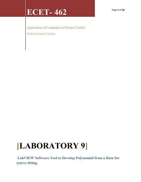
ECET- 462<br />
Page 1 of 10<br />
Application of Computers in Process Control<br />
Purdue University, Calumet<br />
[LABORATORY 9]<br />
<strong>LabVIEW</strong> <strong>Software</strong> <strong>Tool</strong> <strong>to</strong> <strong>Develop</strong> <strong>Polynomial</strong> <strong>from</strong> a <strong>Data</strong> <strong>Set</strong><br />
(curve fitting
Page 2 of 10<br />
<strong>LabVIEW</strong> <strong>Software</strong> <strong>Tool</strong> <strong>to</strong> <strong>Develop</strong> <strong>Polynomial</strong> <strong>from</strong> a <strong>Data</strong> <strong>Set</strong><br />
(curve fitting<br />
LAB 9<br />
Objective:<br />
To demonstrate the use of Lab View for <strong>Polynomial</strong> curve fitting.<br />
<strong>Software</strong> required: Lab View.<br />
Procedure:<br />
Step 1: Open Lab ViewCreate a new viSave it as Polyfit.<br />
Step 2: Go <strong>to</strong> Block diagram by pressing ‘Cntrl+E’. Go <strong>to</strong><br />
FunctionsMathematicsFitting General <strong>Polynomial</strong> fit.vi<br />
Place it on<strong>to</strong> block diagram.
Page 3 of 10<br />
Step 2: Create ‘Control’ <strong>from</strong> ‘X’, ‘Y’ and ‘<strong>Polynomial</strong> order’ terminals <strong>from</strong> the block. And<br />
also create an ‘Indica<strong>to</strong>r’ <strong>from</strong> the ‘Best <strong>Polynomial</strong> Fit’ terminal.<br />
Step 3: Go <strong>to</strong> Mathematics<strong>Polynomial</strong><strong>Polynomial</strong> Evaluation.vi<br />
Again go <strong>to</strong> Signal Processingsignal generationRamp pattern.vi<br />
Place these two blocks in the block diagram and connect as shown below. Create constants <strong>from</strong><br />
the start, end and samples terminals.
Page 4 of 10<br />
Step 4: Now take two blocks of bundle and a block of Build Array. Connect them as in the figure<br />
below.<br />
Programming Cluster, Class & Variant Bundle.<br />
Programming Array Build Array. Stretch the bundle <strong>to</strong> make two inputs.
Page 5 of 10<br />
Step 5: Place one ‘Reverse 1D Array’, one ‘CD construct Transfer function Model’ and one ‘CD<br />
draw Transfer function Equation’ <strong>from</strong> the destinations shown below and connect them as in<br />
figure. The ‘output’ of reverse 1D array should be connected <strong>to</strong> the ‘numera<strong>to</strong>r’ terminal of CD<br />
construct Transfer function Model. And the ‘Transfer Function Model’ terminal of CD construct<br />
Transfer function Model should be connected <strong>to</strong> the ‘Transfer Function Model’ terminal of the<br />
CD draw Transfer function Equation block.<br />
Step 6: Create an Indica<strong>to</strong>r <strong>from</strong> Equation terminal and a constant <strong>from</strong> Function Name Terminal<br />
of the CD draw Transfer function Equation block.
Page 6 of 10<br />
Step 7: Now go <strong>to</strong> the front Panel and rearrange the items as in figure. In order <strong>to</strong> increase the<br />
number of rows, stretch the block.<br />
Step 8: From the Controls pallete place a XY graph in the front panel.
Page 7 of 10<br />
Step 9: Go <strong>to</strong> block diagram panel. There find the XY graph and connect it <strong>to</strong> the build array.<br />
Right click on the graph and go <strong>to</strong> the destination indicated below.<br />
Step 9: Place the XY graph Cursor Position and create an Indiac<strong>to</strong>r
Page 8 of 10<br />
Step 10: Now right click on the xy graph and select properties. From the Graph Properties select<br />
the indicated properties.
Page 9 of 10<br />
Step 11: Now go <strong>to</strong> the Front panel and change the name of x and y axis <strong>from</strong> their default name<br />
of ‘Time’ and ‘Amplitude’ <strong>to</strong> some other name. Write down some values in the empty x and y<br />
column and run the program.<br />
Step 12: To do Extrapolation create a control <strong>to</strong> the ramp genera<strong>to</strong>rs End terminal (go <strong>to</strong> block<br />
diagram panel). Go <strong>to</strong> the front panel and change the value of end block and you will able <strong>to</strong> see<br />
the predictate values due <strong>to</strong> extrapolation.
Page 10 of 10<br />
Step 13: Move your cursor along the curve and you will get the values of x and y for the<br />
corresponding change in cursor position.<br />
Report:<br />
1. Why do we need a ramp genera<strong>to</strong>r in this program?<br />
2. Continue <strong>to</strong> increase polynomial order keeping other terms constant. What does happen?<br />
Why?<br />
3. State some applications of this program.