Risk 1 - Hans Buehler

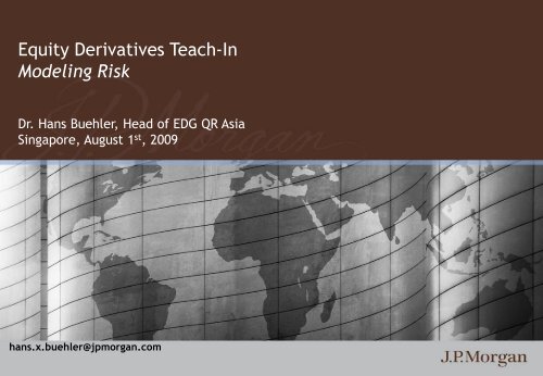
Equity Derivatives Teach-In 

Modeling Risk 

Dr. Hans Buehler, Head of EDG QR Asia 

Singapore, August 1 st , 2009 

hans.x.buehler@jpmorgan.com 

0

English_General 

[ P R E S E N T A T I O N T I T L E ] 

This presentation was prepared exclusively for the benefit and internal use of the J.P. Morgan client to whom it is directly addressed and delivered (including such 

client’s subsidiaries, the ―Company‖) in order to assist the Company in evaluating, on a preliminary basis, the feasibility of a possible transaction or transactions 

and does not carry any right of publication or disclosure, in whole or in part, to any other party. This presentation is for discussion purposes only and is 

incomplete without reference to, and should be viewed solely in conjunction with, the oral briefing provided by J.P. Morgan. Neither this presentation nor any of 

its contents may be disclosed or used for any other purpose without the prior written consent of J.P. Morgan. 

The information in this presentation is based upon any management forecasts supplied to us and reflects prevailing conditions and our views as of this date, all of 

which are accordingly subject to change. J.P. Morgan’s opinions and estimates constitute J.P. Morgan’s judgment and should be regarded as indicative, 

preliminary and for illustrative purposes only. In preparing this presentation, we have relied upon and assumed, without independent verification, the accuracy 

and completeness of all information available from public sources or which was provided to us by or on behalf of the Company or which was otherwise reviewed by 

us. In addition, our analyses are not and do not purport to be appraisals of the assets, stock, or business of the Company or any other entity. J.P. Morgan makes 

no representations as to the actual value which may be received in connection with a transaction nor the legal, tax or accounting effects of consummating a 

transaction. Unless expressly contemplated hereby, the information in this presentation does not take into account the effects of a possible transaction or 

transactions involving an actual or potential change of control, which may have significant valuation and other effects. 

Notwithstanding anything herein to the contrary, the Company and each of its employees, representatives or other agents may disclose to any and all persons, 

without limitation of any kind, the U.S. federal and state income tax treatment and the U.S. federal and state income tax structure of the transactions 

contemplated hereby and all materials of any kind (including opinions or other tax analyses) that are provided to the Company relating to such tax treatment and 

tax structure insofar as such treatment and/or structure relates to a U.S. federal or state income tax strategy provided to the Company by J.P. Morgan. 

J.P. Morgan’s policies prohibit employees from offering, directly or indirectly, a favorable research rating or specific price target, or offering to change a rating or 

price target, to a subject company as consideration or inducement for the receipt of business or for compensation. J.P. Morgan also prohibits its research analysts 

from being compensated for involvement in investment banking transactions except to the extent that such participation is intended to benefit investors. 

IRS Circular 230 Disclosure: JPMorgan Chase & Co. and its affiliates do not provide tax advice. Accordingly, any discussion of U.S. tax matters included 

herein (including any attachments) is not intended or written to be used, and cannot be used, in connection with the promotion, marketing or 

recommendation by anyone not affiliated with JPMorgan Chase & Co. of any of the matters addressed herein or for the purpose of avoiding U.S. tax-related 

penalties. 

J.P. Morgan is a marketing name for investment banking businesses of JPMorgan Chase & Co. and its subsidiaries worldwide. Securities, syndicated loan arranging, 

financial advisory and other investment banking activities are performed by a combination of J.P. Morgan Securities Inc., J.P. Morgan plc, J.P. Morgan Securities 

Ltd. and the appropriately licensed subsidiaries of JPMorgan Chase & Co. in Asia-Pacific, and lending, derivatives and other commercial banking activities are 

performed by JPMorgan Chase Bank, N.A. J.P. Morgan deal team members may be employees of any of the foregoing entities. 

This presentation does not constitute a commitment by any J.P. Morgan entity to underwrite, subscribe for or place any securities or to extend or arrange credit or 

to provide any other services. 

1

Contents 

• Introduction, Overview, Product Lifecycle 

• Products 

• Modeling Risk 

— Basics 

— Local Volatility 

— Stochastic Volatility 

— Crash Risk 

• Numerical Methods 

2

Contents 

Challenges in Equity Modelling 

• Deterministic 

— Implied Volatility 

— Interest rates 

— Dividend marks and handling 

(proportional vs. discrete) 

— FX Volatilities 

— Equity Correlation 

— Equity/FX Correlation 

— Repo, borrow, basis, etc 

• First Order 

— Local Volatility 

— CDS/Credit risk 

• Second Order 

— Stochastic Volatility / Jumps 

— Stochastic Dividends 

— Stochastic Interest rates 

— Equity/IR correlation 

• Third Order 

— Stochastic Correlation 

— Stochastic Credit Risk 

— Equity/Credit ―correlation‖ 

• Fourth Order 

— Transaction Costs, Liqudity 

— Forward curve models 

3


Basics 

4

Modeling Risk – Basics 

Setting 

• Given is a Stochastic Differential Equation 

Brownian 

Motion 

dS( 

t) 

S( 

t) 

= ( 

t) 

dt s ( t, 

S( 

t)) 

dW ( t) 

Drift 

Volatility 

Forward 

— In the risk-neutral world, the drift is implied by E[S(t)] = F(t) as 

dF( 

t) 

( t) 

dt = r( 

t) 

 

( t) 

F( 

t) 

— Black & Scholes [3]: s= s BS is a constant number. 

5


Black & Scholes 

1400 

S&P500 versus Geometric Brownian Motion 

1300 

1200 

1100 

1000 

900 

800 

One of these paths 

is the actual S&P 

500, the other two 

are simulated using 

Black & Scholes. 

28/06/2003 06/10/2003 14/01/2004 23/04/2004 01/08/2004 09/11/2004 17/02/2005 28/05/2005 05/09/2005 14/12/2005 

6



• For this particular choice, the SDE has the analytical solution 

S 

BS 

1 2 

( t) 

= F( 

t)exp 

s 

BSW 

( t) 

s 

BS 

t 

2 

which allows computing vanilla option prices and, indeed, many more 

option prices analytically. 

The famous Black&Scholes formula for the value of an European call is: 

FV( T,Stoday) 

: = 

DF( T) 

= DF( T) 

E 

 

 

 

S 

BS 

( T) 

K 

F(T)N ( d 

 

 

 

 

) KN( 

d 

 

) 

d 

 

= 

ln( F( 

T) / K) 

 

s 

BS 

T 

1 

2 

s 2 

BS 

T 

7



• The value of each payoff under Black&Scholes is a function of the current 

spot level S today and time-to-maturity T: 

FV( T,Stoday) : = DF( T) 

E F( 

S ( T) 

 

t, S) : = FV( t, 

S) 

S 

— The seminal paper of Black&Scholes has shown that if the market is 

behaving like the model predicted, then perfect replication is possible: 

 

BS 

 

Payoff at 

maturity T 

 

S( 

T) 

K = FV(0, S ) 

Fair Value of 

the option 

today (time 0) 

T 

today 

( t, 

S( 

t)) 

dS( 

t) 

0 

Delta-Hedging 

(*) This simplified 

formula holds if 

•Interest rates are zero 

•The stock pays mo 

dividends 

•The stock earns/pays 

no borrow 

8



• What does this formula mean? 

S( 

T) 

K = FV(0, S ) ( t, 

S( 

t)) 

dS( 

t) 

— It tells us how to execute the hedge: 

FV( 

t 

 

today 

1 

dt, 

S( 

t1)) 

= FV(0, Stoday) 

(0, 

Stoday) 

S( 

t1) 

T 

0 

 

S 

today 

 

Buy units of 

shares today 

and sell them 

tomorrow. 

Tomorrow’s 

option value 

— For two days: 

Today’s option 

value 

9



• What does this formula mean? 

— For two days: 

FV( t 

2 

= FV( t 

, S( 

t 

1 

, S( 

t 

= FV(0, S 

 

S( 

T) 

K = FV(0, S ) ( t, 

S( 

t)) 

dS( 

t) 

2 

)) 

1 

today 

)) ( 

t 

1 

, S( 

t 

) (0, 

S 

1 

)) 

today 

) 

 

S( 

t 

2 

today 

) S( 

t 

) 

T 

0 

 

S 

( t ) S ( 

t , S( 

t )) S 

( t ) S( 

t ) 

1 

1 

today 

1 

1 

2 

1 

10



• The formula is understood as 

Change of 

option value 

Change of 

Delta position 

value 

FV( t 

dt, 

S( 

t 

dt)) 

FV( t, 

S( 

t)) 

dFV( 

t) 

= 

= 

( 

t, 

S( 

t)) 

 

S( 

t 

( 

t) 

dS( 

t) 

dt) 

S( 

t) 

 

• Practitioners often look at ―cash delta‖ rather than delta. 

It reflects the cash value of the delta position: 

— This gives 

 

$ 

( t) : = 

dFV( 

t, 

S( 

t)) 

= 

( 

t) 

S( 

t) 

 

$ 

dS( 

t) 

( t) 

S( 

t) 

Return on the 

stock 

investment 

11

Fair Value 

-200% 

-180% 

-160% 

-140% 

-120% 

-100% 

-80% 

-60% 

-40% 

-20% 

0% 

20% 

40% 

60% 

80% 

100% 

120% 

140% 

160% 

180% 

200% 


4 

Hedging a European Call 

(3d to maturity, 45% Volatility) 

Price T 

3 

Price(S0) + Delta T 

Price T+1 

2 

1 

Break-Even 

Point at 

-100% 

Break-Even 

Point at 

+100% 

0 

Stock price move in standard deviations 

(relative to one-day volatility) 

12

Daily Return / Initial Fair Value 


40% 

Naked European Call (matures 99% OTM) 

30% 

20% 

10% 

0% 

-10% 

-20% 

Using actual 

-30% 

HSI market 

04-Jul-08 04-Sep-08 04-Nov-08 04-Jan-09 04-Mar-09 data 04-May-09 

13



40% 

Delta-Hedging an European Call 

30% 

20% 

Unhedged 

Hedged 

10% 

0% 

-10% 

-20% 

-30% 

04-Jul-08 04-Sep-08 04-Nov-08 04-Jan-09 04-Mar-09 04-May-09 

14



40% 

Delta-Hedging an European Call 

500% 

30% 

20% 

LogSqRet 

Unhedged 

450% 

400% 

350% 

10% 

Hedged 

300% 

250% 

0% 

200% 

-10% 

-20% 

High daily 

volatility leads 

to deterioration 

of hedging 

performance. 

150% 

100% 

50% 

-30% 

04-Jul-08 04-Sep-08 04-Nov-08 04-Jan-09 04-Mar-09 04-May-09 

0% 

15

Probability 


70% 

Effect of Delta Hedging on the Return Distribution for ATM Calls 

60% 

50% 

40% 

30% 

Unhedged 2w 

Unhedged 1m 

Unhedged 2m 

Hedged 2w 

Hedged 1m 

Hedged 2m 

20% 

10% 

Marked 

reduction 

in tail risk 

Marked 

reduction 

in tail risk 

0% 

-50% -43% -37% -30% -23% -17% -10% -3% 3% 10% 17% 23% 30% 37% 43% 50% 

__ 

Period Feb 06 – April 07 

16



• What about the error if we only hedge daily (not instantaneous) ? 

— Black&Scholes PDE: 

dFV( 

t) 

 

$ 

( t) 

dS( 

t) 

S( 

t) 

= 

1 

2 

 

$ 

2 

dS( 

t) 

 

 

S( 

t) 

 

dt 

“Cash Gamma” 

$ := S 2 

Theta 

• Key message 

— Theta ―compensates‖ for Gamma (theta is negative – the option value 

decays in time) 

— The hedge works perfectly if Theta and the Gamma term cancel. 

17


Black & Scholes – Break Even Vol 

• In a Black&Scholes world, the hedge works perfectly, 

• Hence, Theta must cancel if the asset squared return is just as anticipated 

by the Black&Scholes model – this means: 

dFV( 

t) 

 

( t) 

dS( 

t) 

S( 

t) 

• Define the ―Break Even Volatility‖ 

$ 

s 

2 

break even 

= 

= 

1 

 

2 

1 

 

2 

$ 

$ 

2 

dS( 

t) 

 

 

S( 

t) 

 

 

s s 

2 

realized 

 

2 

dt 

: = 

$ 

dt 

2 

BS 

dt 

18


Black & Scholes – Break Even Vol 

• Break Even Vol 

— Note that for practical computation, needs to be computed carefully; 

the so-called ―optionality theta‖ is the raw theta 

 

optionalit y 

= 

simpleshift 

{dividends 

funding 

client cashflows} 

• In other words, 

s 

2 

break even 

 

optionalit y 

: = 

$ 

2 

dt 

19


Black & Scholes – Summary Break Even Vol 

• The most basic equation of Modeling Risk 

dFV( 

t) 

 

$ 

( t) 

dS( 

t) 

S( 

t) 

= 

1 

2 

 

$ 

 

s 

2 

realized 

s 

2 

model 

dt 

— Holds for all one-factor stock price models (*) 

dS( 

t) 

S( 

t) 

= ( 

t) 

dt s ( t, 

S( 

t)) 

dW ( t) 

— A similar formula will be shown for stochastic volatility 

We say ―we pay Theta‖ for the Gamma of the option. 

__ 

(*) assuming no daily recalibration. 

20


Local Volatility 

21

Modeling Risk – Local Volatility 

Black & Scholes – Implied Volatility 

• Recall the Black&Scholes formula for a European call: 

FV( T,Stoday) 

: = 

DF( T) 

= DF( T) 

E 

 

 

 

S 

BS 

( T) 

K 

F(T)N ( d 

 

 

 

 

) KN( 

d 

 

) 

d 

 

= 

ln( F( 

T) / K) 

 

s 

BS 

T 

1 

2 

s 2 

BS 

T 

22

Implied Vol 

8346 

9737 

11128 

12519 

13910 

15301 

16692 

18083 

19474 



• Using the BS volatility s BS as a free parameter, we can invert the BS 

formula to back out the so-called ―BS implied volatility‖ surface of the 

Market 

market. 

70% 

60% 

50% 

40% 

30% 

1Y 

2Y 

3Y 

3M 

Strike 

Example: HSI Mar 25, 2009 @ 13,910 

23



s Τ 

Κ 

= s 

ATM 

Τ 

Κ 

2 

K 1 

K 

skew* ln 

convexity *ln 

 

F( 

T) 

2 

F( 

T) 

 

approximately 

s ( T,105%) 

s ( T,95%) 

skew = 

10% 

for 95/105 strikes relative to forward (what we used before). 

Formula does not hold for far OTM strikes. 

24


Recall: Pricing with Skew 

0.7 

Skew Impact on ATM Digital Puts (95-105 skew @ -5%) 

0.6 

0.5 

0.4 

0.3 

0.2 

0.1 

0 

Digital 

Put Spread 0.01% 



Put Spread 1% 

1w 1m 3m 6m 1y 

25

Implied Vol 

8346 

9737 

11128 

12519 

13910 

15301 

16692 

18083 

19474 



• Observed market option prices are not consistent with the BS assumption of 

a single constant volatility, and not even with the assumption of a timedependent 

volatility. 

Market 

70% 

60% 

50% 

40% 

30% 

1Y 

2Y 

3Y 

3M 

Strike 

Any pricing algorithm needs to “re-price” the observed option prices 

(otherwise we would have internal arbitrage). 

26


Dupire’s Local Volatility 

• Classic Solution: Dupire’s Local Volatility [2] 

the second most used model in equity derivatives 

— Idea: find s as a function of spot and time such that 

dS 

S 

LV 

LV 

( t) 

( t) 

= ( 

t) 

dt s 

LV 

( t, 

S 

LV 

( t)) 

dW ( t) 

reprices all market prices, ie 

 

 

! 

 

S ( t) 

K MarketCallPrice( t, 

K) 

DF( t) 

E 

LV 

= 

27



• Key points 

— Dupire’s local volatility is unique within the class of diffusions 

— In this class it is well-defined and given as 

where 

s ( t, 

S): 

= ~ 

LV 

s 

~ s 

LV 

 

t, 

k 

 

2 

: = 

LV 

2k 

~ 

C( 

t, 

k) 

t 

2 

~ 

C( 

t, 

k) 

2 

k 

2 

 

t, 

 

S 

F( 

t) 

 

 

 

Normalized 

Call Prices 

~ 

C ( t, 

k) 

: = 

MarketCallPrice t,kF( 

t) 

DF( t) 

F( 

t) 

 

 

28



Implied Volatility SPX Dec 9 2005 

Local Volatility SPX 

80 

80 

70 

70 

60 

60 

50 

50 

40 

40 

30 

20 

10 

0 

09-Dec-18 

09-Jun-16 

09-Dec-13 

09-Jun-11 

09-Dec-08 

30 

20 

10 

0 

09-Jun-18 

09-Dec-15 

09-Jun-13 

09-Dec-10 

09-Jun-08 

09-Jun-06 

09-Dec-05 

Strike/Spot 

Strike/Spot 

29

Implied Volatility 

Implied Volatility 


Dupire’s Local Volatility – time dependency 

Implied Vol 

flattens out in the 

future inside the 

Local Vol Model 

Local Vol Calibration .STOXX50E 10/10/2005 

Local Vol Calibration .STOXX50E 10/10/2005 shifted forward by 2 years 

50.0 

50.0 

45.0 

45.0 

40.0 

40.0 

35.0 

35.0 

30.0 

30.0 

25.0 

20.0 

15.0 

10.0 

5.0 

0.0 

70% 80% 90% 100% 110% 120% 130% 

Strike/Spot 

1m 

4m 

1y 

25.0 

20.0 

15.0 

10.0 

5.0 

0.0 

70% 

80% 

90% 

100% 

Strike/Spot 

110% 

120% 

130% 

1m 

3m 

6m 

1y 

30



• Plus 

— Allows to consistently price all combinations of European options. 

— One-factor model fast to simulate 

— Break Even Vol formula applies 

• Cons 

— Dynamical behaviour is not consistent 

— Implied Vol needs to be sensible 

Widely used reference model for equity derivatives. 

31

Thank you very much for your attention. 

hans.x.buehler@jpmorgan.com 

32

Numerical Methods 

References 

— [1] Gatheral: The Volatility Surface, Wiley, 2006 

— [2] Dupire: Pricing with a Smile, Risk, 7 (1), pp. 18-20, 1996 

— [3] Black, Scholes: The Pricing of Options and Corporate Liabilities, Journal of Political 

Economy, 81, pp. 637-59, 1973 

— [4] Carr, Madan: Option Valuation Using the Fast Fourier Transform, Journal of Computational 

Finance, 2, 1998 

— [5] Ren, Madan, Qian: Calibrating and pricing with embedded local volatility models, Risk, 

September 2007 

— [6] Buehler, Volatility Markets, VDM Verlag, 2008 

— [7] Merton: Option Pricing When Underlying Stock Returns are Discontinuous. Journal of 

Financial Economics 3 (1976) pp. 125-144, 1976 

— [8] Cont, Tankov: ―Financial modeling with Jump Processes‖, Chapman & Hall / CRC Press, 

2003 

— [9] Buehler, Volatility and Dividends, Working paper, 2008, http://www.math.tuberlin.de/~buehler/ 

— [10] Glasserman, ―Monte Carlo Methods in Financial Engineering‖, Springer 2004 

— [11] Andersen, Piterbarg: Moment Explosions in Stochastic Volatility Models WP~2004, 

http://ssrn.com/abstract=559481 

— [12] Bermudez, Buehler, Ferraris, Jordinson, Lamnouar, Overhaus: ―Equity Hybrid 

Derivatives‖, Wiley, 2006 

33

Risk 1 - Hans Buehler

Create successful ePaper yourself

Delete template?

Save as template?