Unfiltered FQPSK: Another Interpretation and Further Enhancements

Unfiltered FQPSK: Another
Interpretation and Further
Enhancements
Part 1: Transmitter implementation and optimum reception
By Marvin K. Simon and Tsun-Yee Yan
Jet Propulsion Laboratory
Anew interpretation of unfiltered Feher-
Patented Quadrature Phase-Shift-Keying
(FQPSK) is presented, readily identifying
a means for spectral enhancement of the transmitted
waveform as well as an improved method
of reception. The key to these successes is the
replacement of the half-symbol by half-symbol
mapping, originally used to describe FQPSK by
a symbol-by-symbol mapping operation combined
with memory. The advantages of such an
interpretation are two-fold. In particular, the
original FQPSK scheme can be modified so that
the potential of a waveform slope discontinuity
at the boundary between half symbols is avoided
without sacrificing the “constant” envelope
property of the transmitted waveform. Also, a
memory receiver can be employed to improve
error probability performance relative to previously
proposed symbol-by-symbol detection
methods. The analysis presented in this paper
does not include other versions of FQPSK, such
as FQPSK-B, which is currently being considered
for military applications.
This is part one of a two-part article. Part two
will be published in the March 2000 issue of
Applied Microwave & Wireless magazine.
Introduction
In its generic form, Feher-Patented
Quadrature Phase-Shift-Keying (FQPSK), as
patented [1] and reported in the recent literature
[2-3], is conceptually the same as the crosscorrelated
phase-shift-keying (XPSK) modulation
technique introduced in 1983 by Kato and
Feher [4]. 1 This technique was in turn a modification
of the previously introduced (by Feher et
al [6]) interference and jitter free QPSK (IJF-
QPSK), with the express purpose of reducing
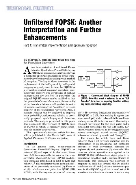
▲ Figure 1. Conceptual block diagram of FQPSK
(XPSK). Note that what is referred to as an “IJF
Encoder” is in fact a mapping function without
any error-correcting capability.
the 3 dB envelope fluctuation characteristic of
IJF-QPSK to 0 dB, thus making it appear constant
envelope 2 , which is beneficial in nonlinear
radio systems. (It is further noted that using a
constant waveshape for the even pulse and a
sinusoidal waveshape for the odd pulse, IJF-
QPSK becomes identical to the staggered quadrature
overlapped raised cosine (SQORC)
scheme introduced by Austin and Chang [7]).
The means by which Kato and Feher
achieved their 3 dB envelope reduction was the
introduction of an intentional but controlled
amount of cross correlation between the
inphase (I) and quadrature (Q) channels. This
cross correlation operation was applied to the
IJF-QPSK (SQORC) baseband signal prior to its
modulation onto the I and Q carriers (Figure 1).
Specifically, this operation was described by
mapping in each half symbol the 16 possible
combinations of I and Q channel waveforms present
in the SQORC signal into a new 3 set of 16
waveform combinations, chosen in such a way
76 · APPLIED MICROWAVE & WIRELESS

that the cross correlator output is time continuous and
has unit (normalized) envelope 4 at all I and Q uniform
sampling instants.
Because the cross correlation mapping is based on a
half symbol characterization of the SQORC signal, there
is no guarantee that the slope of the cross correlator output
waveform is continuous at the half symbol transition
points. In fact, we will show that for a random data
input sequence, such a discontinuity in slope occurs one
quarter of the time.
It is well known that the rate at which the side lobes
of a modulation’s power spectral density (PSD) roll off
with frequency is related to the smoothness of the
underlying waveforms that generate it. That is, the
more derivatives of a waveform that are continuous, the
faster its Fourier transform decays with frequency.
Thus, since the first derivative of the FQPSK waveform
is discontinuous (at half symbol transition instants) on
the average one quarter of the time, one can anticipate
that an improvement in PSD rolloff could be achieved if
the FQPSK cross correlation mapping could be modified
so the first derivative is always continuous.
Restructuring the cross correlation mapping into a
symbol-by-symbol representation will place the slope
discontinuity referred to above in evidence and will be
particularly helpful in suggesting a means to eliminate
it. This representation also has the advantage that it can
be described directly in terms of the data transitions on
the I and Q channels. Thus, the combination of IJF
encoder and cross correlator can be replaced simply by a
single modified cross correlator. The replacement of the
conventional FQPSK cross correlator by this modified
cross correlator, which eliminates the slope discontinuity,
leads to what we shall refer to as enhanced FQPSK.
We will show that not only does enhanced FQPSK have
a better PSD (in the sense of reduced out-of-band energy)
than conventional FQPSK, but from a modulation
symmetry standpoint, it is a more logical choice.
A further and more important advantage of the reformulation
as a symbol-by-symbol mapping is the ability
to design a receiver of FQPSK or enhanced FQPSK that
specifically exploits the correlation introduced into the
modulation scheme to significantly improve power efficiency
or equivalently, error probability performance.
Such a receiver, which takes a form analogous to those
used for trellis-coded modulations, will be shown to yield
significant performance improvement over receivers
that employ symbol-by-symbol detection, thus ignoring
the inherent memory of the modulation.
Review of IJF-QPSK and SQORC
The IJF-QPSK scheme (alternately called FQPSK-1)
is based on defining waveforms s o (t) and s e (t), which are
respectively odd and even functions of time over the
symbol interval –T s /2 ≤ t ≤ T s /2, and then using these
and their negatives –s o (t), –s e (t) as a 4-ary signal set for
▲ Figure 2a. Inphase IJF encoder output.
▲ Figure 2b. Quadrature phase IJF encoder output.
transmission in accordance with the values of successive
pairs of data symbols in each of the I and Q arms.
Specifically, if d In denotes the I channel data symbols in
the interval, (n–½)T s ≤ t ≤ (n+½)T s , then the transmitted
waveform x I (t) in this same interval would be determined
as follows:
x I (t)=s e (t–nT s )= ∆ s 0 (t–nT s ) if d I,n–1 =1, d I,n =1
x I (t)=–s e (t–nT s )= ∆ s 1 (t–nT s ) if d I,n–1 =–1, d I,n =–1
x I (t)=s o (t–nT s )= ∆ s 2 (t–nT s ) if d I,n–1 =–1, d I,n =1
x I (t)=–s o (t–nT s ) = ∆ s 3 (t–nT s ) if d I,n–1 =1, d I,n =–1
The Q channel waveform x Q (t) would be generated by
the same mapping as in (1) using instead the Q channel
data symbols {d Qn } and then delaying the resulting
waveform by one half a symbol. If the odd and even
waveforms s o (t) and s e (t) are defined by
se() t = 1, −Ts / 2≤ t ≤Ts
/ 2
πt
so( t) = sin , −Ts
/ 2≤ t ≤Ts
/ 2
T
s
(1)
(2)
78 · APPLIED MICROWAVE & WIRELESS

then typical waveforms for the I and Q IJF encoder outputs
are illustrated in Figure 2.
An identical modulation to x I (t) (and likewise for
x Q (t)) generated from the combination of (1) and (2) can
be obtained directly from the binary data sequence {d In }
itself, without the need for defining a 4-ary mapping
based on the transition properties of the sequence. In
particular, if we define the two-symbol wide raised
cosine pulse shape
pt ( ) = sin
then the I modulation
x () t = ∑ d p( t−
nT)
I
will be identical to that generated by the above IJF
scheme. Similarly,
⎛ ⎞
x () t = d p( t n T)
Q ∑ − +
Qn
s
n=−∞
⎝ 2⎠
∞ 1
(a)
(c)
∞
n=−∞
( )
⎛ π t+
T /
⎜
⎝ 2T
2 s 2
In
s
⎞
⎟, −Ts
/ 2≤ t ≤3Ts
/ 2
⎠
s
(b)
(d)
(3)
(4)
(5)
would also be identical to that generated by the above
IJF scheme. A quadrature modulation scheme formed
from x I (t) of (4) and x Q (t) of (5) is precisely what Austin
and Chang [7] referred to as SQORC modulation, namely,
independent I and Q modulations with overlapping
raised cosine pulses on each channel. The resulting carrier
modulated waveform is described by
xt () = x1()cos t ωct+
xQ()sin
t ωct
Symbol-by-symbol cross correlator mapping for FQPSK
Before revealing the modification of FQPSK, which
results in a transmitted signal having a continuous first
derivative, we first recast the original characterization
of FQPSK in terms of a cross correlation operation performed
on the pair of IJF encoder outputs every half
symbol interval into a mapping performed directly on
the input I and Q data sequences every full symbol interval.
To do this, we define sixteen waveforms
s i (t);i=0,1,2,...,15 over the interval –T s /2 ≤ t ≤ Τ s /2,
which collectively form a transmitted signaling set for
the I and Q channels. The particular I and Q waveforms
chosen for any particular T s -sec signaling interval on
each channel depends on the most recent data transition
on that channel as well as the two most recent successive
transitions on the other channel (Figure 3).
s () t = A, −T /
s
2≤ t ≤ T /
s
2, s () t = −s () t
0 8 0
⎧A, −T / 2≤ s
t ≤0
⎪
s()
1
t = ⎨
2 πt
,
⎪
1−( 1−
A) cos , 0≤ t ≤T
/ 2
s
⎩
Ts
s ()
9
t =−s()
1
t
⎧
2 π t
⎪1−( 1−
A)cos
, −Ts
/ 2≤ t ≤0
s () t =
T
2 ⎨
s
,
⎪
⎩A. 0≤
t ≤Ts
/ 2
s10() t =−s2()
t
2 πt
s ( t) = −( − A)cos , −Ts
/ ≤ t ≤Ts
/
3
1 1 2 2 ,
Ts
s () t =−s () t
11
3
(6)
(7a)
(e)
(g)
(f)
(h)
▲ Figure 3. FQPSK full-symbol waveforms: (a) s 0 (t) = –s 8 (t)
vs. t; (b) s 1 (t) = –s 9 (t) vs t; (c) s 2 (t) = –s 10 (t) vs. t; (d) s 3 (t)
= –s 11 (t) vs. t; (e) s 4 (t) = –s 12 (t) vs. t; (f) s 5 (t) = –s 13 (t)
vs. t; (g) s 6 (t) = –s 14 (t); and (h) s 7 (t) = –s 15 (t) vs. t.
πt
s4( t) = Asin , −Ts
/ 2≤ t ≤Ts
/ 2
T
s
12
s
() t =−s () t
⎧ πt
Asin , −Ts
/ 2≤ t ≤0
⎪ Ts
s5()
t = ⎨
⎪ πt
sin , 0≤
t ≤Ts
/ 2
⎩⎪
Ts
s () t =−s () t
13
⎧ πt
sin , − Ts
/ 2 ≤ t ≤0
⎪ Ts
s6()
t = ⎨
⎪ πt
Asin , 0 ≤ t ≤Ts
/ 2
⎩⎪
Ts
s () t =−s () t
πt
s7
( t) = sin , −Ts
/ 2≤ t ≤Ts
/ 2
T
s
14
15
s
5
6
4
() t =−s () t
7
,
,
,
,
(7b)
80 · APPLIED MICROWAVE & WIRELESS

Note that for any value of A other
then unity, s 6 (t) and s 7 (t) as well as
their negatives s 13 (t) and s 14 (t), will
have a discontinuous slope at their
midpoints (i.e., at t=0), whereas the
remaining twelve waveforms all
have a continuous slope throughout
their defining interval. Also, all 16
waveforms have zero slope at their
endpoints, and thus concatenation
of any pair of these will not result in
a slope discontinuity.
Next, we define the mapping
function for the baseband I-channel
transmitted waveform y 1 (t)=s I (t) in
the nth signaling interval (n–½)T s ≤
t ≤ (n+½)T s , in terms of the transition
properties of the I and Q data
symbol sequences {d In } and {d Qn },
respectively.
8a
I. If d I,n–1 =1, d I,n =1 (no transition
on the I sequence, both data bits
positive), then
A. y I (t)=s 0 (t–nT s ) if d Q,n–2 , d Q,n–1 ,
results in no transition and d Q,n–1 ,
d Q,n results in no transition.
B. y I (t)=s 1 (t–nT s ) if d Q,n–2 , d Q,n–1
results in no transition and d Q,n–1 ,
d Q,n results in a transition (positive
or negative).
C. y I (t)=s 2 (t–nT s ) if d Q,n–2 , d Q,n–1
results in a transition (positive or
negative) and d Q,n–1 , d Q,n results in
no transition.
D. y I (t)=s 3 (t–nT s ) if d Q,n–2 , d Q,n–1
results in a transition (positive or
negative) and d Q,n–1 , d Q,n results in a
transition (positive or negative).
8b
II. If d I,n–1 =–1, d I,n =1 (a positive
going transition on the I sequence),
then
A. y I (t)=s 4 (t–nT s ) if d Q,n–2 , d Q,n–1
results in no transition and d Q,n–1 ,
d Q,n results in no transition.
B. y I (t)=s 5 (t–nT s ) if d Q,n–2 , d Q,n–1
results in no transition and d Q,n–1 ,
d Q,n results in a transition (positive
or negative).
C . y I (t)=s 6 (t–nT s ) if d Q,n–2 , d Q,n–1
results in a transition (positive or
negative) and d Q,n–1 , d Q,n results in
no transition.
D. y I (t)=s 7 (t–nT s ) if d Q,n–2 , d Q,n–1
results in a transition (positive or
negative) and d Q,n–1 , d Q,n results in a
transition (positive or negative).
8c
III. If d I,n–1 =–1, d I,n =–1(no transition
on the I sequence, both data bits
negative), then
A. y I (t)=s 8 (t–nT s ) if d Q,n–2 , d Q,n–1
results in no transition and d Q,n–1 ,
d Q,n results in no transition.
B. y I (t)=s 9 (t–nT s ) if d Q,n–2 , d Q,n–1
results in no transition and d Q,n–1 ,
d Q,n results in a transition (positive
or negative).
C. y I (t)=s 10 (t–nT s ) if d Q,n–2 , d Q,n–1
results in a transition (positive or
negative) and d Q,n–1 , d Q,n results in
no transition.
D. y I (t)=s 11 (t–nT s ) if d Q,n–2 ,
82 · APPLIED MICROWAVE & WIRELESS

d Q,n–1 results in a transition (positive
or negative) and d Q,n–1 , d Q,n
results in a transition (positive or
negative).
8d
IV. If d I,n–1 =1, d I,n =–1 (a negative
going transition on the I sequence),
then
A. y I (t)=s 12 (t–nT s ) if d Q,n–2 , d Q,n–1
results in no transition and d Q,n–1 ,
d Q,n results in no transition.
B. y I (t)=s 13 (t–nT s ) if d Q,n–2 , d Q,n–1
results in no transition and d Q,n–1 ,
d Q,n results in a transition (positive
or negative).
C. y I (t)=s 14 (t–nT s ) if d Q,n–2 , d Q,n–1
results in a transition (positive or
negative) and d Q,n–1 , d Q,n results in
no transition.
D. y I (t)=s 15 (t–nT s ) if d Q,n–2 , d Q,n–1
results in a transition (positive or
negative) and d Q,n–1 , d Q,n results in a
transition (positive or negative).
Making use of the signal properties
in (7a) and (7b), the mapping
conditions in (8a-8d) for the I channel
baseband output can be summarized
in a concise form (Table 1). A
similar construction for the baseband
Q-channel transmitted waveform
y Q (t) = s Q (t–T s /2) in the nth
signaling interval nT s ≤ t ≤ (n+1)T s
in terms of the transition properties
of the I and Q data symbol
sequences {d in } and {d Qn }, respectively,
can be obtained analogous to
(8a-d). The results are summarized
in Table 2. Note that the subscript i
of the transmitted signal s i (t–nT s ) or
s i (t–(n+½)T s ) as appropriate is the
binary coded decimal (BCD) equivalent
of the three transitions.
Applying the mappings in Tables
1 and 2 to the I and Q data
sequences of Figure 2 produces the
identical I and Q baseband transmitted
signals to those that would be
produced by passing the I and QIJF
encoder outputs of this figure
through the cross-correlator (half
symbol mapping) of the FQPSK
(XPSK) scheme as described in [4]
(Figure 4). Thus, we conclude that
for arbitrary I and Q input sequences,
FQPSK can alternately be generated
by the symbol-by-symbol mappings
of Tables 1 and 2 as applied to
these sequences.
A new and improved FQPSK
As discussed above, the symbolby-symbol
mapping representation
of FQPSK identifies the fact that
four out of the sixteen possible
transmitted waveforms, namely
s 5 (t), s 6 (t), s 13 (t) and s 14 (t) have a
slope discontinuity at their midpoint.
Thus, for random I and Q data
symbol sequences, on the average
the transmitted FQPSK waveform
will likewise have a slope discontinuity
at one quarter of the uniform
sampling time instants. To prevent
this from occurring, we now redefine
FEBRUARY 2000 · 83

▲ Figure 4a. Inphase FQPSK (XPSK) output.
▲ Figure 4b. Quadrature phase FQPSK (XPSK) output.
these four transmitted signals in a manner analogous to
s 1 (t), s 2 (t), s 9 (t) and s 10 (t), namely,
⎧ πt
2 πt
sin + ( 1− A)sin , −Ts
/ 2≤ t ≤0
⎪ Ts
Ts
s5()
t = ⎨
⎪ πt
sin , 0 ≤ t ≤Ts
/ 2
⎩⎪
Ts
s () t =−s () t
s
6
13
⎧ πt
sin , −Ts
/ 2≤ t ≤0
⎪ Ts
() t ⎨
⎪ πt
2 πt
sin −( 1 − A)sin , 0 ≤ t ≤Ts
/ 2
⎩⎪
Ts
Ts
s 14 () t =−s () t
6
5
Note that the signals s 5 (t), s 6 (t), s 13 (t) and s 14 (t) as
defined in (9) do not have a slope discontinuity at their
midpoint nor, for that matter, anywhere else in the
defining interval. Also, the zero slope at their endpoints
d In – d I,n–1 d Q,n–1 – d Q,n–2 d Qn – d Q,n–1 s I (t)
2 2 2
0 0 0 d In s 0 (t–nT s )
0 0 1 d In s 1 (t–nT s )
0 1 0 d In s 2 (t–nT s )
0 1 1 d In s 3 (t–nT s )
1 0 0 d In s 4 (t–nT s )
1 0 1 d In s 5 (t–nT s )
1 1 0 d In s 6 (t–nT s )
1 1 1 d In s 7 (t–nT s )
▲ Table 1. Mapping for inphase (I)-channel baseband signal
y I (t) in in the interval (n–½)T s ≤ t ≤ (n+½)T s .
,
,
(9)
has been preserved. Thus, using (9) in place of the corresponding
signals of (7b) will result in a modified
FQPSK signal that has no slope discontinuity anywhere
in time regardless of the value of A. Figure 5 illustrates
a comparison of the signal s 6 (t) of (9) with that of (7b)
for a value of A=1√2. Figure 6 illustrates the power spectral
density of conventional FQPSK and its enhancement
obtained by using the waveforms of (9) as replacements
for those in (7b). The significant improvement in
spectral rolloff rate is clear from a comparison of the
two.
As it currently stands, the signal set chosen for
enhanced FQPSK has a symmetry property for s 0 (t),
s 1 (t), s 2 (t) and s 3 (t) that is not present for s 4 (t), s 5 (t), s 6 (t)
and s 7 (t). In particular, s 1 (t) and s 2 (t) are each composed
of one half of s 0 (t) and one half of s 3 (t), i.e., the portion
of s 1 (t) from t = –T s /2 to t = 0 is the same as that of s 0 (t),
whereas the portion of s 1 (t) from t = 0 to t = T s /2 is the
same as that of s 3 (t), and vice versa for s 2 (t). To achieve
the same symmetry property for s 4 (t) – s 7 (t), one would
have to reassign s 4 (t) as
d Qn – d Q,n–1 d I,n – d I,n–1 d I,n+1 – d I,n s I (t)
2 2 2
0 0 0 d Qn s 0 (t–nT s )
0 0 1 d Qn s 1 (t–nT s )
0 1 0 d Qn s 2 (t–nT s )
0 1 1 d Qn s 3 (t–nT s )
1 0 0 d Qn s 4 (t–nT s )
1 0 1 d Qn s 5 (t–nT s )
1 1 0 d Qn s 6 (t–nT s )
1 1 1 d Qn s 7 (t–nT s )
▲ Table 2. Mapping for quadrature (Q)-channel baseband
signal y Q (t) in the interval nT s ≤ t ≤ (n+1)T s .
84 · APPLIED MICROWAVE & WIRELESS

▲ Figure 5. Original and new FQPSK shapes.
▲ Figure 6. Power spectra of conventional and enhanced FQPSK: (a)
without SSPA; and (b) with SSPA.
s
4
⎧ πt
2 πt
sin + ( 1− A)sin , −Ts
/ 2≤ t ≤0
⎪ Ts
Ts
() t = ⎨
,
⎪ πt
2 πt
sin −( 1− A)sin , 0 ≤ t ≤Ts
/ 2
⎩⎪
Ts
Ts
() t =−s () t
s 12
4
(10)
This minor change, which produces a complete symmetry
in the waveform set, has an advantage from the
standpoint of hardware implementation and produces a
negligible change in spectral properties of the transmitted
waveform. Nevertheless, for the remainder of the
discussion, we shall ignore this minor change and
assume the version of enhanced FQPSK first introduced
in this section.
Interpretation of FQPSK as a trellis-coded modulation
The I and Q mappings given in Tables 1 and 2 are
alternately described in terms of the (0,1) representation
of the I and Q data symbols and their transitions.
Specifically, define
D In = ∆ (1–d In )/2, D Qn = ∆ (1−d Qn )/2 (11)
which both range on the set (0,1). Then, defining the
BCD representation of the indices i and j by
with
3
i= I3
× 2 + I2
× 2 + I1
× 2 + I0
× 2
3
2
1
j= Q × 2 + Q × 2 + Q × 2 + Q × 2
3
I = DQn ⊕ D Q D D
0 Q n− , =
I n
⊕
, 1 0 , + 1 In
I = DQn , −
⊕ DQn , −
, Q = DIn⊕ DIn
, −
= I
I =
2
D ⊕
In
D ,
I n 1
Q =
2
D ⊕
Qn
D =
, −
Q,
n−1 I0
I = D , Q = D
1 1 2 1 1 2
3 In 3
2
2
Qn
1
(12)
(13)
we have y I (t)=s i (t–nT s ) and y Q (t)=s j (t–(n+½)T s ). That
is, in each symbol interval ((n–½)T s ≤ t ≤ (n+½)T s for
y I (t) and nT s ≤ t ≤ (n+1)T s for y Q (t)), the I and Q channel
baseband signals are each chosen from a set of 16
1
0
0
0
▲ Figure 7. Alternate implementation of FQPSK baseband signals.
▲ Figure 8. 16-state trellis diagram for FQPSK.
86 · APPLIED MICROWAVE & WIRELESS

signals, s i (t), i=0,1,...,15, in
accordance with the 4-bit
BCD representations of
their indices defined by (12)
together with (13). A graphical
illustration of the implementation
of this mapping
is given in Figure 7.
Another interpretation
of the mapping in Figure 7
is as a 16-state trellis code
with two binary (0,1) inputs
D I,n+1 , D Qn , and two waveform
outputs s i (t), s j (t),
where the state is defined
by the 4-bit sequence D In ,
D I,n–1 , D Q,n–1 , D Q,n–2 . The
trellis is illustrated in
Figure 8, and the transition
mapping is given in
Appendix 1. In this table,
the entries in the column labeled “input” correspond to
the values of the two input bits that result in the transition,
while the entries in the column “output” correspond
to the subscripts i and j of the pair of symbol
waveforms s i (t), s j (t) that are outputted.
To compute the performance of this trellis coded modulation
(TCM), we need to determine the minimum
Euclidean distance between pairs of error event paths
that leave a given state and first return to that or another
state a number of branches later. The smallest length
error event for which there are at least two paths that
start in one state and remerge in the same or another
state is three branches. For each of the 16 starting
states, there are exactly four such error event paths
that remerge in each of the 16 end states. Figures 9a
and 9b are examples of these error event paths corresponding
to the first two states, respectively, for the
case where the start and end states are the same. The
remaining length three error event paths for states 9-
16 are the mirror images of the ones for states 1-8
(for example, Figure 9c, which should be compared
with Figure 9a). Also, the paths for states 9-16 will
have identical Euclidean distance properties to those
for states 1-8, since the output symbols along their
branches will be the negatives of those along their
mirror images. Figures 10a and 10b are examples of
the groups of four error event paths that start in a
given state and remerge in another state. A similar
mirror image symmetry exists for these groups of
paths and thus once again it is sufficient to consider
only the first eight starting states.
It is important to note that the trellis code defined
by the mapping in Appendix 1 is not uniform, e.g., it
is not sufficient to consider only the all zeros path as
the transmitted path in computing the minimum
(a) (b) (c)
▲ Figure 9. (a) Paths of length 3 branches starting and ending in State 1; (b) paths of length
3 branches starting and ending in State 2; and (c) paths of length 3 branches starting and
ending in State 16.
Euclidean distance. Rather, one must consider all possible
pairs of error event paths starting from each of the
16 states (eight states is sufficient in view of the abovementioned
distance symmetry properties) and ending in
each of the 16 states. This determines the pair having
the minimum Euclidean distance.
The following example illustrates the procedure for
the groups of paths that start and end in the same state.
Upon examination of the squared Euclidean distance
between all pairs of paths in the above-mentioned figures,
it can be shown that the minimum of this distance,
2
for example, d min
, occurs between the first and third
paths of Figure 9b. Thus, based on the output symbols
(a)
▲ Figure 10. (a) Paths of length 3 branches starting in state 1
and ending in State 13; (b) paths of length 3 branches starting
in State 1 and ending in State 2.
(b)
88 · APPLIED MICROWAVE & WIRELESS

that occur along this pair of paths, we have
2 Ts
/ 2
2
2
dmin = ∫ [( s t s t s t s t
Ts
/ 3() − ()) + ( () − ())
− 2
3
4 5
(14)
2
2
+ ( s () t −s () t s () t s () t
2 14 ) + ( −
0 3 )
2
2
+ s() t −s () t s () t s () t ] dt
Evaluation of the squared Euclidean distances
between the pairs of waveforms
required in (14) using (7a) and (7b) for their
definition results after much algebra in
d
( ) + ( − )
(15)
The average signal (I+Q) energy is obtained
from
1 15 15
Ts
/ 2 2
2
Eav
= ∑ ∑ ∫ [ si
( t) + s t dt
Ts
i
( )] =
− / 2
256 i=
0 j=
0
⎡
Ts
⎤
Ts
2 1 15
∑ ∫ si
t dt s t dt
Ts
Ts
i
⎣
⎢
i
⎦
⎥ = 1 7
/ 2 2
/ 2 2
()
− 2
∑ ∫ ()
/
− / 2
16 = 0
4 i=
0
which again using (7a) and (7b) evaluates to
E
(16)
(17)
Since the average signal (symbol) energy is twice the
average energy per bit, then the normalized minimum
squared Euclidean distance for the paths corresponding
to starting and ending in the same state is
2
d
2E
1 5
⎡7
8 ⎛ 3 4 ⎞
− − A +
4 3 ⎝ 2 3 ⎠ + ⎤
⎢ π π ⎥
= ⎢
⎥T
=
s
1 552Ts
⎢
2⎛11
4⎞
⎥
⎢ A +
⎣ ⎝ 4 π ⎠ ⎥
⎦
2
.
min
b
12 14
⎛
2
7+ 2A+
15A ⎞
= ⎜
⎟ T = 0.
9946 T
⎝ 16 ⎠
av s s
⎡
2
16 7 8 ⎛ 3 4 ⎞ 11 4
− − A + A
4 3 ⎝ 2 3 ⎠ + ⎛
4
+ ⎞⎤
⎢
=
⎣ π π ⎝ π⎠⎥
⎦
= 156
2
7+ 2A+
15A
min
.
( )
(18)
▲ Figure 11. The optimum trellis-coded receiver for FQPSK.
Upon examination of all length 3 error event paths
that begin in one state and end in another, e.g., Figures
10a and 10b, no pair of paths with smaller normalized
minimum squared Euclidean distance was found.
Furthermore, by exhaustive search, it can be shown
that the minimum squared Euclidean distance of (18) is
the smallest over all pairs of paths that start in any state
and end in any state regardless of the length of the path.
Thus, the normalized minimum squared Euclidean distance
for the FQPSK scheme is given by (18).
For the spectrally enhanced FQPSK using the waveforms
of (9) as replacements for their equivalents in
(7b), the minimum squared Euclidean distance over all
length 3 trellis paths occurs, for example, between the
first and second paths, starting and ending in state
“0000” and is given by (see Figure 9a)
2 Ts
/
dmin = ∫ [ s t s t s t s t
Ts
/ 0( ) −
1( ) + ( ) − ( )
− 2
0 12
2
2
+ s () t −s () t s () t s () t
+ s () t −s () t s () t s () t ] dt
(19)
Once again, evaluation of the squared Euclidean distances
between the pairs of waveforms required in (19)
using (7a) and (7b) together (now with (9) for their definition)
results after much algebra in
d
Likewise, the average signal energy is now
E
2 2
( ) ( )
( ) + ( − )
2
( )
0 3
0 4
2
( 0 2 ) + −
0 0
(20)
(21)
Thus, the normalized minimum squared Euclidean
distance is
d
2E
2
⎡3− 6A+
15A ⎤
= ⎢
T 1 564
s T
s
⎣ 4
⎥ =
⎦
2
min
.
⎛ 21 8 ⎛ 1 8 ⎞ 29
− − A⎜
− ⎟ + A
⎜ 8 3π
⎝ 4 3π⎠
8
⎜
4
⎜
⎝
3− 6A+
15A
= 156
8 ⎛ 1 8 ⎞ 29 2
− − A − A
3π ⎝ 4 3π⎠ + 8
2 2
min
=
.
b
21
8
( )
⎞
⎟
⎟T
⎟
⎠
= 1.
003T
av s s
2
2
(22)
90 · APPLIED MICROWAVE & WIRELESS

which coincidentally is identical to that for FQPSK.
Again there is no other pair of paths starting in any
state and ending in any other that produces a smaller
normalized minimum squared Euclidean distance.
Thus, we shall conclude that the enhancement of FQPSK
provided by using the waveforms of (9) as replacements
for their equivalents in (7b) is significantly beneficial
from a spectral standpoint with no penalty in receiver
performance.
In accordance with the foregoing representation of
FQPSK as a trellis coded modulation with 16 states, the
optimum receiver (employing a Viterbi algorithm) for
FQPSK is illustrated in Figure 11.
In later sections of this article, we shall illustrate
average bit error probability (BEP) results obtained
from a simulation of this receiver. For the moment, we
shall just compare its asymptotic (limit of infinite energy-to-noise
ratio) performance with that of the optimum
receiver for conventional uncoded offset QPSK
(OQPSK).
2
Since for the latter, d min / 2E b
= 2 , which is the same
as that for BPSK [8], we see that as a trade against the
significantly improved power spectrum afforded by
FQPSK and its enhanced version relative to that of
OQPSK, an asymptotic loss of only 10 log(2/1.56)=1.07
dB is experienced. 6
Symbol-by-symbol FQPSK detection
In the second part of this article, which will be published
in the March issue of Applied Microwave &
Wireless, we will examine the performance of FQPSK
when the detector makes decisions on a symbol-by-symbol
basis — that is, the inherent memory introduced by
the trellis coding is ignored at the receiver. Signal representation,
suboptimum receivers and average bit error
probability performance will also be covered in the conclusion
to this article.
■
End notes
[1] Other versions of FQPSK, referred to as FQPSK-
B [5], include proprietary designed filtering for additional
spectrum containment. Such filtering is not germane
to our discussions in this paper and will not be
considered.
[2] The reduction of the envelope from 3 dB to 0 dB
occurs only at the uniform sampling instants on the
inphase (I) and quadrature (Q) channels. It is for this
reason that XPSK is referred to as being “pseudo” or
92 · APPLIED MICROWAVE & WIRELESS

“quasi” constant envelope, i.e., its envelope has a small
amount of fluctuation between the uniform sampling
instants.
[3] Of the 16 possible cross correlator output combinations,
only 12 of them are in fact new, i.e., for four of
the input I and Q combinations, the cross correlator outputs
the identical combination.
[4] Actually, in its generic form, Kato and Feher allow
(through the introduction of a transition parameter k =
1–A) for a controlled amount of envelope fluctuation.
For quasi-constant envelope, one should choose A =
1/√2.
[5] This also occurs between several other pairs of
paths starting and ending in the same state.
[6] Needless to say, at smaller (finite) SNRs, the loss
between uncoded OQPSK and trellis decoded FQPSK
will be even less.
Acknowledgment
The authors wish to gratefully acknowledge Meera
Srinivasan for simulating the optimum trellis-coded
receiver of FQPSK (Figure 11). Additional thanks is also
due Meera for having spent considerable time independently
verifying much of what is presented here, which
is immeasurably important in establishing the credence
of our results.
References
1. K. Feher and S. Kato, US Patent 4,567,602; K.
Feher, U. S. Patent 5,491,457, and K. Feher, U. S. Patent
5,784,402.
2. K. Feher, Wireless Digital Communications:
Modulation and Spread Spectrum Applications,
Prentice-Hall, Englewood Cliffs, NJ, 1995.
3. K. Feher, “FQPSK doubles spectral efficiency of
operational telemetry systems,” European Telemetry
Conference, ETC ’98, Garmish-Patternk, Germany, May
5-8, 1998.
4. S. Kato and K. Feher, “XPSK: A new cross-correlated
phase-shift-keying modulation technique,” IEEE
Trans. on Communications, Vol. 31, No. 5, May 1983.
5. W. L. Martin, T-Y. Yan, L. V. Lam, “CCSDS-SFCG:
Efficient Modulation Methods Study at NASA/JPL,
Phase 3: End-to-end performance,” SFCG Meeting,
Galveston, TX, September 1997.
6. T. Le-Ngoc, K. Feher and H. Pham Van, “New modulation
techniques for low-cost power and bandwidth
efficient satellite earth stations,” IEEE Trans. on
94 · APPLIED MICROWAVE & WIRELESS

Communications, Vol. 30, No. 1, January 1982.
7. M. C. Austin and M. V. Chang, “Quadrature overlapped
raised-cosine modulation,” IEEE Trans. on
Communications, Vol. 29, No. 3, March 1981.
8. J. B. Anderson, T. Aulin, and C. E. Sundberg,
Digital Phase Modulation, Plenum Press, New York,
NY, 1986.
Author information
Dr. Marvin K. Simon is a Senior Research Engineer at
the Jet Propulsion Laboratory (JPL), California
Institute of Technology, Pasadena, CA. For the last 31
years, he has performed research as applied to the
design of NASA’s deep-space and near-earth missions,
resulting in the issuance of 9 patents and 23 NASA Tech
Briefs. Dr. Simon is particularly well-versed in the subject
of digital communications, with emphasis in several
disciplines of modulation and demodulation, synchronization
techniques for space, and satellite and radio
communications. He has published more than 140
papers on the above subjects and is co-author of several
textbooks. He is a Fellow of the IEEE and of the IAE,
winner of a NASA Exceptional Service Medal and a
NASA Exception Engineering Achievement Medal, and
most recently winner of the IEEE Edwin H. Armstrong
Achievement Award. Dr. Simon may be reached via e-
mail at marvin.k.simon@jpl.nasa.gov.
Dr. Tsun-Yee Yan is the Technical Group Supervisor of
the Digital Signal Processing Research Group,
Communications Systems Research Section, at the Jet
Propulsion Laboratory, Pasadena, CA. He is also the
area program manager for Spacecraft Communications
of the Technology and Applications Program Office at
JPL, managing a sizable research and development
effort in the high rate data communications area. He
received the B.Sc. degree in electronics from the Chinese
University of Hong Kong, and the M.Sc. and Ph.D.
degrees in Electrical Engineering from the University of
California, Los Angeles. Dr. Yan has published more
than 60 journal and conference papers.
Appendix 1. Trellis state transitions.
current state input output next state
0 0 0 0 0 0 0 0 0 0 0 0
0 0 0 0 0 1 1 12 0 0 1 0
0 0 0 0 1 0 0 1 1 0 0 0
0 0 0 0 1 1 1 13 1 0 1 0
0 0 1 0 0 0 3 4 0 0 0 1
0 0 1 0 0 1 2 8 0 0 1 1
0 0 1 0 1 0 3 5 1 0 0 1
0 0 1 0 1 1 2 9 1 0 1 1
1 0 0 0 0 0 12 3 0 1 0 0
1 0 0 0 0 1 13 15 0 1 1 0
1 0 0 0 1 0 12 2 1 1 0 0
1 0 0 0 1 1 13 14 1 1 1 0
1 0 1 0 0 0 15 7 0 1 0 1
1 0 1 0 0 1 14 11 0 1 1 1
1 0 1 0 1 0 15 6 1 1 0 1
1 0 1 0 1 1 14 10 1 1 1 1
0 0 0 1 0 0 2 0 0 0 0 0
0 0 0 1 0 1 3 12 0 0 1 0
0 0 0 1 1 0 2 1 1 0 0 0
0 0 0 1 1 1 3 13 1 0 1 0
0 0 1 1 0 0 1 4 0 0 0 1
0 0 1 1 0 1 0 8 0 0 1 1
0 0 1 1 1 0 1 5 1 0 0 1
0 0 1 1 1 1 0 9 1 0 1 1
1 0 0 1 0 0 14 3 0 1 0 0
1 0 0 1 0 1 15 15 0 1 1 0
1 0 0 1 1 0 14 2 1 1 0 0
1 0 0 1 1 1 15 14 1 1 1 0
1 0 1 1 0 0 13 7 0 1 0 1
1 0 1 1 0 1 12 11 0 1 1 1
1 0 1 1 1 0 13 6 1 1 0 1
1 0 1 1 1 1 12 10 1 1 1 1
current state input output next state
0 1 0 0 0 0 4 2 0 0 0 0
0 1 0 0 0 1 5 14 0 0 1 0
0 1 0 0 1 0 4 3 1 0 0 0
0 1 0 0 1 1 5 15 1 0 1 0
0 1 1 0 0 0 7 6 0 0 0 1
0 1 1 0 0 1 6 10 0 0 1 1
0 1 1 0 1 0 7 7 1 0 0 1
0 1 1 0 1 1 6 11 1 0 1 1
1 1 0 0 0 0 8 1 0 1 0 0
1 1 0 0 0 1 9 13 0 1 1 0
1 1 0 0 1 0 8 0 1 1 0 0
1 1 0 0 1 1 9 12 1 1 1 0
1 1 1 0 0 0 11 5 0 1 0 1
1 1 1 0 0 1 10 9 0 1 1 1
1 1 1 0 1 0 11 4 1 1 0 1
1 1 1 0 1 1 10 8 1 1 1 1
0 1 0 1 0 0 6 2 0 0 0 0
0 1 0 1 0 1 7 14 0 0 1 0
0 1 0 1 1 0 6 3 1 0 0 0
0 1 0 1 1 1 7 15 1 0 1 0
0 1 1 1 0 0 5 6 0 0 0 1
0 1 1 1 0 1 4 10 0 0 1 1
0 1 1 1 1 0 5 7 1 0 0 1
0 1 1 1 1 1 4 11 1 0 1 1
1 1 0 1 0 0 10 1 0 1 0 0
1 1 0 1 0 1 11 13 0 1 1 0
1 1 0 1 1 0 10 0 1 1 0 0
1 1 0 1 1 1 11 12 1 1 1 0
1 1 1 1 0 0 9 5 0 1 0 1
1 1 1 1 0 1 8 9 0 1 1 1
1 1 1 1 1 0 9 4 1 1 0 1
1 1 1 1 1 1 8 8 1 1 1 1
96 · APPLIED MICROWAVE & WIRELESS