Mathcad - ee217projtodonew2.mcd
Mathcad - ee217projtodonew2.mcd
Mathcad - ee217projtodonew2.mcd

Create successful ePaper yourself
Turn your PDF publications into a flip-book with our unique Google optimized e-Paper software.
'HVLJQDQG$QDO\VLVRID<br />
*+]/RZ1RLVH$PSOILHUÃ<br />
by<br />
John Wetherell<br />
and<br />
Burcin Baytekin<br />
EE217 Project<br />
June 14th 1999
Table of Contents<br />
Section<br />
Page<br />
I. Introduction 2<br />
II. Emitter Degeneration Sizing 3<br />
III. Input Parameters 4<br />
IV. Process Parameters 5<br />
V. Architecture Selection 6<br />
VI. Small Signal Analysis 7<br />
VII. Scattering Parameter Analysis 8<br />
VIII. Stability Analysis 9<br />
IX. Ballast Resistor Sizing 10<br />
X. Simultaneous Conjugate Matching Analysis 11<br />
XI. Noise Analysis 12<br />
XII. Equivalent Input Noise Elements 13<br />
XIII. Noise Correlation 14<br />
XIV. Optimal Source Impedance to Trade of Noise and Power 15<br />
XV. Gain Analysis 16<br />
XVI. Distortion Analysis 17<br />
XVII. LNA Figures of Merit 18<br />
XVIII. Optimization 19<br />
XIX. Package Deibedding 20<br />
XX. Impedance Matching 21<br />
XXI. Simulation Procedure 22<br />
XXII. Simulation Results 23<br />
XXIII. Comparison of Simulation and Calculation Results 24<br />
XXIV. Conclusions 25<br />
XXV. References 26
Introduction<br />
Low noise amplifiers are useful for a variety of applications, where small signals are received.<br />
This report is written specifically for the application in a IS-95B cellular telephone handset. The<br />
routines developed to design an analyze the amplifier are organized in a way so that the design<br />
process is completely automated after entry of the process parameters and high level system<br />
specifications. Also the procedure is general purpose that keyu equations can be replaced so the<br />
routine is suitable for other configurations and devices, such as GaAs and MOSFETs. After the<br />
<strong>Mathcad</strong> automated design is complete, the results are used as a starting point for simulations on<br />
a commercial simulation tool. The graphs of performance parameters as a function of device size<br />
and current serve as a guideline for the iterations of simulations. The final simulated results for<br />
amplifier are summarized and conclusions are made.<br />
The low noise amplifier designed for this project is part of a larger project. The specifications<br />
for the amplifier were developed for use in the handset of a 1900MHz CDMA cellular telephone.<br />
The actual specifications involve trade-offs with blocks which occur later in the receiver chain. A<br />
collection of more than 16 impedance matching routines were also developed in previous project<br />
unrelated to the system analysis. These collection of routines are easily available on the<br />
following website: http://www.eecs.berkeley.edu/~wetherel/rftoolbox/matcher.html. The<br />
system analysis and the impedance matching network design routines were used as a<br />
foundation for the automated low noise amplifier design tool.<br />
An interesting comment on the report for this project is that it is written entirely in <strong>Mathcad</strong>, a<br />
tool for simultaneuous word processing and mathematics computation. This combination of<br />
features makes the report a "living" document. With a few clicks the reader can modify the LNA<br />
design for his/her specific system and process specifications. In a world where processes<br />
change every few years and new specifications are needed just as often the design automation of<br />
LNAs is a very useful feature. The use of <strong>Mathcad</strong> also allowed the rapid entering of design<br />
equations from available books on radio frequency circuit design. These equations include those<br />
for simultaneous conjugate impedance matching [ ] and distortion analysis of common-emitter<br />
amplifiers [ ].
a<br />
es[]<br />
Emitter Degeneration Sizing<br />
It is known that inductive emitter degeneration is an effective method of making the optimal<br />
source impedance for minimum noise figure (noise match) close to the optimal source<br />
impedance for conjugate matching (power gain match). Increasing emitter inductance does this<br />
by increasing the input impedance, but with little effect on the noise match. Also on the positive<br />
side, inductive emitter degeneration also helps to linearize the device and improve high<br />
frequency stability. On the minus side emitter degeneration reduces the gain of the amplifier.<br />
Similarly, for a device with fixed lower limit for emitter degeneration, the device size may be<br />
changed match the noise and power source impedances. If the required device size to provide<br />
simultaneous match is too large, which is indicated by low gain, more inductance can be added<br />
to the emitter to provide the simultaneous match. If the device becomes too small to meet noise<br />
requirements, a simultaneous match cannot be acheived. For a given noise figure goal, an<br />
upper limit is set on emitter degeneration to acheive a simultaneous power and noise match.<br />
This upper limit is very frequently exceeded, as is in the case of this design, so a method has<br />
been developed to trade off the noise and power matches to find the optimal source impedance<br />
for the transistor.<br />
For all fabricated devices, there is some inherent inductance in the emitter of the transistor<br />
from the bonding wire which connects the emitter to the pin and the outside of the chip. The<br />
value of this inductance is in the range of 0.4nH to 4nH, with a carefully-designed typical value of<br />
around 2.2nH. For the following design a low inductance ball grid array package is assumed<br />
with an inductance of 1.5nH.<br />
Project To Do List<br />
Units and Constants<br />
Input Parameters<br />
The following list contains the input parameters used to optimize the amplifier. The<br />
optimization routine uses these values of intercept point, noise figure, and current as constraints.<br />
Ideally the optimal LNA design would ask the user enter in the backend noise figure and intercept<br />
point. The routine would then design the LNA for maximum output C/(N+I) (carrier to noise plus<br />
interference ratio). This is equivalent to maximizing SNDR (signal to noise plus distortion ratio)<br />
for the system. The derivation of C/(N+I) has not been completed so the input parameters are<br />
determined from the following system needs:
∆f: The frequency spacing of the undesired signals from the desired signals. This is used for<br />
distortion calculations.<br />
S11: The maximum desired S11 is determined by the external filter connected to the LNA.<br />
This external filter relies on the low noise amplifier to have a certain impedance to provide given<br />
filtering characteristics.<br />
Gain: The minimum and maxmium desired gain constraints are set by the noise of the<br />
system behind the amplifier.<br />
V DD : The supply voltage is set by the end-of life voltage of three Lithium Ion AA batteries<br />
plus some loss for a voltage regulator. Normally they are 1.5V each, which corresponds to a<br />
normal operating voltage of 4.5V. At end of life they are 1V each, which corresponds to a 3V<br />
supply. The voltage regulator output can vary up to 10%, which gives a minimum supply voltage<br />
of 2.7V.<br />
Temp: The normal operating temperature of the device is a room temperature of 27C plus<br />
some die heating of 15C to due nonideal heat sinking. The actual operating temperature in a<br />
worst case environment may vary between -30C and 105C, but was not added to the design<br />
routine, because of time constraints.<br />
Z bias : The bias impedance is chosen by the practical size limitation of an on-chip inductor to<br />
be used as a bias choke. A 50nH inductor is assumed with a Q of 3 at 1.9 GHz.<br />
K Factor: The desired minimum K factor is somewhat of a guess. In order to simultaneously<br />
conjugate match the input and output ports of the device, the K factor must be greater than one.<br />
If the K factor is set equal to one the real part of the conjugate matching impedance of the source<br />
becomes zero ohms, which is infeasible. For this reason the K factor is set to a value somewhat<br />
larger than one. Although the value was chosen with an educated guess, a real practical value<br />
for K can be calculated by setting a lower limit to the input impedance or an upper limit to the<br />
input matching network, and using it to solve for the K.<br />
NF: The noise figure is determined by the value of the received signal when the cellular<br />
phone is operated at it’s farthest distance from the base station. Here the noise level of the<br />
receiver must be a significant value below the small desired signal.<br />
IP 3 : The third order intercept point is a measure of the low noise amplifiers ability to reject<br />
unwanted signals, such as another cellular phone. When the cellular phone is being used at it’s<br />
greatest distance from base station the phone must be able distinguish the desired signal from<br />
another cellular phone.<br />
∆f 10 MHz Jammer Frequency Spacing<br />
f 1900 MHz ω 2. π . f s j. ω<br />
Frequency of Desired Signal<br />
S 11goaldB 15 dB Input Match Requirement<br />
IP 3goaldBm 10 dBm 3rd Order Intercept Point Requirement<br />
G goaldB 13.5 dB G min 12 dB G max 15 dB Available Power Gain Requirement<br />
Z bias 100 Ω j2 . . π . f 50<br />
. nH Bias Impedance<br />
K val 1.1 Desired In-band Stability Factor<br />
V DD 2.7 V Supply Voltage<br />
Temp 300 K Operating Temperature<br />
N 40 Number of Devices in Parallel<br />
10. mA<br />
Bias Current<br />
I C<br />
The optimizer will find the best value for current and area. The entered values are used for<br />
function testing purposes and graphing.<br />
C/(N+I) Optimization Inputs
Process Description<br />
The process used to simulate the amplifier is a 0.5 µm Silicon Germanium BiCMOS process.<br />
The following process parameters are measured for a single bipolar transistor, whose emitter size<br />
measures 5µm by 2.5µm. Although this device size is suitable for prescalers and low frequency<br />
operations, larger devices are better suited for low noise amplifiers. Increasing the device size<br />
has the beneficial effect of reducing the base resistance, and thus the input referred thermal<br />
noise of the amplifier. Increasing the device size has the detrimental effect of reducing the gain,<br />
increasing the input referred current noise. A more detailed discussion of these effects is given<br />
later.<br />
Other process parameters<br />
I S<br />
C µ0<br />
2.2 . 10 18 A<br />
3.41 fF<br />
Reverse Saturation Current of<br />
Base Emitter Diode<br />
. V jc 0.386 V m jc 0.11 x jc 0.82872 Collector Emitter Capacitance Parameters<br />
C cs0 6.47. fF V js 0.34 V m js 0.178 Collector Substrate Capacitance<br />
Parameters<br />
V A 71.87 V Forward Early Voltage<br />
β 0 146.15 DC Beta<br />
τ F<br />
2.15. pS<br />
Base Transit Time<br />
r b0 177.66 ohm R e0 11.71 ohm R c0 75.42 ohm Base, Collector, and Emitter Resistances<br />
C je0<br />
10.82 . fF V je 1.48 V m je 0.679 Base Emitter Capacitance Parameters<br />
Scaling Model Parameters with Device Size<br />
The small signal model used for the transistor is a relatively simple model. The resistances<br />
and capacitances of the transistor are assumed to scale linearly with the area of the emitter. The<br />
resistances are reduced by a factor of N as the device size increases, and the capacitances are<br />
increased by N as the device size increase. In reality, for small devices the base resistance<br />
stays relatively constant with device size, because of the added resistance and capacitance<br />
associated the contacts. In most practical LNA’s large devices are used so linear scaling is a<br />
good assumption.<br />
Small-signal parameters
Architecture Selection<br />
Amplifier Evolution<br />
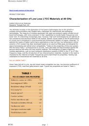
The simplest versions of common emitter and common base amplifiers are shown in the<br />
following figure. They are essentially the same amplifier with the ground connection placed on<br />
the emitter and the base respectively. The distortion output power of these two amplifiers is<br />
identical, but the concept of input referred distortion and noise power is invalid, because the<br />
source impedance is zero ohms.<br />
I out<br />
I out<br />
V S<br />
V S<br />
Fig. 1: Unmatched Undegenerated Common Emitter and Common Base LNA<br />
All real amplifier have some value for source impedance. For high frequency amplifiers, this<br />
impedance is typically provided by a low loss matching network to a 50 ohm input. The value of<br />
the source impedance seen by the amplifier is usually somewhere between the optimal value for<br />
minimum noise and maximum gain. For a typical common emitter amplifier with good<br />
performance, the desired source impedance is close to 50 ohms. For a common base amplifier<br />
the desired source impedance is much smaller than 50 ohms. The large impedance difference<br />
of a common base amplifier from 50ohms requires a high-Q matching network. High Q matching<br />
networks usually have narrower bandwidths, more in-band loss, and are more sensitivity to<br />
process variations. This will degrade the performance of the common base amplifier. The<br />
distortion performance of the matched undegenerated common emitter and common base are<br />
similar.<br />
I out<br />
I out<br />
Z S<br />
V S<br />
V S<br />
Z S<br />
Fig. 2: Matched Undegenerated Common Emitter and Common Base LNA<br />
Usually the distortion and stability performance of a undegenerated amplifier is very poor, so<br />
it is desirable to place local or global feedback around the amplifier to improve it’s performance.<br />
For a bipolar amplifer, this is easily done with some inductance in the emitter of the amplifier.<br />
This inductance also helps to make the optimal source impedance for minimum noise figure<br />
closer to the conjugate match source impedance. For a common-base it is much more difficult to<br />
linearize the amplifier, because impedances in the base have little effect on the amplifier<br />
distortion. Furthermore, inductances in the base tend to destabilize the amplifier. Incidentally,<br />
inductance in the base is an common effective way to build an oscillator, such as the Colplitt’s<br />
oscillator. Our goal here is to build an amplifier, not an oscillator, so inductance in the base is<br />
undesirable.
undesirable.<br />
Common Emitter Amplifier<br />
For the reasons of stability, low distortion, low noise, and input matching described above,<br />
an inductively degenerated common emitter configuration was chosen for the input stage of the<br />
amplifier design. The circuit is shown in the following figure. A simplified equation for the<br />
intercept point is given in the following equation [2].<br />
I out<br />
Z S<br />
V S<br />
L e<br />
Fig. 3: Matched Degenerated Common Emitter LNA<br />
IP 3ce 10<br />
10 log<br />
8I . 4. Cce ω 4 . 4<br />
L e . 1<br />
2<br />
V T<br />
I . C τ F<br />
V . T C . je0 Area<br />
2<br />
. Intercept Point of a Common-Emitter LNA<br />
Now that the first stage of the amplifier is chosen, we still have the architectural choice of<br />
adding a common base configuration (the cascode) to the output of the common emitter (the<br />
driver) configuration. This configuration is also known as a cascode configuration. The cascode<br />
configuration has the increased gain and reverse isolation advantages of all cascaded amplifiers.<br />
Unfortunately it also has the reduced dynamic range disadvantage of cascaded amplifiers from<br />
increased distortion and increased noise.<br />
When the cascode configuration is compared against two cascaded common emitter<br />
amplifiers, we see the performance is much worse. This is because first the common emitter is<br />
not matched to the common base and second because the second common base stage is not<br />
degenerated resulting in higher distortion. This disadvantage is reduced at lower frequencies as<br />
will be discussed below. If a primary goal of the amplifier was low noise and high gain it is<br />
possible to increase the performance of the amplifier with an impedance matching circuit<br />
between the common emitter and common base transistors. Unfortunately, this has the<br />
undesirable effect of reducing input referred distortion. This distortion increase comes from two<br />
different mechanisms. The first mechanism is from the increased swing at the emitter of the<br />
cascode transistor, which increases the distortion in the cascode transistor. The second<br />
mechanism comes from saturating the collector of first stage amplifier. The second mechanism<br />
can be alieviated with a higher bias for the base of the cascode transistor. In general the<br />
distortion of the cascode configuration is pretty bad without matching so it is undesirable to<br />
match the cascode and driver.<br />
An important advantage of the cascode configuration is it’s simplicity and it’s inherent bias<br />
current sharing, which shows up in cost and area comparisons. Ultimately the system requirements<br />
will justify one amplifier over another.
Common Base Amplifier<br />
To find the distortion of the cascode configuration we analyze the distortion due to the driver<br />
transistor and the cascode transistor separately. To find the distortion of the common base<br />
amplifier, we input-refer the distortion through an linear inductively degenerated transconductor.<br />
The result of the distortion from this configuration is given in the following equation.<br />
I out<br />
V S<br />
Z S<br />
V π<br />
g m*<br />
V π<br />
L e<br />
IP 3cb 10<br />
10 log<br />
Fig. 4: Common-base LNA (input-referred through ideal transconductor)<br />
4I . 3. Ccb ω . 2<br />
L e<br />
C . je0 Area . cb V T<br />
. Intercept Point of Common-Base LNA<br />
Now the distortion due to the common-emitter device can be compared to the distortion from the<br />
common base device in a cascode configuration. The following equation is result of taking the<br />
difference between the intercept point. From this difference equation we can see the common<br />
base is the dominant source of distortion at high frequencies and for large emitter degeneration.<br />
For typical values L e =1.5nH, I C =6mA, f=1.9GHz, f T =20GHz, the common emitter is 5.4dB more<br />
linear than the input referred common base. Which reduces the overall distortion of the cascode<br />
amplifier to 6.5dB below that of the common emitter alone.<br />
Intercept Point Difference between<br />
IP 3ce IP 3cb 3dB 20logg . . m ω . L e 10.<br />
log ω<br />
Common Base and Common Emitter<br />
Cascode LNA<br />
ω T<br />
V S<br />
Z S<br />
I out<br />
L e<br />
Fig. 5: Cascode LNA<br />
IP 3ce IP 3cb<br />
10 10<br />
IP 3cascode 10. log 10 10 IP 3ce 10.<br />
log 1 10<br />
∆IP 3ce_cb<br />
10<br />
Intercept Point of a Cascode LNA
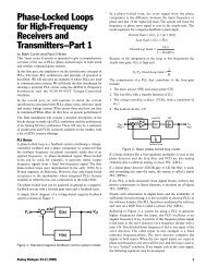
Small Signal Analysis<br />
A small signal analysis of the network is necessary for noise, gain, and impedance matching<br />
calculations. Kirkoff’s Current Laws (KCL) were used to set up a general purpose matrix to solve<br />
for the necessary gains. The following figure was used perform the small signal analysis.<br />
C µ<br />
Z S<br />
r b<br />
i bn I cn R L<br />
V S<br />
Z π<br />
g m *v π<br />
Z bias<br />
Z L<br />
v nRbias<br />
Z e<br />
v nRL<br />
Fig. 6: Small Signal Model of LNA Circuit<br />
KCL at bias node, V bias<br />
V S<br />
V bias V bias V nbias V bias V b<br />
Z S Z bias r b<br />
V S<br />
Z S<br />
V bias<br />
Z S<br />
V bias V bias V b<br />
Z bias r b<br />
KCL at base node, V b<br />
V bias V b<br />
V b V . c j. ω . C µ<br />
r b<br />
KCL at collector node, V c<br />
V b V . c j. ω . C µ g . m V b V e<br />
V b V e<br />
V b<br />
0<br />
Z π<br />
V c<br />
r o<br />
V e<br />
V c<br />
R L<br />
V c V L<br />
Z L<br />
V bias<br />
V b V . c j. ω . C µ<br />
r b<br />
V . c j. ω . C cs<br />
V b<br />
Z π<br />
V e<br />
V L<br />
V c V . b j. ω . C µ g . m V b V e<br />
Z L<br />
V c<br />
r o<br />
V e<br />
V c<br />
R L<br />
V c<br />
Z L<br />
V . c j. ω . C cs<br />
KCL at emitter node, V e<br />
V b V e<br />
g . m V b V e<br />
Z π<br />
V c<br />
r o<br />
V e<br />
V e<br />
Z e<br />
0<br />
These KCL equations are now placed into a KCL matrix<br />
V S<br />
Z S<br />
0<br />
V L<br />
Z L<br />
0<br />
1 1 1<br />
Z S Z bias r b<br />
1<br />
r b<br />
0<br />
0<br />
V e V e V b<br />
g . m V e V b<br />
Z e Z π<br />
1<br />
0<br />
0<br />
r b<br />
1<br />
j. ω . 1<br />
C µ<br />
j. ω .<br />
1<br />
C µ<br />
r b<br />
Z π<br />
Z π<br />
j. ω . C µ g m j. ω . 1 1<br />
1<br />
C µ<br />
g m<br />
Z L r o<br />
r o<br />
1<br />
1 1 1 1<br />
g m g m<br />
Z π r o Z e Z π r o<br />
Note that these equations don’t have R L in them. The necessary R L will be calculated later in the<br />
stability section.<br />
.<br />
V bias<br />
V b<br />
V c<br />
V e<br />
V e<br />
r o<br />
V c
KCL N, I C<br />
, s, Z S<br />
, Z L<br />
1 1 1<br />
Z S Z bias r b<br />
1<br />
r b<br />
0<br />
0<br />
1<br />
0<br />
0<br />
r b<br />
1<br />
j. ω . 1<br />
C µ<br />
j. ω .<br />
1<br />
C µ<br />
r b<br />
Z π<br />
Z π<br />
j. ω . C µ g m j. ω . 1 1<br />
1<br />
C µ<br />
g m<br />
Z L<br />
r o<br />
r o<br />
1<br />
1 1 1 1<br />
g m g m<br />
Z π r o Z e Z π r o<br />
KCLinv N, I C , s, Z S , Z L KCL N, I C , s, Z S , Z L<br />
1<br />
2<br />
V bias<br />
V b<br />
V c<br />
V e<br />
KCLinv N, I C , s, 50 ohm,<br />
50 ohm<br />
.<br />
50 ohm<br />
0<br />
ohm<br />
0<br />
ohm<br />
0<br />
ohm<br />
V bias 1.537 0.038i<br />
V e<br />
1.467 0.242i<br />
V b 1.498 0.03i<br />
=<br />
V c 0.129 4.151i<br />
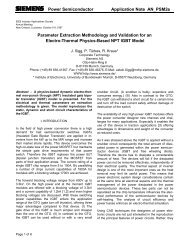
Scattering Parameter Analysis<br />
Scattering-parameters are the most widely used representation of RF small signal networks.<br />
Their advantages stem from their ease of use for power gain and reflection calculations, and<br />
serve as standard output parameters from network analyzers. S parameter values can be<br />
calculated for a small signal network using a variety of procedures including calculating other<br />
parameters and converting to S parameters, but the following method is chosen for it’s simplicity.<br />
The S parameters are referenced to 50 ohms, because it a common value used in test<br />
equipment, passive components, such as filters and antennas, and commercially available active<br />
components, such as amplifiers and mixers.
2V<br />
50 Ω<br />
1V<br />
1 GΩ<br />
S 21<br />
Circuit<br />
S 11<br />
50 Ω<br />
S 12<br />
50 Ω<br />
50 Ω<br />
Circuit<br />
1V<br />
2V<br />
S 22<br />
1 GΩ<br />
Fig. 7: Circuit used for scattering parameter calculations<br />
2<br />
50 ohm<br />
0<br />
Sparam N, I C , s V KCLinv N, I C , s, 50 ohm,<br />
50 ohm .<br />
ohm<br />
0<br />
ohm<br />
0<br />
ohm<br />
S 11 ,<br />
V 1<br />
1<br />
S 21 ,<br />
V 3<br />
V<br />
KCLinv N, I C , s, 50 ohm,<br />
50 ohm<br />
S 22 ,<br />
V 3<br />
1<br />
S 12 ,<br />
V 1<br />
S<br />
.<br />
0<br />
ohm<br />
0<br />
ohm<br />
2<br />
50 ohm<br />
0<br />
ohm<br />
Sparam N, I C , s<br />
=<br />
0.537 0.038i<br />
0.129 4.151i<br />
0.015 0.098i<br />
0.648 0.278i
100<br />
10<br />
1<br />
0.1<br />
0.01<br />
0.01 0.1 1 10 100<br />
| S11 |<br />
| S21 |<br />
| S12 |<br />
| S22 |<br />
Fig. 8: S Parameters vs. Frequency<br />
Stability Analysis<br />
Often it happens a designer designs an amplifier, but he gets an oscillator in return. This<br />
scenario typically occurs at frequencies out of the desired band, where the source and load<br />
impedances can be unknown. If the out of band source and load impedances are unknown it is<br />
desirable to make the amplifier stable for all source and load impedances. This is known as an<br />
unconditionaly stable amplifier. If the out-of-band source and load impedances are known it is<br />
possible to design a conditionally stable amplifier design. Usually conditionally stable amplifiers<br />
can acheive higher performance levels than unconditionally stable amplifiers. This is becuase<br />
the amplifier performance must be degraded some with form of ballasting resistor to make it<br />
stable.<br />
It is desirable to make the stability factor greater than one for another reason other than<br />
stability. With a K factor greater than one it is possible to simultaneously conjugate match the<br />
input and output impedance of the amplifier. Conjugate matches are desirable, because the<br />
filters connected to the amplifier require a conjugate impedance to provide their specified<br />
frequency response.<br />
For a K factor of one, the real part of the matching impedances is zero ohms, so it is<br />
impossible to match with practical matching networks. For this same reason it is desirable to<br />
make the K factor some value significantly larger than one.<br />
KS ( ) ∆ S .<br />
1, 1<br />
S 22 ,<br />
S .<br />
12<br />
,<br />
S 2,<br />
1<br />
1 ( ∆ ) 2 2<br />
S 1, 1<br />
2. S .<br />
1,<br />
2<br />
S 21 ,<br />
2<br />
S 2, 2<br />
K Sparam N, I C , s = 1.016<br />
The mu factor is often a more desirable parameter to use for stability than K factor. This is<br />
because the K factor must be specified with other conditions, such as ∆. In this sense the µ<br />
factor is easier to use, because it does not require any other parameters to guarantee<br />
unconditional stability. Although the K factor and µ factor curves are different, their values are<br />
equal for the transition point between unconditionally stable and conditionally stable regions<br />
(K=µ=1). µ S<br />
.<br />
, , s = 1.102<br />
( ) ∆ S .<br />
1, 1<br />
S 22 ,<br />
S 12<br />
S 1 1<br />
,<br />
S 2,<br />
1<br />
2<br />
1 S 22 ,<br />
,<br />
∆ . S 2,<br />
2<br />
S .<br />
2 1<br />
,<br />
S 12 ,<br />
µ Sparam N I C
10<br />
1<br />
K, Mu<br />
0.1<br />
0.01<br />
0.01 0.1 1 10 100<br />
K Factor<br />
mu Factor<br />
Desired Stability Factor<br />
Frequency<br />
Fig. 9: K Stability Factor vs. Frequency<br />
1.15<br />
1<br />
K, Mu<br />
1.1<br />
K, Mu<br />
0.8<br />
1.05<br />
0.6<br />
1<br />
0 20 40 60 80 100<br />
0.4<br />
0 5 10 15 20<br />
Number of Device in Parallel<br />
K Factor<br />
Mu Factor<br />
Desired Stability Factor<br />
Bias Current (mA)<br />
K Factor<br />
Mu Factor<br />
Desired Stability Factor<br />
Fig. 10: K Factor vs. Device Size<br />
Fig. 11: K Factor vs. Bias Current
Ballast Resistor Sizing<br />
The term ballast is of Swedish origin, where bal means " to bear," and llast means "load."<br />
Thus the term ballast means to bear the load. The load refers to a heavy weight placed at the<br />
bottom of ship to stabilize the ship in heavy waves. The term ballast is used here to describe a<br />
resistor, which is added to the circuit to provide stability. Most transistors given by a<br />
manufacturer are only conditionally stable. For this reason, and the reasons described above a<br />
ballast resistor is added to stabilize the transistor<br />
The following procedure is used to find the ballast resistor needed to make the amplifier<br />
unconditionally stable, or to provide the desired K factor. First, the procedure involves<br />
converting a given set of S parameters to ABCD parameters and multiplying them with the S<br />
parameters of a parallel resistor. Then the combination ABCD parameters are converted back<br />
into a new set of S parameters, which are used to find the K factor for the device. The value of<br />
resistance is swept to find the value need to meet a desired value of K factor.<br />
ABCD Parameters of a Parallel Resistor<br />
ABCD( R)<br />
1<br />
ohm<br />
R<br />
0<br />
1<br />
S to ABCD Parameter Calculation<br />
S2ABCD S,<br />
Z 0<br />
Note: The units are removed, for calculation purposes only<br />
1 S .<br />
1, 1<br />
1 S 22 ,<br />
S .<br />
12<br />
.<br />
2S 2,<br />
1<br />
,<br />
S 2,<br />
1<br />
ohm 1 S .<br />
1, 1<br />
1 S 22 ,<br />
S .<br />
.<br />
12<br />
Z .<br />
0<br />
2S 21 ,<br />
,<br />
S 21 ,<br />
Z 0 1 S .<br />
1, 1<br />
1 S 22 ,<br />
S .<br />
.<br />
12<br />
ohm<br />
.<br />
2S 21 ,<br />
1 S .<br />
1, 1<br />
1 S 22 ,<br />
S .<br />
12<br />
.<br />
2S 2,<br />
1<br />
,<br />
S 21 ,<br />
,<br />
S 2,<br />
1<br />
S2ABCD Sparam N, I C , s , 50 ohm<br />
=<br />
0.063 0.013i<br />
1.39. 10 4 1.384i . 10 3<br />
2.099 17.814i<br />
0.013 0.042i<br />
ABCD to S Parameter Calculation<br />
ABCD2S ABCD, Z 0 A ABCD 11 ,<br />
B ABCD 12 ,<br />
C ABCD 21 ,<br />
A<br />
D ABCD 22 ,<br />
1<br />
B . ohm<br />
Z 0<br />
Z 0<br />
C. D<br />
ohm<br />
.<br />
A<br />
B . ohm C. Z 0<br />
D<br />
Z 0 ohm<br />
2<br />
A<br />
2.( A. D BC . )<br />
B . ohm<br />
Z 0<br />
Z 0<br />
C. D<br />
ohm<br />
ABCD2S S2ABCD Sparam N, I C , s , 50 ohm , 50 ohm<br />
=<br />
0.537 0.038i<br />
0.129 4.151i<br />
1 0<br />
KwithR( S,<br />
R) K ABCD2S S2ABCD( S,<br />
50 ohm)<br />
. ohm ,<br />
1<br />
50 ohm<br />
R<br />
0.015 0.098i<br />
0.648 0.278i<br />
K Factor with Load Resistor<br />
KwithR Sparam N , I C , s , 1000 ohm = 1.082
1 0<br />
µwithR( S,<br />
R) µ ABCD2S S2ABCD( S,<br />
50 ohm)<br />
. ohm ,<br />
1<br />
50 ohm<br />
R<br />
µwithR Sparam N , I C<br />
, s , 1000 ohm = 1.248<br />
µ Factor with Load Resistor<br />
1.3<br />
K and Mu Factor<br />
1.2<br />
1.1<br />
1<br />
100 1 .10 3 1 .10 4<br />
Ballast Resistance (kohm)<br />
K Factor<br />
Mu Factor<br />
Desired K Factor<br />
Fig. 12: K and Mu vs. Ballast Resistor<br />
Rguess<br />
0.1 kΩ<br />
Rneeded N , I C , s, Kval if K Sparam N, I C , s > Kval, 100 kΩ,<br />
root KwithR Sparam N, I C , s , Rguess Kval,<br />
Rguess<br />
Rneeded2 N , I C , s, Kval if µ Sparam N , I C , s > Kval, 100 kΩ,<br />
root µwithR Sparam N, I C , s , Rguess Kval,<br />
Rguess<br />
Rneeded2 N , I C , s, K val = 100 kΩ<br />
R L N, I C , s Rneeded N, I C , s, K val R L N, I C , s = 773.703 ohm<br />
It is interesting to plot the ballast resistor needed vs. the device size and current. These<br />
curves are shown in the following figures. From these plots we see the stability of the device<br />
increases with bias current and decreases with device size. Conversely we see we need a<br />
smaller parallel ballast resistor for more potentially unstable devices. Thus a smaller ballast<br />
resistor is needed for larger devices and devices with smaller currents.<br />
1 .10 6 Ballast Resistor Need to make K=Kval<br />
Ballast Resistor Size (ohms)<br />
1 .10 5<br />
1 .10 4<br />
1 .10 3<br />
100<br />
1 10 100<br />
Number of Devices in Parallel<br />
Ballast Resistor Need to make mu=Kval<br />
Fig 13: Ballast Resistor vs. Device Size
2000<br />
Ballast Resistor (ohms)<br />
1500<br />
1000<br />
500<br />
0<br />
0 5 10 15 20<br />
Resistance Needed w/ 25 Devices<br />
Resistance Needed w/ 50 Devices<br />
Resistance Needed w/ 75 Devices<br />
Bias Current (mA)<br />
Fig. 14: Ballast Resistor vs Current<br />
Simultaneous Conjugate Matching Analysis<br />
It is desirable from a gain perspective to simultaneously conjugate the input and output of the<br />
amplifier. This maximizes gain, but may not be optimal for noise as we shall see later. If the<br />
device is unilateral (i.e. the reverse isolation, S12, is zero) the conjugate matching impedances<br />
can be calculated directly from S11 and S22. In reality S12 is some non-zero value, so matching<br />
the input will change the impedance at the output. Simultaneous matching can be done<br />
iteratively, which can be tedious and time consuming. An easier method involves solving a<br />
second order equation for the desired values. The derivation of Zpopt is done in [4]. To use the<br />
equation the S-Parameters must first be recalculated with the necessary ballast resistor.<br />
KCL N, I C , s, Z S , Z L<br />
1 1 1<br />
Z S Z bias r b<br />
1<br />
r b<br />
0<br />
0<br />
1<br />
0<br />
0<br />
r b<br />
1<br />
j. ω . 1<br />
C µ<br />
j. ω .<br />
1<br />
C µ<br />
r b<br />
Z π<br />
Z π<br />
j. ω . C µ g m j. ω . 1 1 1<br />
1<br />
C µ<br />
g m<br />
R L Z L r o<br />
r o<br />
1<br />
1<br />
1 1 1<br />
g m g m<br />
Z π r o Z e Z π r o<br />
KCLinv N, I C , s, Z S , Z L KCL N, I C , s, Z S , Z L<br />
1
Sparam N, I C<br />
, s KCLi KCLinv N , I C<br />
, s, 50 ohm,<br />
50 ohm<br />
V<br />
KCLi.<br />
S 11 ,<br />
V 1<br />
1<br />
S 21 ,<br />
V 3<br />
V<br />
KCLi.<br />
S 22 ,<br />
V 3<br />
1<br />
S 12 ,<br />
V 1<br />
S<br />
2<br />
50 ohm<br />
0<br />
ohm<br />
0<br />
ohm<br />
0<br />
ohm<br />
0<br />
ohm<br />
0<br />
ohm<br />
2<br />
50 ohm<br />
0<br />
ohm<br />
Sparam N, I C , s<br />
=<br />
0.548 0.015i<br />
0.256 3.975i<br />
5.547 . 10 3 0.095i<br />
0.599 0.115i
Z popt SZ , 0 ∆ S .<br />
11 ,<br />
S 22 ,<br />
S .<br />
1 2<br />
2<br />
B 1 1 S 11 ,<br />
2<br />
B 2 1 S 22 ,<br />
,<br />
S 21 ,<br />
2<br />
S 22 ,<br />
2<br />
S 11 ,<br />
( ∆ ) 2<br />
( ∆ ) 2<br />
C 1 S 11 ,<br />
∆ . S 22 ,<br />
C 2 S 22 ,<br />
∆ . S 11 ,<br />
Γ Spopt<br />
B 1 B 1<br />
2<br />
2C . 1<br />
4.<br />
2<br />
C 1<br />
2<br />
B 1 B 1<br />
Γ Spopt if Γ Spopt < 1,<br />
Γ Spopt ,<br />
Γ Lpopt<br />
B 2 B 2<br />
2<br />
2C . 2<br />
4.<br />
2<br />
C 2<br />
2<br />
B 2 B 2<br />
Γ Lpopt if Γ Lpopt < 1,<br />
Γ Lpopt ,<br />
1 Γ<br />
Z Lpopt Z . Lpopt<br />
0<br />
1 Γ Lpopt<br />
1 Γ<br />
Z Spopt Z . Spopt<br />
0<br />
1 Γ Spopt<br />
Z Spopt<br />
2C . 1<br />
2C . 2<br />
4.<br />
2<br />
C 1<br />
4.<br />
2<br />
C 2<br />
Z Lpopt<br />
Z L N, I C , s Z popt Sparam N, I C , s , 50 ohm<br />
Z Sp N, I C , s Z popt Sparam N, I C , s , 50 ohm<br />
2<br />
1<br />
Z L N, I C , s = 120.278 52.473i ohmOptimal Load Impedance<br />
Z Sp N, I C , s = 91.811 18.536i ohmOptimal Source Impedance<br />
1 .10 3 Fig. 14: Max Gain Impedaces vs Frequency<br />
Impedance (ohms)<br />
100<br />
10<br />
0.1 1 10 100<br />
Frequency (GHz)
Noise Analysis<br />
Noise analysis for low noise amplifier design is important not only for the definition of the<br />
amplifier, but also for it’s application. The noise requirements are determined by the amplitude<br />
of the signal being received and the desired signal to noise ratio. It is also important to allow<br />
some of the total system noise budget to other elements in the receiver chain. For cellular<br />
phones the desired signal amplitude is calculated when the cellular phone is the farthest<br />
distance from the base station.<br />
To do the noise calculation we need to include all of the noise sources for the entire low noise<br />
amplifier circuit, including noise from the bias circuitry and ballast resistor. To simplify the bias<br />
noise calculations we first need to convert the bias circuit into an equivalent parallel resistance<br />
and inductance. The current noise from this parallel resistor is added to the input referred current<br />
noise of the amplifier and not in the input referred voltage noise. In reality it will also have a small<br />
affect on the voltage noise, but since the bias impedance is usually large it is acceptable to model<br />
the noise as a current source.<br />
Conversion from Z bias to L bias and R bias<br />
Im Z bias<br />
Q bias<br />
Q bias = 5.969 Q of an L S in series with R S<br />
Re Z bias<br />
2<br />
L bias if Q bias 0,<br />
j10 . 9 1 Q bias Im Z bias<br />
H, .<br />
L<br />
2<br />
bias 51.403 nH<br />
Q ω<br />
bias<br />
= Equivalent Parallel Inductance<br />
R bias 1 Q bias<br />
2<br />
. Re Z bias<br />
R bias 3.663 . 10 3 ohm<br />
= Equivalent Parallel Bias Resistance<br />
To simplify the noise analysis we neglect C µ . C µ is only important for stability and gain analysis.<br />
KCL analysis of the simplified circuit with noise sources is used to find the gains of the noise<br />
sources.<br />
at Base Node<br />
V s V b V b V e<br />
V s V b V b V e<br />
i bn<br />
r b Z S Z π r b Z S r b Z S Z π<br />
at Emitter Node<br />
V b V e<br />
V<br />
i bn g . e<br />
m V b V e i cn 0<br />
Z π Z e<br />
at Collector Node<br />
V b V e<br />
g . m V b V e<br />
Z π<br />
V<br />
g . c<br />
m V b V e i cn 0 0 g . m V b V e<br />
Z L<br />
V c<br />
Z L<br />
V e<br />
Z e<br />
KCLsimpleinv Z S , Z L<br />
1<br />
1<br />
0<br />
r b ( N) Z S Z π N, I C , s<br />
1<br />
g m I C<br />
Z L<br />
1<br />
g m I C 0<br />
Z π N, I C , s<br />
1<br />
Z π N, I C , s<br />
1<br />
Z π N, I C , s<br />
g m I C<br />
1<br />
g m I C<br />
Z e ( N,<br />
s)<br />
1<br />
79.793 13.307i<br />
0<br />
0.301 3.141i<br />
KCLsimpleinv Z Sp N, I C , s , Z L N, I C , s<br />
=<br />
377.04 445.504i<br />
120.278 52.473i<br />
94.09 50.208i<br />
ohm<br />
76.496 24.317i<br />
0<br />
1.793 3.307i
Solve<br />
r . b i . bn Z . e β β . V . s Z e Z . S i . bn Z . e β i . bn Z . π Z S i . bn Z . π r b Z . π V s Z . S i . cn Z e V . s Z e r . b i . cn Z e<br />
Z S r b g . m Z . π Z e Z e Z π<br />
Z . L<br />
Z . S i . bn Z . π g m r . b i . bn Z . π g m Z . π V . s g m i . bn Z . π Z . e g m Z . S i cn r . b i cn i . cn Z e i . cn Z π<br />
Z S r b g . m Z . π Z e Z e Z π<br />
A v<br />
Z . e<br />
i . cn Z π r . b i cn i . bn Z π Z . S i . bn Z . π g m r . b i . bn Z . π g m Z . π V . s g m Z . S i cn V s<br />
β N, I C , s . para R L N, I C , s , Z L N, I C , s<br />
r b ( N) β N, I C , s 1 . Z e ( N,<br />
s)<br />
Z π N, I C , s<br />
Z S r b g . m Z . π Z e Z e Z π<br />
A v = 2.845 5.479i Zero Source Impedance<br />
Voltage Gain<br />
A i β N, I C , s . para R L N, I C , s , Z L N, I C , s A i = 1.438 2.475i kΩ Infinite Source Impedance<br />
Current Gain<br />
Now we can use the gains we just calculated to find the equivalent input voltage and current<br />
sources and the correlation between the two. In order to find the equivalent input noise source,<br />
we must first know the magnitude of each of the individual noise sources. These are well known<br />
values of 4kTr b for the base resistance thermal noise, 2qI B for the base current shot noise, and<br />
2qI C for the collector current shot noise.<br />
v bn ( N ) 4. k. Temp. r b ( N)<br />
v bn N = Base Thermal Noise Voltage<br />
( ) 0.271 nV Hz<br />
i cn I C<br />
i bn I C<br />
2q . . I C<br />
2q .<br />
I<br />
. C<br />
β 0<br />
i cn I C = 56.604 pA Collector Shot Noise Current<br />
Hz<br />
i bn I C = 4.682 pA Base Shot Noise Current<br />
Hz<br />
i biasn R bias<br />
i RLn R L<br />
4k . . 1<br />
Temp. i biasn R bias 2.126 pA<br />
R bias<br />
Hz<br />
4k . . 1<br />
Temp. i RLn R L 4.626 pA<br />
R L N, I C , s<br />
Hz<br />
= Bias Resistor Current Noise<br />
= Load Resistor Current Noise
Equivalent Input Noise Elements<br />
The equivalent input-referred voltage noise source is found by setting the source impedance<br />
to zero, finding the transfer function of all the noise sources to the output, adding the up all the<br />
noise powers at the output, and dividing by the voltage gain from the source itself. Similarly,<br />
the equivalent input-referred current noise can be found with an input current source and the<br />
source impedance set to infinity.<br />
Noiseless<br />
Noiseless<br />
v n<br />
Z L<br />
Z L<br />
i neq<br />
Fig. 15: Circuit used to find input-referred noise voltage<br />
Fig. 16: Circuit used to find input-referred noise current<br />
V neq N, I C , s 4k . . Temp. r b ( N ) r b ( N) Z e ( N,<br />
s)<br />
+<br />
r b ( N) Z e ( N,<br />
s) Z π N, I C , s<br />
β N, I C , s<br />
4k . . 1<br />
+ Temp.<br />
.<br />
R L N, I C , s<br />
2 2<br />
. . q.<br />
I B I C<br />
2<br />
. 2 . q.<br />
I C ...<br />
r b ( N ) β N, I C , s 1 . Z e ( N,<br />
s)<br />
Z π N, I C , s<br />
...<br />
β N, I C , s<br />
2<br />
I neq N, I C , s 4k . . Temp<br />
2q . . I B I C<br />
R bias<br />
V neq N, I C , s = 0.317 nV Equivalent Input Noise<br />
Hz<br />
Voltage<br />
2q . . I C 4k . . 1<br />
Temp.<br />
R L N, I C , s<br />
β N, I C , ω<br />
2<br />
Equivalent Input Noise<br />
Current<br />
I neq N, I C , s = 5.764 pA Hz<br />
The input referred noise can be represented by two noise resistances and the correlation<br />
impedance or admittance. R n is the value of a resistor whose voltage thermal noise is equal to<br />
the equivalent input voltage noise. g n is the value of a resistor whose current thermal noise is<br />
equal to the equivalent input current noise.<br />
R n N, I C , s<br />
g n N, I C , s<br />
2<br />
V neq N, I C , s<br />
4k . . Temp<br />
2<br />
I neq N, I C , s<br />
4k . . Temp<br />
R n N, I C , s = 6.064 Ω Equivalent Input Noise<br />
Resistance<br />
1<br />
g n N, I C , s<br />
498.381 Ω<br />
= Equivalent Input Noise<br />
Conductance
Noise Correlation<br />
Except in special cases, the optimal noise source impedance will be different from the optimal<br />
power source impedance. Thus, when using the optimal noise source impedance, the power<br />
gain will not be maximized. On the other hand lower power gain will increase the significance of<br />
the noise from later stages on the noise figure of the system. Thus a tradeoff exists between the<br />
optimal noise source impedance and optimal power source impedance for minimum overall<br />
system noise figure. The optimal source impedance for minimum system noise figure can be<br />
found by including the noise of the following stages, such as the mixer, in the optimal noise<br />
source impedance calculation. In many optimal source impedance calculations, other sources of<br />
noise are also neglected. The noise sources to be included in the source impedance calculation<br />
are noise from the bias source, bonding pad series resistance, series resistance of inductor<br />
degeneration from bond wires and especially from low-Q on-chip spiral inductors. The series<br />
resistance of these spirals tend to increase optimal noise source impedance, when they are used<br />
for emitter degneration of common emitter and common source amplifiers.<br />
To find the noise gains, a load impedance is assumed, which will in turn affect the gains and the<br />
optimal noise source impedance. The optimal load impedance for maximum power transfer is a<br />
good guess for the load impedance. It becomes a better guess as the noise of following stages is<br />
increased. Once the optimal source impedance is found using a guess for the load impedance, the<br />
load impedance for maximum power transfer should be recalculated from the complex conjugate of<br />
the output impedance of the device with the optimal system noise source impedance.<br />
Thus the steps for finding optimal system noise source impedance are as follows:<br />
1. Find S parameters of the circuit directly or indirectly by finding the Y<br />
parameters of the device directly.<br />
2. Find the optimal load and source impedance with the calculated S<br />
parameters.<br />
3. Find the gains of all noise sources and an input voltage source to the output<br />
with a zero source impedance. Include all noise source gains, including the<br />
noise of following stages and bias noise.<br />
4. Find the gains of all noise sources and an input current source to the output<br />
with a infinite source impedance.<br />
5. Use the gains to find the input referred equivalent voltage and noise sources<br />
and the correlation impedance.<br />
6. Use the equivalent voltage and current noise sources to find the equivalent<br />
series and parallel noise resistances.<br />
7. Use the correlation impedance and noise resistances to find the optimal<br />
source impedance.<br />
8. Recalculate desired output impedance given the optimal system noise<br />
source impedance.<br />
.<br />
I<br />
VI conj N, I C , s r b ( N) Z e ( N,<br />
s) . 2.<br />
C<br />
q. r b ( N ) Z e ( N,<br />
s) Z π N, I C , s<br />
β 0<br />
+<br />
VI conj N, I C , s = 0 W Hz<br />
r b ( N ) β N, I C , s 1 . Z e ( N,<br />
s)<br />
Z π N, I C , s<br />
.<br />
2q . I C<br />
β N, I C , s<br />
4k . . 1<br />
Temp.<br />
R L N, I C , s<br />
.<br />
β N, I C , s<br />
2<br />
2<br />
...
γ N, I C<br />
, s<br />
VI conj N, I C<br />
, s<br />
V neq N, I C<br />
, s<br />
2.<br />
I neq N, I C<br />
, s<br />
2<br />
γ N, I C<br />
, s = 0.111 0.088i<br />
Correlation Coefficient<br />
The correlation impedance is derived from the zero and infinite source impedance noise<br />
gains and the equivalent input noise sources. The noise correlation impedance is useful for<br />
finding the optimal source impedance for low noise. In the special case, where the input<br />
equivalent voltage and noise sources are 100% correlated, the correlation impedance is equal to<br />
the input impedance. This ideal scenario allows maximum power transfer to occur<br />
simultaneously with minimum noise figure. An example when this situation occurs is when the<br />
backend noise, such as the mixer noise, is high.<br />
The correlation impedance or admittance between the input equivalent current and voltage<br />
noise can now be calculated as shown in the following equations. Note that the correlation is not<br />
equal to the inverse of the correlation impedance, except in the special case, where current and<br />
voltage noise is 100% correlated.<br />
Noiseless<br />
Noiseless<br />
Z S<br />
v n<br />
i n<br />
Z L<br />
Z S<br />
v neq<br />
i n2<br />
=Y corr<br />
*V neq<br />
Z L<br />
i n1<br />
Fig. 17: Circuit with correlated noise sources<br />
Fig. 18: Circuit used to find Y corr<br />
Y corr N, I C , s γ N, I C , s<br />
I neq N, I C , s<br />
. 1<br />
2<br />
V neq N, I C , s<br />
2<br />
Y corr N, I C , s<br />
= 304.9 241.319i Ω Correlation Conductance<br />
Noiseless<br />
v n2<br />
=Z corr<br />
*I neq<br />
Z S<br />
v n1<br />
i neq<br />
Z L<br />
Fig. 19: Circuit used to find Z corr<br />
Z corr N, I C , s γ N, I C , s<br />
2<br />
V neq N, I C , s<br />
. Z<br />
2 corr N, I C , s 6.094 4.823i Ω<br />
I neq N, I C , s<br />
= Correlation Impedance
n is the noise resistance representing the portion of V neq<br />
2 which is uncorrelated with I neq<br />
2.<br />
It is always less than R n , and in the case where the noise is 100% correlated, it is equal to 0.<br />
r n N, I C<br />
, s R n N, I C<br />
, s . 1 γ N, I C<br />
, s r n N, I C<br />
, s 5.943 Ω<br />
2<br />
= Correlation Resistance<br />
G n is the noise resistance representing the portion of I 2 neq which is uncorrelated with V neq<br />
2.<br />
It is always greater than g n , and in the case where the noise is 100% correlated, it is equal to<br />
infinity.<br />
2<br />
G n N, I C<br />
, s g n N, I C<br />
, s . 1 γ N, I C<br />
, s<br />
1<br />
G n N, I C , s<br />
Optimal Noise Figure and Source Impedance<br />
= 508.546 Ω Correlation Conductance<br />
The optimal source resistance is then given by the following equation, using admittance or<br />
impedance noise parameters. Both cases should given the same answer.<br />
Z nopt N, I C , s<br />
r n N, I C , s<br />
g n N, I C , s<br />
Z nopt N, I C , s = 54.761 4.823i ohm<br />
Re Z corr N, I C , s<br />
2<br />
. Optimal Source Impedance<br />
for Minimal Noise Figure<br />
jImZ corr N, I C , s<br />
In the special case, where the noise of the following stages dominates, the optimal noise<br />
source impedance will equal the optimal power source impedance. In the special case, where the<br />
noise of the following stages is zero, the optimal system source impedance will equal the optimal<br />
device source impedance. An optimal system noise figure can be derived by cascading an<br />
infinite number of identical devices and finding the optimal source impedance. Friis explored this<br />
ideal to derive and optimal system source impedance given a single device charateristics. In<br />
reality, all of the devices in a receiver chain will not be the same for distortion purposes.<br />
NF min N, I C , s 10.<br />
log 1 2.<br />
g n N, I C , s . Re Z corr N, I C , s<br />
...<br />
+<br />
g n N, I C , s . r n N, I C , s g n N, I C , s Re Z corr N, I C , s<br />
.<br />
2<br />
NF min N, I C , s = 0.949 dB<br />
Optimal Noise Figure<br />
Noise figure will also be increased by a jammer a frequency offset from the desired signal<br />
f off +f desired , mixing with bias noise at the same offset at basband, f off . This derivation is breifly<br />
described in the <strong>Mathcad</strong> file: biasnoise.mcd.
Noise Figure Plots<br />
NF N, I C<br />
, s, Z S 10.<br />
log 1<br />
r n N, I C<br />
, s<br />
Re Z S<br />
g n N, I C<br />
, s<br />
. Z S Z corr N, I C<br />
, s<br />
Re Z S<br />
2<br />
4<br />
5<br />
3<br />
4<br />
Noise Figure (dB)<br />
2<br />
Noise Figure (dB)<br />
3<br />
2<br />
1<br />
1<br />
0<br />
0 200 400 600<br />
0<br />
200 100 0 100 200<br />
Source Resistance (ohms)<br />
Source Reactance (ohms)<br />
Fig. 20:Noise Figure vs Source Impedance<br />
Fig. 21:Noise Figure vs Source Reactance<br />
1.4<br />
2.5<br />
Minimum Noise Figure (dB)<br />
1.2<br />
1<br />
0.8<br />
Minimum Noise Figure (dB)<br />
2<br />
1.5<br />
1<br />
0.6<br />
0 5 10 15 20<br />
0.5<br />
0 20 40 60 80 100<br />
Bias Current (mA)<br />
Minimum Noise Figure (dB)<br />
Number of Devices in Parallel<br />
Minimum Noise Figure (dB)<br />
Fig. 22: Min. Noise Figure vs. Current<br />
Fig. 23: Noise Figure vs. Device Size<br />
150<br />
150<br />
100<br />
100<br />
Impedance (ohms)<br />
50<br />
Impedance (ohms)<br />
50<br />
0<br />
0<br />
50<br />
0 5 10 15 20<br />
50<br />
0 20 40 60 80 100<br />
Bias Current (mA)<br />
Imaginary Part of Optimal Source Impedance<br />
Real Part of Optimal Source Impedance<br />
Number of Devices in Parallel<br />
Imaginary Part of Optimal Source Impedance<br />
Real Part of Optimal Source Impedance<br />
Fig 24: Optimal Noise Impedance vs Ibias<br />
Fig. 25:Optimal Source Impedance vs Size
Optimal Source Impedance to Trade-Off Power and Noise<br />
The following method is a crude, but quick and relatively easy method for finding the optimal<br />
source impedance to trade-off power and noise. A more accurate method is discusses below<br />
but not implemented.<br />
Optimal Noise Source Impedance:<br />
Z n =r n +jx n ,<br />
NF=NF min<br />
Optimal Gain Source Impedance<br />
Z p =r p +jx p ,<br />
G=G max ,<br />
S 11 =0<br />
Constant S 11 contour<br />
Desired Source Impedance<br />
Z=r+jx<br />
S 11 =Desired Specification<br />
Fig. 26: Figure used to illustrade noise and power trade-off<br />
In the design of a low noise amplifier,LNA, or mixer driver stage there exists an optimal source<br />
source impedance to provide the maximum power transfer into the transistor and thus the<br />
maximum gain. There also exists an optimal source impedance, Z nopt , to provide the minimum<br />
noise figure for the circuit. At the maximum power source impedance, Z popt , the input is matched<br />
to the source impedance and no reflections occur. This is desirable, because the filters attached<br />
to designed for the LNA or mixer, are designed for a matched load impedance, but can tolerate a<br />
certain amount of deviation from it’s desired impedance. The amount of acceptable deviation is<br />
usually specified by the maximum return loss, or S 11 , the filter can handle. The routine below<br />
finds the source impedance to the LNA or mixer, which will provide the lowest noise figure and<br />
maximum gain, while maintaining a desired S 11 specification.<br />
The calculation is performed by drawing a straight line between the optimal noise and power<br />
source impedances and finding where it intersects the desired S 11 contour. This line intersects<br />
the contour at two points, so the point must be chosen, which is closet to the optimal noise<br />
source impedance. Sometimes, the desired S 11 specification is acheived at the optimal noise<br />
source impedance. In this case the optimal noise source impedance is chosen over the<br />
intersecting point. This calculation is not optimal in the truest sense, because the noise and<br />
power gain circles are not coencentric, but it serves as an good estimate to meet design criteria.
Z Ss11 Z p<br />
, Z n<br />
, S 11goaldB S 11goal 10<br />
S 11goaldB<br />
20<br />
Z in<br />
r i<br />
x i<br />
r p<br />
x p<br />
r n<br />
x n<br />
Z p<br />
Re Z in<br />
Im Z in<br />
Re Z p<br />
Im Z p<br />
Re Z n<br />
Im Z n<br />
S 11n 20 log Z in Z<br />
.<br />
n<br />
Z in Z n<br />
g<br />
1 S 11goal<br />
2<br />
1 S 11goal<br />
2<br />
m x p x n<br />
r p r n<br />
a 1 m 2<br />
b 2. x i x n mr . . n m 2r . . i g<br />
c r i<br />
2<br />
x i x n mr . 2<br />
n<br />
1<br />
r . 1<br />
( 2a . )<br />
b b 2 4a . . c<br />
x 1 m. r 1 r n x n<br />
d 1 r 1 r n<br />
2<br />
x 1 x n<br />
2<br />
1<br />
r . 2<br />
( 2a . )<br />
b b 2 4a . . c<br />
x 2 m. r 2 r n x n<br />
d 2 r 2 r n<br />
2<br />
x 2 x n<br />
2<br />
r if d 1 < d 2 , r 1 , r 2<br />
x if d 1 < d 2 , x 1 , x 2<br />
Z Sans<br />
if S 11n < S 11goaldB , Z n , r 1.<br />
x<br />
Z Sans<br />
Z Sp N, I C , s = 91.811 18.536i ohm<br />
Optimal Source Impedance for Conjugate Matching<br />
Z nopt N, I C , s = 54.761 4.823i ohm<br />
Optimal Source Impedance for Minimum Noise Figure<br />
Z S N, I C , s Z Ss11 Z Sp N, I C , s , Z nopt N, I C , s , S 11goaldB Z S N, I C , s = 67.707 3.339i ohm<br />
Optimal Source Impedance to trade-off Noise and<br />
Power
Gain Analysis<br />
Z2Γ( Z)<br />
Z<br />
Z<br />
G T<br />
Γ G<br />
, Γ L<br />
, S<br />
50 ohm<br />
50 ohm<br />
Available Power Gain<br />
1 Γ L<br />
2<br />
2<br />
S 2, 1<br />
Power<br />
2<br />
. . 1 Γ G<br />
1 S .<br />
22 ,<br />
Γ . L<br />
1 S .<br />
1, 1<br />
Γ G S 12<br />
Impedance to Reflection Coefficient Conversion<br />
. . Γ L<br />
Γ G<br />
,<br />
S 21 ,<br />
.<br />
2<br />
Transducer Gain<br />
G avail N, I C<br />
, s 10. log G T Z2Γ Z S N, I C<br />
, s , Z2Γ Z L N, I C<br />
, s , Sparam N, I C<br />
, s G avail N, I C<br />
, s = 14.166 dB<br />
15<br />
25<br />
Available Power Gain (dB)<br />
14<br />
13<br />
Available Power Gain (dB)<br />
20<br />
15<br />
12<br />
0 5 10 15 20<br />
10<br />
0 20 40 60 80 100<br />
Bias Current (mA)<br />
Available Power Gain (dB)<br />
Number of Devices in Parallel<br />
Available Power Gain (dB)<br />
Fig. 27: Power Gain vs. Bias Current<br />
Fig. 28: Power Gain vs. Device Size<br />
Distortion Analysis<br />
The distortion analysis routines were copied directly from the thesis of Keng Fong [2]. They are<br />
the most inaccurate portion of the design routine as they do not reflect the impact of the input<br />
matching network on distortion performance. From comparisions to simulations we see the results<br />
differ by 3-9dB. Future work will add the effects of the input matching network and bias circuitry.<br />
Low distortion in a low noise amplifier is important to prevent undesired signals from<br />
interfering with the desired signal. The most important measure of distortion performance is the<br />
third order intercept point. The scenario where third order distortion is important is when the<br />
receiving device is located a distance far from the transmitting device, and two devices are<br />
transmitting signals close to the device, spacing at frequencies ∆f and 2*∆f from the desired<br />
signal. Through third order distortion, the undesired signals, jammers, mix together to produce a<br />
signal in the desired band. To prevent this signal from degradation the performance of the<br />
receiver the low noise amplifier must be acceptably linear.<br />
A measure of the third order intercept point is used define at acceptable level of linearity. The<br />
third order intercept point is defined the as the jammer power required to make the amplitude of the<br />
jammer equal to the power of the undesired signal produced through third order intermodulation.<br />
This is shown graphically in the following figure.
P jammer<br />
P jammer<br />
Amplitude<br />
P desired<br />
P IM3<br />
IM 3<br />
P IM3<br />
f<br />
Fig. 29: Nonlinear LNA Output Spectrum with Undesired Signals<br />
Amplitude (dBm)<br />
P jammer<br />
P IM3<br />
IM 3<br />
IP 3<br />
P jammer<br />
Fig. 30: Intermodulation as a function of Undesired Signal Power<br />
This routine finds the two-tone third-order intermodulation intercept point, IP 3 , given device<br />
size, current, and base and emitter impedances. The collector base capacitance is neglected for<br />
simplicity.<br />
f 1 f ∆f ω 1 2. π . f 1 s 1 j. ω 1<br />
Frequency of First Jammer<br />
f 2 f 2. ∆f ω 2 2 π<br />
. Frequency of Second Jammer<br />
. . f 2 s 2 j ω 2<br />
2. π . f 1 s 3 j. ω 1<br />
Third Frequency for Distortion Analysis<br />
= Base Impedance for Distortion<br />
ω 3<br />
Z b N, Z S , s r b ( N) Z S Z b ( N, 50 ohm,<br />
s) 54.441 ohm<br />
ZNZ , S , s Z b N, Z S , s Z e ( N,<br />
s)<br />
A 1 N, I C , Z S , s<br />
A 1 N, I C , 50 ohm s<br />
g m I C<br />
Calculations<br />
ZNZ ,<br />
sC . je N,<br />
I . C ZNZ , S , s s. τ . F g m I . S , s<br />
C ZNZ , S , s g m I . C 1 g m I . C Z e ( N,<br />
s)<br />
β 0<br />
, = 6.412 48.737i mA<br />
Linear Term<br />
V<br />
A 2 N, I C , Z S , s 1 , s 2 A 1 N, I C , Z S , s 1 s . 2 A 1 N, I C , Z S , s . 1 A 1 N, I C , Z S , s 2<br />
A 2 N, I C , 50 ohm, s 1 , s 2 91.636 2.859i mA<br />
A1A2 N, I C , Z S , s 1 , s 2 , s 3<br />
V 2<br />
V<br />
. T . 1 s<br />
2 1 s . 2 C je N,<br />
I . C Z<br />
2I . C<br />
= Second Order Distortion Term<br />
A 1 N, I C , Z S , s 1<br />
. A 2 N, I C , Z S , s 2 , s 3 ...<br />
+ A 1 N, I C , Z S , s 2<br />
. A 2 N, I C , Z S , s 1 , s 3 ...<br />
+ A 1 N, I C , Z S , s 3<br />
. A 2 N, I C , Z S , s 1 , s 2<br />
A1A2 N, I C , 50 ohm, s 1 , s 2 , s 3 412.597 3.031i . 10 3 mA 2<br />
3<br />
= Second Order Interaction Term<br />
V 3
A 3 N, I C<br />
, Z S<br />
, s 1<br />
, s 2<br />
, s 3 A 1 N, I C<br />
, Z S , s 1 s 2 s 3<br />
A 3 N, I C<br />
, 50 ohm, s 1<br />
, s 2<br />
, s 3 8.458 5.157i mA<br />
V 3<br />
V<br />
. T . A<br />
3 1 N, I C<br />
, Z S<br />
, s . 1<br />
A 1 N, I C<br />
, Z S<br />
, s . 2 A 1 N, I C<br />
, Z S<br />
, s 3<br />
3I . C + 3I . . C A1A2 N , I C , Z S , s 1 , s 2 , s 3<br />
= Third Order Distortion Term<br />
Z in N, I C<br />
, s r b ( N) Z π N, I C<br />
, s 1 g m I . C Z π N, I C<br />
, s Z e ( N,<br />
s)<br />
. Input Impedance<br />
Z in N, I C<br />
, s = 463.053 21.963i ohm<br />
IP 3 N, I C , Z S , f, ∆f s j. 2. π . f<br />
∆s j. 2. π . ∆f<br />
10.<br />
log<br />
IP 3 N, I C , Z S N, I C , s , f, ∆f 12.046 dB<br />
1 4 A<br />
. 1 N, I C , Z S , s<br />
. . 1 . 1<br />
1mW3<br />
A 3 N, I C , Z S , s, s,<br />
( s ∆s)<br />
8 50 ohm<br />
= Third Order Intercept Point<br />
20<br />
16<br />
Intercept Point (dBm)<br />
10<br />
0<br />
3rd Order Intercept Point (dBm)<br />
14<br />
12<br />
10<br />
10<br />
0 5 10 15 20<br />
8<br />
0 20 40 60 80 100<br />
Bias Current (mA)<br />
3rd Order Intercept Point (dBm)<br />
Number of Devices in Parallel<br />
Third Order Intercept Point (dBm)<br />
Fig. 31: IP3 vs. Bias Current<br />
Fig. 32: IP3 vs. Device Size<br />
It is interesting to understand the shape of the 3 rd order intercept point curve as a function of<br />
device size. For small device sizes, as the device size is increased the distortion performance gets<br />
worse, but for very large devices the distortion performance gets better as the device size<br />
increases. This fact is not explained with the simplified equations for the distortion given above.<br />
The simplified equations for distortion given above neglect the resistance of the emitter as a<br />
function of device size. The shape can be described better by separating the interept point into it’s<br />
two components: The linear term, A 1 , and the nonlinear term, A 3 . As we plot A 1 and A 3 as a<br />
function of device size, we notice A 3 is a much stronger function of area than A 1 , but they both<br />
have a similar shape. The intercept point reaches it’s minimum about the same time A 1 reaches it’s<br />
maximum.
maximum.<br />
So why does A 1 increase intially for small devices and decrease for large devices? For small<br />
devices the device is operating well below the maximum frequency, f T , for the device. In this<br />
region capacitive effects are less significant and resistive effects are more significant. Here A 1<br />
is approximately gm/(1+g m *r e0 /N). As the device size gets larger the effective degeneration is<br />
reduced, which increases the linear gain, A 1 . However for large devices, the base emitter<br />
capacitance increases to the point, approaching f T , where the capacitive effects become<br />
significant, the effective device f T is reduced with increasing device size, and we see losses in<br />
the high frequency gain. The resistive and capacitive effects tend to cancel at some point, and<br />
which gain only varies slowly as a function of device size.<br />
Now we must answer the more important question: Why does A 3 decrease for large devices?<br />
If we look carefully at the equations for the intercept point, we notice A 3 is a strong function of<br />
A 1<br />
3. If this is true A 3 will have a similar shape to A 1 , except exaggerated more. This is exactly<br />
what we see if we plot A 1 and A 3 independently as a function of frequency.<br />
0.05<br />
0.04<br />
Linear and Third-Order Terms<br />
0.03<br />
0.02<br />
0.01<br />
0<br />
0 20 40 60 80 100<br />
Device Size<br />
Linear Term<br />
Third Order Term<br />
Fig. 33: A1 and A3 vs. Device Size<br />
Overall LNA Figure of Merit<br />
The input referred minimum detectable signal with an amplifier is defined below for a signal<br />
of a given bandwidth and noise figure. The noise figure is given in dB and MDS in dBm.<br />
MDS( BW,<br />
NF) k. T. BW 3 NF<br />
The spurious free dynamic range, DR f , is defined as the ratio between vmax and vmin, where<br />
vmax the input signal where the IM 3 just breaks the noise floor defined by vmin. IP 3 is specified<br />
in dBm, G in dB, and MDS in dBm.<br />
DR f IP 3 , G,<br />
MDS<br />
2 .<br />
3 IP 3 G MDS<br />
The dynamic range is defined similarly with the 1dB compression point defined as vmax.<br />
DR P 1dB , G, MDS P 1dB G MDS
Optimizing Area and Current<br />
I C 0.006 Unitless Guesses at optimal bias current<br />
and device size<br />
N 50<br />
NF N, I C NF min N, I . C A,<br />
s<br />
Given<br />
I C<br />
> 0<br />
Bias Current Constraint<br />
N> 0<br />
Device Size Constraints<br />
G avail N, I . C A, s G goaldB<br />
IP 3 N, I . C A, Z nopt N, I . C A,<br />
s , f, ∆f IP 3goaldBm<br />
46.572<br />
P Minimize NF, N, I C P =<br />
7.277 . 10 3<br />
N opt P 1<br />
N opt 46.572<br />
I Copt<br />
> Available Power Gain Constraint<br />
> Intercept Point Constraints<br />
= Optimal Device Size<br />
P .<br />
2<br />
A<br />
I Copt = 7.277 mA Optimal Bias Current Size<br />
NF min N opt , I Copt , s = 0.84 dB<br />
Optimal Minimum Noise Figure<br />
, , , s , f, ∆f = 10 dBm Optimal Intercept Point<br />
IP 3 N opt , I Copt Z nopt N opt I Copt<br />
Z S N opt , I Copt , s = 62.211 5.063i ohm<br />
Optimal Source Impedance<br />
Z L N opt , I Copt , s = 110.436 61.585i ohm<br />
Optimal Load Impedance<br />
G avail N opt , I Copt , s = 13.5 dB<br />
Optimal Gain<br />
Package (Bonding Wire/ Bonding Pad) Deimbedding<br />
The actual impedance matching network is outside of the chip, but calculations for the desired<br />
source and load impedances were calculated for the device inside the chip. These internal<br />
source and load impedances must be transformed into the source and load impedances seen by<br />
the matching networks. To find these conversion equations we first write the equation for<br />
impedance seen by the device, Z S , given an impedance seen by the outside of the chip, Z Schip .<br />
Then we use this equation to solve for Z Schip in terms of Z S .<br />
Source Impedance Bonding Pad/Wire Deimbedding<br />
Z Schip<br />
L bond<br />
C pad<br />
Z S<br />
AMP<br />
Fig. 34: Circuit Used to Solve for Source Impedance Bonding Deimbedding
First we write the equation for the impedance seen by transistor. Then use this equation to solve<br />
for the desired impedance seen by the chip given the impedance the transistor wants to see.<br />
Z S para<br />
1<br />
, sL .<br />
sC . bond Z Schip<br />
pad<br />
Z Schip N opt , I Copt , s<br />
1 .<br />
sC . pad<br />
1<br />
sC . pad<br />
1 . Z<br />
sC . S N opt<br />
, I Copt<br />
, s<br />
pad<br />
1<br />
sC . pad<br />
Z S N opt , I Copt , s<br />
sL . bond Z Schip<br />
sL . bond Z Schip<br />
Load Impedance Bonding Pad/Wire Deimbedding<br />
sL . bond<br />
Z Schip N opt , I Copt , s = 60.362 6.225i Ω<br />
Z L<br />
L bond<br />
Z Lchip<br />
AMP<br />
C pad<br />
Z L para<br />
Fig. 35: Circuit Used for Solve for Load Impedance Bonding Deimbedding<br />
1<br />
, sL .<br />
sC . bond Z Lchip<br />
pad<br />
Z Lchip N opt , I Copt , s<br />
1 .<br />
sC . pad<br />
1<br />
sC . pad<br />
1 . Z<br />
sC . L N opt , I Copt , s<br />
pad<br />
1<br />
sC . pad<br />
Z L N opt , I Copt , s<br />
sL . bond Z Lchip<br />
sL . bond Z Lchip<br />
sL . bond<br />
Z Lchip N opt , I Copt , s = 86.832 53.027i Ω
Impedance Matching<br />
High-pass impedance matching networks are chosen to compensate for the gain loss of the<br />
transistor at higher frequencies. This also helps to stabilize the transistor at lower frequencies.<br />
Highpass L Matching Network<br />
highL Z S<br />
, Z L<br />
, f ω 2. π . f<br />
C 1 if Im Z L 0,<br />
1000 F<br />
1<br />
,<br />
ω . Im Z L<br />
R S<br />
Q S<br />
Re Z L<br />
Im Z S<br />
Re Z S<br />
R p 1 Q S<br />
2<br />
.Re Z S<br />
2<br />
1 Q S Im Z<br />
L . S<br />
1<br />
2<br />
Q ω S<br />
Q<br />
R p<br />
R S<br />
1<br />
L p<br />
R p<br />
ω . Q<br />
1<br />
C S<br />
Q . ω . R S<br />
C<br />
L<br />
L<br />
H<br />
C<br />
F<br />
C . 1 C S<br />
C 1<br />
L . p L 1<br />
L 1<br />
C S<br />
L p
Source Matching Network #1: Highpass<br />
50 ohms<br />
C<br />
Z S<br />
AMP<br />
V S<br />
L<br />
Fig. 36: Highpass source matching network<br />
x<br />
L S<br />
C S<br />
highL Z S N opt , I Copt s<br />
, , 50 ohm,<br />
f<br />
x .<br />
1<br />
H<br />
L S = 8.985 nH Source Matching Inductance<br />
x .<br />
2<br />
F<br />
C S = 3.334 pF Source Matching Capacitance<br />
Load Matching Network<br />
Z L<br />
L<br />
AMP<br />
C<br />
50 ohms<br />
Fig. 37: Highpass load matching network<br />
x<br />
L L<br />
C L<br />
highL Z L N opt , I Copt s<br />
, , 50 ohm,<br />
f<br />
x .<br />
1<br />
H<br />
L L = 6.269 nH Load Matching Inductance<br />
x .<br />
2<br />
F<br />
C L = 1.217 pF Load Matching Capacitance
Low Frequency Stabilization<br />
It is desirable to convert the parallel combination of the load matching network inductor and<br />
the ballast resistor into a series combination. This has the beneficial effect of improving the<br />
stability of the amplifier at lower frequencies, at the expense of stability at higher frequencies.<br />
The assumption is that stability is acheived at higher frequencies because of the reduced gain<br />
and because the small parasitic losses of the passive elements become significant<br />
Ballast Resistor<br />
R S<br />
R p<br />
L p<br />
L S<br />
AMP<br />
AMP<br />
C<br />
50 ohms<br />
C<br />
50 ohms<br />
Fig. 38: Ballast resistor conversion from parallel to series<br />
Q LP R P , L P , ω<br />
R P<br />
L . P ω<br />
Q of an L P in parallel with R P<br />
LP2S R P , L P , ω<br />
L LS<br />
R LS<br />
Q LP R P , L P , ω<br />
1 Q LP R P , L P , ω<br />
1<br />
1 Q LP R P , L P , ω<br />
LP2S R L N opt , I Copt , s , L L , ω<br />
LP2S R L N opt , I Copt , s , L L , ω<br />
2<br />
1<br />
2<br />
2<br />
L<br />
. P<br />
H<br />
R<br />
. P<br />
ohm<br />
. H L LS 6.205 nH<br />
2<br />
Conversion from L P and R P to L S and R S<br />
= Series Load Inductance<br />
. ohm R LS 7.508 ohm<br />
= Series Load Resistance<br />
Outputs<br />
I Copt = 7.277 mA<br />
N opt = 46.572<br />
L S<br />
C S<br />
= 8.985 nH<br />
= 3.334 pF<br />
C L = 1.217 pF<br />
L LS<br />
R LS<br />
= 6.205 nH<br />
= 7.508 ohm<br />
Optimal Bias Current<br />
Optimal Device Size<br />
Optimal Source Matching Inductance<br />
Optimal Source Matching Capacitance<br />
Optimal Load Matching Capacitance<br />
Optimal Load Matching Inductance<br />
Optimal Series Load Ballast Resistor
Simulation<br />
Fig. 39: Circuit schematic used in Cadence simulations<br />
After the initial design with <strong>Mathcad</strong>, we simulated the circuit using Cadence. Cadence’s IC<br />
design tools allow the LNA design to be taken to the next levels of layout and fabrication. Just like<br />
its counterpart, Cadence is also capable of displaying stability, gain and noise figure circles on a<br />
Smith chart. However, setting up Cadence requires a considerable amount of time to guarantee<br />
reliable<br />
results.<br />
The distortion specification for our LNA is the input-referred third-order intercept point, IIP 3 ,<br />
which is measured with a two-tone test. The two tone test is simulated by adding two sinusoidal<br />
signals at 1.90 GHz and 1.91 GHz to the input, each having a -20 dBm available input power,<br />
P in (dB). The amplitude of the third order intermodulation, products, IM3(dB), is then measured by<br />
performing a discrete-time Fourier transform of the output signal. When plotted in decibels<br />
against input power, the output power and IM 3 curves are relatively straight lines with slopes of 1<br />
and 3 respectively, which is shown in figure 1 below. IIP 3 , is defined as the input power at which<br />
the extrapolated IM 3 and output power curves intercept. As we know the slope of each curve and<br />
a point through which each one passes, we can easily calculate IIP 3 with a single transient<br />
simulation with the following formula:<br />
IIP 3 ( dBm)<br />
IM 3 ( dB)<br />
2<br />
P in ( dBm)<br />
The schematic used for the simulation is presented in figure 39. For additional accuracy in<br />
modeling the fabricated amplifier, the inductance of the bonding wires, capacitance of the bonding<br />
pads, and the resistance of the bond wires were added to the schematic. The vias from the ground<br />
plane of the PC board were calculated to be 0.11nH, and were initially added to the schematic with<br />
little effect.
To insure stability over the spectrum, resistors were strategically placed throughout the circuit.<br />
The best method to improve low frequency stability is to add a resistance in series with an inductor<br />
connected from the signal path to ground. Similarly, high frequency stability is enhanced with a<br />
resistance in series with a capacitor connected from the signal path to ground. Resistors degrade<br />
the noise and gain performance of the amplifier so it would be desirable to use reactive elements to<br />
improve stability. Unfortunately, although reactances affect the input and impedances of the<br />
amplifer, they have no effects on the unconditionaly stability factor, K around the K=1 point. In this<br />
LNA resistance was intentionally placed in series with the output and input bonding pads to<br />
achieve unconditional stability condition at high frequencies. The simulation results for the K-factor<br />
of the final version of our circuit have been plotted in Fig. 40 and Fig. 41.<br />
Fig. 40: Simulation results for K-factor<br />
Fig. 41: A closer look at K-factor at high frequencies
After the amplifier was unconditionally stabilized, the input-matching networks were optimized<br />
to trade-off gain and noise while meeting the specifications of 12 dB gain and 1.5dB NF.<br />
Although including more parasitic elements in our simulations than in the <strong>Mathcad</strong> calculations<br />
prevented us from getting exactly the predicted values, we have happily observed that the<br />
general trends stayed the same. The device size, bias current, value of the degeneration<br />
inductance and the input-matching network based on our simulations of power gain, noise figure,<br />
linearity,<br />
Fig. 42: Input reflection coefficient as a function of frequency<br />
Fig. 43: Transducer power gain vs. frequency
It is possible to use on-chip inductors to increase integration, decrease external component<br />
count, thus reducing the price of the overall LNA. Unfortunately, on-chip inductors have a series<br />
resistance, which reduces their Q to 3-5 at 1GHz. On-chip inductors were not used for the<br />
input-matching network to prevent a noise figure increase, but it is possible to use on-chip<br />
inductors for the load inductance without degradation of performance. A load inductance loss is<br />
already introduced to stability the amplifier at low frequencies. This resistance of the on-chip<br />
inductor can be subtracted from this loss to yield the same performance amplifier. Off-chip<br />
inductors manufactured by Toko, with Q values between 30 and 60 at around 2 GHz, were<br />
assumed for the input matching network. When compared with an on-chip inductor with a Q value<br />
of 3, the input-referred noise power increased by 20%, which would give a large 0.3dB increase<br />
in noise figure.<br />
The input-matching network used is a first order high-pass filter. In our final version we used a<br />
series input capacitance of 2.5pF and a shunt inductance of 11nH (Q is assumed to be 50). DC<br />
coupling between the input and the LNA has been achieved by using a capacitance of 100pF.<br />
According to our simulations, this network provides a good compromise between the power and<br />
noise source input impedance.<br />
The output-matching network used is a 5.5nH shunt inductor and a series capacitance of<br />
800fF. The inductor is in series with a 10 ballast resistance and both of them are placed between<br />
the voltage supply and the output node. The capacitance also enables us to get DC coupling<br />
between the amplifier and the output.<br />
Conclusions<br />
A 2.7V 1.9 GHz low noise amplifier with a noise figure of 1.31 dB, transducer power gain of<br />
14.25 dB, an S11 of -14 dB and IIP3 of 7.75dBm has been presented. Unconditional stability at<br />
all frequencies with negligible loss in performance has been guaranteed with carefully placed<br />
resistances in the load matching networks. An automated LNA design procedure has been<br />
developed to optimize and enhance the speed of the designing low noise amplifiers. The design<br />
procedure includes a new method for trading the optimal noise and power source impedances of<br />
the amplifier.<br />
References<br />
[1] Microwave Engineering, 2nd edition, 1998, David M. Pozar, pg. 208.<br />
[2] "Analysis and Design of Monolithic Integrated Mixer," by Keng Fong, U.C. Berkeley Ph. D.<br />
thesis, 1997.<br />
[3] "The implementation of a High Speed Experimental Transceiver Module with an Emphasis on<br />
CDMA Applications," by Arya Reza Behzad, U.C. Berkeley Electronics Research Laboratory<br />
Memorandum No. UCB/ERL M95/40<br />
[4] "RF Circuit Design," by Chris Bowick, 1982, Butterworth Heinemann Publishers
N, Z S , s 1 s 2
... . 1 s 1 s 2 s . 3 C je N,<br />
I . C ZNZ , S<br />
, s 1 s 2<br />
s 3