Nonlinear Finite Element Analysis of Concrete Structures

å
Risa-R-411
Nonlinear Finite
Element Analysis of Concrete
Structures
Niels Saabye Ottosen
Risø National Laboratory, DK-4000 Roskilde, Denmark
May 1980

The original document from which this microfiche was made was
found to contain some imperfection or imperfections that reduce
full comprehension of sor.o of th» text dospitn the ~c:rl technical
•quality of the microfiche itself, 'rhe imperfections may be:
— missing or illegible pages/figures
— wrong pagination
— poor overall printing quality, etc.
We normally refuse to microfiche such a document and request a
replacement document (or pages) from the National INIS Centre
concerned. However, our experience shows that many months pass
before such documents are replaced. Sometimes the Centre is not
able to supply a better copy or, in some cases, the pages that were
supposed to be missing correspond to a wrong pagination only. We
feel that it is better to proceed with distributing the microfiche
made of these documents thaji to withhold them till the imperfections
are removed. If the removals are subsequestly made then replacement
microfiche can be issued. In line with this approach then, our
specific practice for microfiching documents with imperfections is
as follows:
1. A microfiche of an imperfect document will be marked with a
special symbol (black circle) on the left of the title. This
symbol will appear on all masters and copies of the document
(1st fiche and trailer fiches) even if the imperfection is on
one fiche of the report only.
2. If imperfection is not too general the reason will be
specified on a sheet such as this, in the space below.
3. The microfiche will be considered as temporary, but sold
at the normal price. Replacements, if they can be issued,
will be available for purchase at the regular price.
4# A new document will be requested from the supplying Centre.
5. If the Centre can supply the necessary pages/document a new
master fiche will be made to permit production of any replacement
microfiche that may be requested.
The original document from which this microfiche has been prepared
has these imperfections:
|XX^ missing pages/5BB§H0B9Cnumbered: 9Q not printed.
{ ) wrong pagination
{ 1 poor overall printing quality
| j combinations of the above
INIS Clearinghouse
I | other IAEA
P. 0. Box 100
A-1400, Vienna, Austria

RISØ-R-411
NONLINEAR FINITE ELEMENT ANALYSIS OF CONCRETE STRUCTURES
Niels Saabye Ottosen
Abstract. This report deals with nonlinear finite element analysis
of concrete structures loaded in the short-term up until
failure. A profound discussion of constitutive modelling on concrete
is performedj a model, applicable for general stress
states, is described and its predictions are compared with experimental
data. This model is implemented in the AXIPLANEprogram
applicable for axisymmetric and plane structures. The
theoretical basis for this program is given. Using the AXIPLANEprogram
various concrete structures are analysed up until failure
and compared with experimental evidence. These analyses include
panels pressure vessel, beams failing in shear and finally
a specific pull-out test, the Lok-Test, is considered. In
these analyses, the influence of different failure criteria,
aggregate interlock, dowel action, secondary cracking, magnitude
of compressive strength, magnitude of tensile strength and of
different post-failure behaviours of the concrete are evaluated.
(Continued on next page)
May 1980
Risø National Laboratory, DK 4000 Roskilde, Denmark

Moreover, it is shown that a suitable analysis of the theoretical
data results in a clear insight into the physical behaviour
of the considered structures. Finally, it is demonstrated that
the AXIPLANE-program for widely different structures exhibiting
very delicate structural aspects gives predictions that are in
close agreement with experimental evidence.
INIS descriptors; A CODES, CLOSURES, COMPRESSION STRENGTH,
CRACKS, DEFORMATION, FAILURES, FINITE ELEMENT METHOD, PRE-
STRESSED CONCRETE, PRESSURE VESSELS, REINFORCED CONCRETE, SHEAR
PROPERTIES, STRAIN HARDENING, STRAIN SOFTENING, STRAINS, STRESS
ANALYSIS, STRESSES, STRUCTURAL MODELS, TENSILE PROPERTIES, ULTI­
MATE STRENGTH.
UDC 539.4 : 624.012.4 : 624.04
ISBN 87-550-0649-3
ISSN 0106-2840
Risø Repro 1981

CONTENTS
Page
PREFACE 5
1. INTRODUCTION 7
2. CONSTITUTIVE MODELLING OF CONCRETE 9
2.1. Failure strength 9
2.1.1. Geometrical preliminaries 10
2.1.2. Evaluation of some failure criteria — . 13
2.1.3. The two adopted failure criteria 19
2.1.4. Adopted cracking criteria 26
2.2. Stress-strain relations 28
2.2.1. Nonlinearity index 32
2.2.2. Change of the secant value of Young's
modulus 35
2.2.3. Change of the secant value of Poisson's
ratio 39
2.2.4. Experimental verification 41
2.3. Creep 45
2.4. Summary 4 7
3. CONSTITUTIVE EQUATIONS FOR REINFORCEMENT AND PR£-
STRESSING 48
4. FINITE ELEMENT MODELLING 55
4.1. Fundamental equations of the finite element
method 57
4.2. Concrete element 66
4.2.1. Basic derivations 67
4.2.2. Cracking in the concrete element 72
4.3. Reinforcement elements 81
4.3.1. Elastic deformation of reinforcement ... 84
4.3.2. Plastic deformation of reinforcement ... 95
4.4. Prestressing 99
4.5. Plane stress and strain vs. axisymmetric
formulation 100
4.6. Computational schemes 102

5. EXAMPLES OF ANALYSIS OF CONCRETE STRUCTURES 109
5.1. Panel 110
5.2. Thick-walied closure 118
5.3. Beams failing in shear 127
5.4. Pull-out test (Lok-test) 143
6. SUMMARY AND CONCLUSIONS 156
REFERENCES 162
LIST OF SYMBOLS 173
APPENDICES
A. The A-function in the failure criterion 182
B. Skewed kinematic constraints 184
i

- 5 -
PREFACE
This report is submitted to the Technical University of Denmark
in partial fulfilment of the requirements for the lie. techn.
(Ph.D.) degree.
The study has been supported by Risø National Laboratory.
Professor dr. techn. Mogens Peter Nielsen, Structural Research
Laboratory, the Technical University of Denmark has supervised
the work.
I want to express my gracitude to professor Nielsen for his
guidance and to lie. techn. Svend Ib Andersen, Engineering
Department, Risø National Laboratory for the opportunity to
perform the study.

- 7 -
1. INTRODUCTION
The present report is devoted to nonlinear finite element analysis
of axisymmetric and plane concrete structures loaded in
the short-term up until failure. Additional to the prerequisites
for such analysis, namely constitutive modelling and finite element
techniques, emphasis is placed on the applications, where
real structures are analysed. It turns out that the finite element
analysis offers unique opportunities to investigate and
describe in physical terms the structural behaviour of concrete
structures.
The finite element analysis is performed using the program
AXIPLANE, developed at Risø. The use of this program is given
by the writer (1980). The scope of the present report is twofold:
(1) to provide an exposition of matters of general interest;
this relates to the constitutive modelling of concrete, to the
analysis of the considered structures and to some aspects of the
finite element modelling; (2) to give the specific theoretical
documentation of the AXIPLANE-program. Moreover, a selfcontained
exposition is aimed at.
The important section 2 treats constitutive modelling of concrete.
Both the strength and the stiffness of concrete under
various loadings are discussed and a constitutive model valid for
general triaxial stress states and previously proposed by the
writer is described and compared with experimental data.
Section 3 deals with the constitutive equations of reinforcement
and prestressing. These models are quite trivial and interest
is focussed only on a formulation that is computationally convenient
in the AXIPLANE-program.
Section 4 describes different finite elements aspects. The AXI­
PLANE-program uses triangular elements for simulation of the
concrete, whereas one- and two-dimensional elements simulate

- 8 -
arbitrarily located reinforcement bars and membranes. Linear
displacement fields are used in all elements resulting in perfect
bond between concrete and steel. Based on Galerkin's method,
the fundamental equations in the finite element displacement
method are derived in section 4.1. Readers familiar with
the finite element method may dwell only with the important section
4.2.2 dealing with different aspects of consideration to
cracking, with the introduction of section 4.3 where reinforcement
elements are described, and with the general computational
schemes as given in section 4.6.
The very important section 5 contains some examples of analysis
of concrete structures. The following structures were analysed
up until failure and compared with experimental data:
(1) panels with isotropic and orthogonal reinforcement loaded by
tensile forces skewed to the reinforcement. The analysis focuses
on aspects of reinforcement bar modelling and in particular
on simulation of lateral bar stiffness;
(2) a thick-walled closure for a reactor pressure vessel. It
represents a structure, where large triaxial compressive
stresses as well as cracking are present. The influence of
different failure criteria and post-failure behaviours is
investigated;
(3) beams failing in shear. Both beams with and without shear
reinforcement are considered, and of special interest are
aggregate interlock, secondary cracks, influence of the magnitude
of tensile strength, and dowel action;
(4) the Lok-Test which is a pull-out test. The influence of the
uniaxial compressive strength, the ratio of tensile strength
to compressive strength, different failure criteria and
post-failure behaviours are investigated and special interest
is given to the failure mode.
Moreover, this section shows that a finite element analysis may
offer unique possibilities for gaining insight into the loadcarrying
mechanism of concrete structures.
Finally section 5 demonstrates that the AXIPLANE-program in

- 9 -
its standard form and using material data obtained by usual uniaxial
testing, only, indeed gives predictions that are in close
agreement with experimental evidence. This is so, even though
the considered structures represent very different and very
delicate aspects of structural behaviour. Compared with other
finite element programs, this makes the AXIPLANE-program quite
unique.
2. CONSTITUTIVE MODELLING OF CONCRETE
The structural behaviour of concrete is complex. Both its
strength and stiffness are strongly depending on all stress components
and the failure mode may be dominated by cracking, resulting
in brittle behaviour, or ductility. Deviations from linearity
between stresses and strains become more pronounced when
stresses become more compressive and even hydrostatic compressive
loadings result in nonlinear behaviour, cf. for instance
Green and Swanson (1973). In addition, when stresses are compressive,
dilatation occurs close to the failure state. It ib
the purpose of the present section to outline a constitutive
model that copes with all the previously mentioned characteristics
of loaded concrate. However, before considering stiffness
changes of concrete it is convenient to investigate its strength.
2.1 Failure strength
Ultimate load calculations of concrete structures obviously require
knowledge of the ultimate strength of concrete. If a priority
list is to be set up for constitutive modelling of concrete
with respect to realistic predictions of failure loads of
structures an accurate failure criterion would certainly be the
major factor; correct stress-strain relations would in general
be of only secondary importance. In the following we will consider
some proposed failure criteria evaluated against experi-

- 10 -
mertal data and ve will then concentrate on two criteria implemented
in the finite element program. Only short-term failure
is treated and no consideration is given to temperature effects
and fatigue.
2.1.1. Geometrical preliminaries
Considering proportional loading and a given loading rate, a
failure criterion for an initially isotropic and homogeneous
material in a homogeneous stress state can be expressed in terms
of the three stress invariants. Alternatively, the criterion
can be given in the form
g(a lf Oy c 3 ) = 0 (2.1.1)
where a,, o~ and a^ are the principal stresses that occur symmetrically.
Tensile stresses are considered to be positive.
When cyclic loading is excluded, the triaxial test results of
Chinn and Zimmerman (1965) support the validity of eq. (1) for
nonproportional loading also. From the uniaxial tests of Rusch
(1960) it is known that the influence of loading rate is not
important when the loading time ranges from some minutes to
hours. The influence of stress gradients on the strength has
apparently not been investigated experimentally.
It appears to be convenient to use the following three invariants
of the stress tensor a..
I, = a. + a- + a, = a. .
1 1 2 3 ii
J 2 = 6 [(0 1 " °2 )2 + (o 2 " °3 )2 + (a l " °2 )2]
(2.1.2)
" 1 (S 1 + S 2 * S 3> - \
T _ 3yT J 3
J
- 2 ~jn
J 2
S ij
S i3

- 11 -
where J^ is defircu by
J 3 = 3 (S 1 + S 2 + S 3 } 1
•Z S . . S ., 3, .
3 i] jk ki
and s.. is the stress deviator tensor defined by
ID
s.. = a. . --r 6.. a.,
ID ID 3 ID kk
where the usual tensor notation is employed with indices running
from 1 to 3. The principal values of the stress deviator tensor
are termed s,, s_ and s.,.I., is the first invariant of the stress
tensor; J 2 and J^ are the second and third invariants of the
stress deviator tensor. The often applied octahedral normal
stress a and shear stress T are related to the preceding ino
2°
variants by a
o
= I,/3
1
and T o
=2 J->/3.
2
The invariants of eq. (2)
have a simple geometrical interpretation when eq. (1) is considered
as a surface in a Cartesian coordinate system with axes
a , ø 2 and o, - the Haigh-Westergaard coordinate system - and
the necessary symmetry properties of the failure surface appear
explicitly when use is made of these invariants.
For this purpose, any point, P(o,, o 2 > o^t in the stress space
is described by the coordinates (£, p, 6), in which C is the
projection on the unit vector e= (1, 1, 1)/ \/Ton the hydrostatic
axis, and )) are polar coordinates in the deviatoric
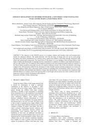
plane, which is orthogonal to (1, 1, 1) , cf. fig. 1. The length
P|ff 1 ,ff 2 ' ff 3'
•» ffi
Fig. 2.1.1: (a) Haigh-Westergaard coordinate system;
(b) Deviatoric plane
b)
of ON is

- 12 -
IONI = £ = OP • e = (a 1 , a 2 , a 3 >
and ON is therefore determined by
^
? I Ij - v*
ON = (1, 1, 1) lj/3
The component NP is given by
NP = OP - ON = ((*]_, o 2 , a 3 ) - (1, 1, 1) 3^/3 = (s 1 , 3 2 , s 3 )
and the length of NP is
INPI = p = (sj 5 + s 2 + s 3 ) 1/2 = /2X
To obtain an interpretation of J, consider the deviatoric plane,
fig. 1 b). The unit vector i, located along the projection of the
a.-axis on the deviatoric plane is easily shown to be determined
by i = (2, -1, -D/V6. The angle 8 is measured from the unit
vector i and we have
p cosB = NP • i
i.e.
cose = vfc (s i' v s 3 ) -å
2
-1
-1
2/3J2~ (2s l' " s 2' " s 3 }
Using s, + s. + s
= 0 we obtain
3s,
cosO = 2VOTJ 2a l ~ a 2 " °3
As a. - a- - o 3 is assumed throughout th*=» text, 0 - 8 - 60
3
holds. Using the identity cos38 = 4 cos 8-3 cos8, the invariant
J in eq. (2) is after some algebra found to be given by
J = cos38 (2.1-3)
The failure criterion eq. (1) can therefore be stated more conveniently
using only invariants as

- 13 -
fd l( J 2 , COS3G) = O (2.1-4)
from which the 60 -symmetry shown in principle in fig. 1 b) appear
J explicitly. The superiority of this formulation or alternatively
f(I , J , C) = 0 compared to eq. (1) appears also clearly
when expressing mathematically the trace of the failure surface
in the deviatoric plane. Generally, only old criteria such as
the Mohr criterion, the Columb criterion and the maximum tensile
stress criterion use the formulation of eq. (1).
The meridians of the failure surface are the curves on the surface
where 8 = constant applies. For experimental reasons, as
the classical pressure cell is most often applied when loading
concrete triaxially, two meridians are of particular importance
namely the compressive meridian where a, = a_ > a., i.e. 9 = 60
holds and the tensile meridian where a, > a_ - a, i.e. 9=0
applies. This terminology relates to the fact that the stress
states a-, = c_ > a ? and a, > a» = a., correspond to a hydrostatic
stress state superposed by a compressive stress in the a_-direction
or superposed by a tensile stress in the a,-direction, respectively.
2.1.2. Evaluation of some failure criteria
Based on the experimental evidence appearing on the following
figures and in accordance with earlier findings of for instance
Newman and Newman (1971) and the writer (1975, 1977), the form
of the failure surface can be summarized as:
1) the meridians are curved, smooth and convex with p increasing
for decreasing £-values;
2) the ratio, p./p , in which indices t and c refer to the tensile
and comp-essive meridians respectively, (cf. fig. 1)
increases from approx. 0.5 for decreasing £- values, but remains
less than unity;
3) the trace of the failure surface in the deviatoric plane is
smooth and convex for compressive stresses;

- 14 -
4) in accordance with 1), the failure surface opens in the negative
direction of the hydrostatic axis.
The tests of Chinn and Zimmerman (1965) alorg the compressive
meridian with a very large mean pressure equal to 26 times the
uniaxial compressive strength support the validity of 4) over a
very large stress range.
Several important failure criteria have been proposed in the past
and some of these have been evaluated by Newman and Newman
(1971), Ottosen (1975, 1977), Wastiels (1979) and by Robutti et
al. (1979). In addition, Newman and Newman (1971), Hannant
(1974) and Hobbs et al. (1977) contain a collection of different
experimental failure data. In this report we concentrate on some
of the several criteria proposed recently and a classical criterion.
The considered criteria are:
- the Reimann-Janda (1965, 1974) criterion originally proposed
by Reimann (1965), but here evaluated by using the coefficients
proposed by Janda (1974). This criterion can be considered
as one of the earliest attempts in modern time to
approximate the failure surface of concrete. Some improvements
of this criterion were later proposed by Schimmelpfennig
(1971).
- the 5-parameter model of Will am and Warnke (1974) that appears
to be the first criterion with a smooth convex trace
in the deviatoric plane for all values of p./p where 1/2 <
p./p £ 1. Its simplified 3-parameter version with straight
meridians has later been adopted by Kotsovos and Newman (1978)
and by Wastiels (1979) using different methods for calibration
of the parameters.
- the criterion of Chen and Chen (1975) may serve as an example
of an octahedral criterion disregarding the influence of the
third invariant, cos38.
- the criterion of Cedolin et al. (1977) corresponds to a failure
surface with a concave trace in the deviatoric plane.

- 15 -
- the criterion proposed by the writer (1977) . This criterion
corresponds to a smooth and convex surface It will be considered
in more details later and it is implemented in the
finite element program.
- the classical Coulomb criterion with tension cut-offs. This
criterion is also implemented in the finite element program
and an evaluation will be postponed until the previously
mentioned criteria have been compared mutally and together
with some representative experimental results.
As mentioned above we will in the first place disregard the Coulomb
criterion with tension cut-offs. The coefficients involved
in the criteria considered are calibrated by some distinct strength
values, for instance, uniaxial compressive strength a (a > 0),
uniaxial tensile strength a. (a > o), etc. In some proposals
such a calibration was already partly carried out leaving only
a few strength values to be inserted by the user, while others
need more strength values. Noting that all coordinate systems
considered here are normalized by a , the applied strength values
are shown in the following table.
Table 2.1-1: Strength values used to calibrate coefficients in
the failure criteria.
V a c
a ,/a
eb' c
£/ø p /a-
' c c c
Vo c
p fc /a c
Reimann-Janda (1965, 1974)
Willam and Warnke (1974)
Chen and Chen (1975)
Cedolin et al. (1977)
Ottosen (1977)
0.08
0.08
0.08
1.15
1.15
-3.20 2.87
-3.20 1.80
a : uniaxial tensile strength (a > o) , a : uniaxial compressive
strength (a > o), a . : biaxial compressive strength (a . > o) .
The additional strength values applied in the Willam and Warnke
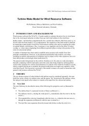
criterion are chosen to fit the experimental data of fig. 2.

- 16 -
Fig. 2 shows the comparison of the considered criteria with some
experimental results (the attention should also be drawn to the
very importc. it international experimental investigation, Gerstle
et al. (1978)). The figure shows the compressive and tensile
meridians. Except for the proposal of Chen and Chen (1975) , a
good agreement is obtained for all criteria. The Chen and Chen
Compressive meridian
P/°C
4
Tensile meridian
p/*c
— Cedolin,etal.(1977)
—Willam and Warnke(197A)
—Reimann-Jonda (1965,197t)
—Ottosen (1977)
Chen and Chen (1975)
O Richartetal.(1928)
• Bolmer (1949)
V Hobbs (1970,1974)
* Kupfer et ol. (1969,1973)
D Ferrara et al. (1976)
Fig. 2.1-2: Comparison of some failure criteria with some
experimental results.

- 17 -
model was used in a strain hardening plasticity theory and to
simplify calculations, it neglects the influence of the angle 0
leading to a large discrepancy for this model when compared with
triaxial experimental results. This will hold for other octahedral
criteria as well, for instance that of Drucker and Prager
(1952). While the failure surface proposed by Willam and Warnke
(1974) intersects the hydrostatic axis for large compressive
loading, in the present case when £/a = -13, the other surfaces
open in the direction of the hydrostatic axis.
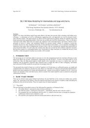
The predicted shape in the deviatoric plane for £/tf = -2 corresponding
to small triaxial compressive loadings, is shown in fig,
3 for the considered criteria. The proposal of Reimann-Janda
EA* = -2
-a 3 /cr c
Cedolin. Crutzen and Dei Poli (1977)
Willam and Warnke (1974)
Reimann - Jando (1965,1974)
Ottosen (1977)
Chen and Chen (1975)
Pig. 2.1-3: Predicted shape in deviatoric plane.

- 18 -
(1965, 1974) and of Cedolin et al. (1977) both involve singular
points, i.e. corners. In addition, the trace of the latter proposal
is concave along the tensile meridian. As will appear
later this concavity has large consequences. The proposal of
Willam and Warnke (1974) and of the writer (1977) both correspond
to smooth convex curves.
Great importance is attached to plane stress states, and fig. 4
a) shows a comparison for all criteria, except that of Cedolin
et al. (1977) with the experimental results of Kupfer et al.
(1969, 1973). All criteria in fig. 4 a) show good agreement with
the experimental data especially those of Willam and Warnke
(1974) and Ottosen (1977) even when tensile stresses occur. Comal
Willam and Warnke (1974)
Reimann-Janda (1965.1974)
Ottosen (1977)
Chen and Chen (1975)
• KupferetaL (1969.1973),

- 19 -
parisons of fig. 2 and 4 a) show that the model of Chen and Chen
(1975) is much more suited for predicting biaxial failures than
tria;:ial ones. For biaxial loading, the proposal of Cedolin et
al. (1977) is compared with the other criteria in fig. 4b). It
appears that the influence of the concavity along the tensile
meridian is ruinous to the obtained curve.
Comparison in general of figs. 3 and 4 reveals that even small
changes in the form of the trace in the deviatoric plane have
considerable effect on the biaxial failure curve. Indeed, the
latter curve is the intersection of the failure surface with a
plane that makes rather small angles to planes which are tangent
to the failure surface in the region of interest. This emphasizes
the need for a very accurate description of the trace in the deviatoric
plane. In general, it may be concluded that fitness of
a failure criterion can be estimated only when comparison.*- with
experimental data are performed in at least three planes of different
type.
2.1.3 The two adopted failure criteria
In the previous section it was shown that the failure criterion
proposed by the writer (1977) is an attractive choice when considering
criteria proposed quite recently. Let us now investigate
this criterion together with the classical Coulomb criterion
with tension cut-offs in more details as both criteria are implemented
in the finite element program.
The criterion proposed by the writer (1977) uses explicitly the
formulation of eq. (4) and suggests that
J ^ I
A ~ + A —^ + B -^i - 1 = 0 (2.1-5)
a c °c c
in which A and B = parameters; and A = a function of cos30,
A = A (cos30) > 0. The value of f(I,, J„, cos36) < 0 corresponds
to stress states inside the failure surface. For A > 0, B > 0 it
is seen that the meridians are curved (nonaffine), smooth and
convex, and. the surface opens in the negative direction of the
hydrostatic axis. From eq. (5)

- 20 -
^2 i r f~2 *! i
~" 2A " A + /X " 4A (B a-M (2' 1 - 6 )
c
L
and it may be shown that when r = l/A(cos36) describes a smooth
convex curve in the polar coordinates (r,0), the trace of the
failure surface in the deviatoric plane, as given by eq. (6) is
also smooth and convex. When approaching the vertex of the failure
surface (corresponding to hydrostatic tension) \/3T-» 0, which
according to eq. (5) leads to
c
J
VJ~ , / I, \ p. A
a - x i 1 - B TJ l - e - ~ -* r for ^ - °
c c e t
(2 - 1 ~ 7)
in which A = A(-l) and A = A(l) correspond to the compressive
and tensile meridian, respectively. As A /A is later determined
to be inside the range 0.54-0.58 (see for comparison, table 3),
eq. (7) indicates a nearly triangular shape of the trace in the
deviatoric plane for small stresses. Furthermore, eq. (6) implies
(P./p ) -* 1 for I 1 -» -», i.e. for very high compressive stresses,
the trace in the deviatoric plane becomes nearly circular. It
was found that the function, A = A(cos30), could be adequately
represented in the form
A = K.^ cos -=• Arccos(K 2 cos39) for cos36 _> 0
A = K^ cosUj - -j Arccos(-K 2 cos30) for cos36 5 0
(2.1-8)
in which K, and K 2 - parameters; K. is a size factor, while K-
is a shape factor (0 - K - 1). This form was originally derived
by a mechanical analogy, as r = l/A(cos39) given by eq. (8)
corresponds to the smooth convex contour lines of a deflected
membrane loaded by a lateral pressure and supported along the ,
edges of an equilateral triangle, cf. appendix A. Thus, r = 1/A
(cos36) represents smooth convex curves with an equilateral triangle
and a circle as limiting cases.

The characteristics of the failure surface given by eqs. (5) and
(8) are: (1) only four parameters used; (2) use of invariants
makes determination of the principal stresses unnecessary; (3)
the surface is smooth and convex with the exception of the vertex;
(4) the meridians are parabolic and opens in the direction of
the negative hydrostatic axis; (5) the trace in the deviatoric
plane changes frcm nearly triangular to circular shape with increasing
hydrostatic pressure; (6) it contains several earlier
proposed criteria as special cases, in particular, the criterion
of Drucker and Prager (1952) for A = 0, A = 'constant, and the
von Mises criterion for A = B = 0 and X = constant.
In evaluating the four parameters A, B, K and K use has been
made of the biaxial tests of Kupfer et al. (1969, 1973) and the
triaxial results of Balmer (1949) and Richart et al. (1928). The
parameters are determined so as to represent the following three
failure states exactly: (1) uniaxial compressive strength o ;
(2) biaxial compressive strength •; , = 1.16 a corresponding to
the tests of Kupfer et al. (1969, 1973) and (3) uniaxial tensile
strength a given by the o /a -ratio (dependence on this ratio
is illustrated in tables 2 and 3). Finally,the method of least
squares has been used to obtain the best fit of the compressive
meridian for f,/a - - 5.0 to the test results of Balmer (1949)
c
and Richart et al. (1928), cf. fig. 5. The compressive meridian
is hereby found to pass through the point (F,/a , p/o ) = (-5.0,
c c
4.0). The foregoing procedure implies values of the parameters
as given in table 2. The values of K, and K- correspond to the
those of A,
t
and A
c
found in table 3.
Table 2.1-2: Parameter values and their dependence on the o./a -
ratio.
1
°t /o c
A
B
K l
« 2 !
' 0.08
0.10
0.12
1.8076
1.2759
0.9218
4.0962
3.1962
2.5969
14.4863
11.7365
9.9110
0.9914
0.9801
0.9647

- 22 -
Table 2.1-3: A.-values and their dependence on the o /a -ratio,
a./a A. A A /A^
t c t c c' t
0.08
: 0.10
14.4725
11.7109
7.7834
6.5315
0.5378
0.5577 .
; 0.12
9.8720
5.6979
0.5772
1
Although the parameters A, B, K 1 and K„ show considerable dependence
on the a t /a c -ratio, the failure stresses, when only compressive
stresses occur, are influenced only to a minor extent.
Using o t /a c = 0.10 as reference, the difference amounts to less
than 2.5%.
Comparison of predictions of the failure criterion with some experimental
results has already been given in figs. 2 and 4. Fig.
5 shows a further comparison with some of the earlier applied
experimental results, but now for a larger loading range. Fig. 6
contains additional experimental results of Chinn and Zimmerman
(1965), Mills and Zimmerman (1970) and the mean of the test results
of Launay et al. (1970, 1971, 1972). Comparisons of the
last two figures indicate considerable scatter of the test results
on the compressive meridian for £,/o < - 5.0, the tendencies
being opposite in the two last figures. Along the tensile meridian
the failure criterion underestimates the results of Launay
et al. (1970, 1971, 1972) and Chinn and Zimmerman (1965) for
C/a c > - 6, in accordance with the higher biaxial compressive
strength determined in these tests (1.8 o and 1.9 a , respectively)
compared with that used to determine the parameters of
the failure criterion. Mills and Zimmerman (1970) determined the
biaxial compressive strength to 1.3 a .
c
If the compressive and tensile meridians are accurately represented,
the trace of the failure surface in the deviatoric plane
is confined to within rather narrow limits provided that the
trace is a smooth, convex curve. This is especially pronounced
when the P t /P c ratio is close to the minimum value 0.5. The a-
bility of the considered failure surface to represent the experimental
biaxial results of Kupfer et al. (1969, 1973) outside the

- 23 -
PM
•—Modified Coulomb
i—Ottosen (1977)
6
5
Compressive
meridian
i.
Tensile
meridian
•C+
-LUniaxial 3 -
»•# compressive i
strength (S T )
A ^2-
Biaxial compressive strength (S 2 )*
Uniaxial tensile strength (S3)
-8 -7 -6 -5 -L -3 -2
-1
-SATe
Fig. 2.1-5: Comparisons of test results by: Balmer (1949) o (Compressive)
; Richart et al. (1928) • (Compressive), +
(Tensile); Kupfer et al. (1969, 1973) a (Tensile)
(Failure stresses S,, S„, S~ and S. determine parameters
in writers failure criterion), c./o = 0.1
used in the criteria.
P
/•Te
r
1
6
I Compressive meridian '
._
5
*
—1_ -
1
^
L
3
2
1
-S/«e
^ig. 2.1-6: Mean values of Launay et al. (1970, 1971, 1972)
(Compressive), (Tensile); Chinn and Zimmerman
(1965) • (Compressive), o (Tensile); Mills and Zimmerman
(1970) • (Compressive) o (Tensile), o./a = 0.1
used in the criteria.

tensile and compressive meridians was shown previously in fig. 4.
However, to facilitate caparison cf Lhe tailure criteria considered
there, not all available experiaental results were giv ^r.
when tensile stresses are present. A sore detailed comparison
with the failure criterion considered now is therefore illustrated
in fig. 7.
a. ;v
i
(12
'-
I
Modified Coulomb
--02
-0.4
j - - -06
•-- Kupfer et al. I 969. 19731
.-0.8
r tt2
Ottosen (1977)
--1.0
•-12
Fig. 2.1-7: Biaxial tests of Kupfer et al. (1969, 1973), - =
58.3 MPa. - = 0.08 a used in both criteria,
t
c
The agreement is considered satisfactory, the largest difference
occurring in compression when • /?-
- 0-5. In this case Kupfer
et al. obtained a, = -1.27 -, as the mean value of tests
2 c
with a
ranging from 18.7 - 58.3 MPa; on the other hand the failure
criterion with the parameters of table 2 gives - 1.35 ' ,
- 1.38 -. and - 1.41 a for a/o = 0.08, 0.10, and 0.12, rec
e t c
spectively. It is interesting to note that the classical biaxial
tests of Wastlund (1937) with a
ranging from 24.5 - 35.0 MPa
give o. = - 1.37 a with almost the same biaxial strength
(1.14 ' ) as the results of Kupfer et al (1.16 n ).
c
c
Suranarizing, the failure criterion given by eqs. (5) and (8) contains
the three stress invariants explicitly and it corresponds
to a smooth convex surface with curved meridians which open in
the negative direction of the hydrostatic axis. The trace in the
deviatoric plane changes from an almost triangular to a more

iL _>
_
circular shape with increasing hydrostatic pressure. The criterion
has been demonstrated to be in good agreement with experimental
results for different types of concrete and covers a
wide range of stress states including those where tensile stresses
iccur. The formulation in terms of one function for all stress
states facilitates its use in structural calculations and it has
been shown that a sufficiently accurate calibration of the parameters
in the criterion is obtained by knowledge of the uniaxial
compressive strength c and the uniaxial strength a alone.
As mentioned previously, the other failure criterion implemented
in the finite element program is the classical Coulomb criterion
with tension cut-offs which consist of a combination of the Coulomb
criterion suggested in 1773 and the maximum tensile stress
criterion often attributed to Rankine, 1876. This dual criterion
was originally proposed by Cowan (1953) but using the terminology
of Paul (1961), it is usually termed the modified Coulomb
criterion. It reads,
ma, - o~. = o
6 C
°1 = °t
(2.1-9)
where, as previously, a, - o - o and tensile stress is considered
positive. The criterion contains three parameters and it
includes a cracking criterion given by the second of the above
two equations. The coefficient m is related to the friction angle
ip by m = (1 + sinip)/(l - sinip) . Different m-values have been proposed
in the past, but here we adopt the value
m = 4 (2.1-10)
corresponding to a friction angle eoual to 37 . This value has
been proposed both by Cowan (1953) and by Johansen (1958, 1959)
and is applied almost exclusively in the Scandinavian countries.
As shown in fig. 8 the modified Coulomb criterion corresponds to
an irregular hexagonal pyramid with straight meridians and with
tension cut-offs. The trace in the deviatoric plane is shown in
fig. 8 together with the other criterion implemented in the fin-

- 26 -
ite program. A comparison with this latter criterion and some
experinental results is shown in figs. 5, 6 and 7.
/-Tension cut-off
5tofc=-2
Modified Coulomb
Ottosen (1977)
Coulomb
Fig. 2.1-8: Appearance of the modified Coulomb criterion.
It appears that for most stress states of practical interest the
modified Coulomb criterion underestimates the failure stresses.
This is quite obvious when considering for instance the case of
plane stress, fig. 7. However, it is important to note that the
modified Coulonu> criterion provides a fair approximation that is
comparable in accuracy to many recently proposed failure criteria
and with the simplicity of the modified Coulomb criterion in
mind it may be considered as quite unique. Note also that just
like the other criterion implemented in the finite element program,
calibration of the modified Coulomb criterion requires
only knowledge of the uniaxial compressive strength a and the
uniaxial tensile strength a for the concrete in question.
In conclusion, the two failure criteria implemented in the finite
element program each provide realistic failure predictions for
general stress states. While the criterion proposed by the writer
(1977) is superior when considering accuracy the modified Coulomb
criterion possesses an attractive simplicity.
2.1.4. Adopted cracking criteria
As the failure criterion proposed by the writer (1977) applies
to all stress states, in terms of one equation, it must be augmented
by a failure mode criterion to determine the possible ex-

- ?7 -
istence of tensile cracks. Following the proposal of the writer
(1979) we assume that the cracking occurs, firstly, if the failure
criterion is violated and secondly, if a, > a./2 holds. Note that
this crack criterion may be applied to any smooth failure surface,
The other failure criterion implemented in the finite element
program - the modified Coulomb criterion - already includes a
cracking criterion determined by a, > a..
1 1 r 1
Concrete 1. o c = 18.7 MPa
ot/Oc,= 0.10usfd in criteria
a y h c
I
0.2-j
-pr—^gracc*"*"—

- 28 -
Figure 9 contains the experimental results of Kupfer et al. (1969,
1973) for biaxial tensile-compressive loading of three different
types of concrete. Both failure stresses and failure modes are
indicated In addition, the figure shows the corresponding failure
curves together with their failure mode criteria using the
two failure criteria implemented in the finite element program.
It appears that the two failure mode criteria and the two failure
criteria are in close agreement with the experimental evidence.
In accordance with earlier conclusions the proposals of
the writer are favourable when considering accuracy. The modified
Coulomb criterion , on the other hand, possesses an attractive
simplicity.
For both failure mode criteria it is assumed that the orientation
of the crack plane is normal to the principal direction
of o.. This assumption is also in good agreement with the aforementioned
tests.
2.2. Stress-strain relations
Having discussed the strength of concrete in some detail, the
stress-strain behaviour will now be dealt with. Ideally, a constitutive
model for concrete should reflect the strain hardening
before failure, the failure itself as well as the strain softening
in the post-failure region. The post-failure behaviour has
received considerable attention in the last years especially,
where it has become evident that the calculated load capacity of
a structure may be strongly influenced by the particular postfailure
behaviour employed for the concrete; for example ideal
plasticity with its infinite ductility might be an over-simplified
model. This is just to say that redistribution o i stresses
in a structure must be dealt with in a proper way. These aspects
will be considered in some detail in section 5. Moreover, the
constitutive model should ideally be simple and flexible, i.e.
different assumptions can easily be incorporated. The numerical
performance of the model in a computer program should also be
considered. Moreover, it should be applicable to all stress
states and both loading and unloading should ideally be dealt

- 29 -
with in a correct way. Eventually, and as a very important feature,
the model should be easy to calibrate to a particular type
of concrete. For instance it is very advantageous if all parameters
are calibrated by means of uniaxial data alone.
A model reflecting most of the above-mentioned features will be
described in the following, but prior to this attention will be
turned towards the large number of proposals for predicting the
nonlinear behaviour of concrete that have appeared in the past.
Plasticity models have been proposed; however because of their
simplicity the bulk of the models are nonlinear elastic ones. A
review of some models is given as follows:
Plasticity models based on linear elastic-ideal plastic behaviour
using the failure surface as yield surface have been proposed
by e.g. Zienkiewicz et al. (1969), Mroz (1972), Argyris
et al. (1974) and Willam and Warnke (1974). A somewhat different
approach still accepting linear elastic behaviour up to failure
was put forward by Argyris et al. (1976) using the modified Coulomb
criterion as failure criterion. Instead of a flow rule this
model uses different stress transfer strategies when stresses
exceed the failure state. A very essential feature is that different
post-failure behaviours can be reflected in the model. To
consider the important nonlinearities before failure, models
using the theory of hardening plasticity have been proposed by
e.g. Green and Swanson (1973), Ueda et al. (1974) and Chen and
Chen (1975), all of whom neglect the important effect of the
third stress invariant, while Hermann (1978) includes the effect.
However, as these plasticity models all make use of Drucker's
stability criterion (1951) they are not able to consider the
strain softening effects occurring after failure. Coon and Evans
(1972) applied a hypoelastic model of grade one, but this model
also operates with two stress invariants only, and strains are
inferred as infinite at maximum stress.
Incremental nonlinear elastic models based on the Hookean anisotropic
formulation have been proposed for plane stress by Liu
et al. (1972) and Link et al. (1974, 1975). The model of Darwin
and Pecknold (1977) applicable for plane stresses can even be

- 30 -
used for cyclic loading in the post-failure region. In contrast
to these proposals, similar models that now assume the incremental
isotropic formulation neglect the stress-induced anisotropy,
and softening and dilatation cannot be dealt with. This is because
tangential values of Young's modulus and Poisson's ratio can
never become negative or larger than 0.5, respectively. However,
a tangential formulation facilitates the numerical performance
regarding convergence in a computer cjde. A model based on this
incremental and isotropic concept and applicable for general
plane stresses was introduced by Romstad et al. (1974) using a
multilinear approach. In the models proposed by Zienkiewicz et
al. (1974) and Phillips et al. (1976) the tangential shear irodulus
variates as a function of the octahedral shear stress
alone. In principle, a similar approach applicable for compressive
stresses and valid until dilatation occurs was later applied
by Riccioni et al. (1977), but in this model the influence of
all the stress invariants on both the tangential bulk modulus
and the tangential shear modulus was considered. Recently, Bathe
and Ramaswamy (1979) proposed a model considering all stress invariants
also and applicable for general stress states while the
Poisson ratio was assumed to be constant.
Several nonlinear elastic models of the Hookean isotropic form
using the secant values of the material parameters have also
been put forward. An early proposal of Saugy (1969) considered
the bulk modulus as a constant and the shear modulus as a function
of the octahedral shear stress alone. For plane compressive
stresses Kupfer (1973) and Kupfer and Gerstle (1973) assumed both
these moduli to be functions of the octahedral shear stress. PTlamiswamy
and Shah (1974) and Cedolin et al. (1977) proposed nudels
applicable to triaxial compressive stress states also. Hovever
only the influence of the first two stress invariants on
the bulk and shear moduli are considered and the validity of the
models is limited to stress states not too close to failure. Also
the recent approach by Kotsovos and Newman
(1973) neglects the
influence of the third invariant. Schimmelpfennig (1975, 1976)
made use of a model where the shear modulus changes. All stress
invariants are considered but only compressive stress states can
be dealt with, and dilatation is excluded.

- 31 -
All the nonlinear elastic models mentioned previously, except
the proposals of Romstad et al. (1974), Darwin and Pecknold
(1977), Bathe and Ramaswamy (1979) and to some extent, that of
Riccioni et al. (1977), have to be argumented by a failure criterion
that is formulated completely independently of the stressstrain
relations presented. This results in a nonsmooth transition
from the prefailure behaviour to the failure state. In addition,
all these models, except again, the model of Romstad et al.
(1974), Darwin and Pecknold (1977), Bathe and Ramaswamy (1979)
and to some extent, the model of Cedolin et al. (1977), are valid
only for a particular type of concrete. As a result, the models
can only be calibrated to other types of concrete if, in addition
to uniaxial results, biaxial or triaxial test results are also
available for the concrete in question.
Recently, Ba^ant and Bhat (1976) extended to endochronic theory
to include concrete behaviour. Very important characteristics such
as dilatation, softening and realistic failure stresses are simulated
and the model can be applied to general stress states even
for cyclic loading. In a later version of the model, Bazant and
Shieh (1978), even the nonlinear response to compressive hydrostatic
loading was reflected. However, Sandler (1978) has questioned
the uniqueness and stability of the endochronic equations
and the modelling only through the value of the actual concrete's
uniaxial compressive strength is another important aspect. This
seems to be a rather crude approximation even for uniaxial compressive
loading, as different failure strains and initial stiffnesses
can be obtained for concrete possessing the same uniaxial
compressive strength.
The following model proposed by the writer (1979) for the description
of the nonlinear stress-strain relations of concrete
is based on nonlinear elasticity, where the secant values of
Young's modulus and Poisson's ratio are changed appropriately.
Path-dependent behaviour is naturally beyond the possibilities of
the model and the same holds also for a realistic response to
unloading when nonlinear elasicity is used. However, from the way
in which the model is implemented in the program, cf. section
4.6, its unloading characteristics is greatly improved compared

- 32 -
to that of nonlinear elasticity and the model indeed corresponds
to the bei aviour of a fracturing solid, Dougill (1976). Moreover,
the described model is able to represent in a simple way most
of the characteristics of concrete behaviour, even for general
stress states. These features include: (1) the effect of all three
stress invariants; (2) consideration of dilatation; (3) the obtaining
of completely smooth stress-strain curves; (4) prediction
of realistic failure stresses; (5) simulation of different
post-fajlure behaviours and (6) the model applies to all stress
states including those where tensile stresses occur. In addition,
the model is simple to use, and calibration to a particular type
of concrete requires only experimental data obtained by standard
uniaxial tests. The construction of the model can conveniently
be divided into four steps: (1) failure and cracking criteria;
(2) nonlinearity index; (3) change of the secant value of Young's
modulus and (4) change of the secant value of Poisson's ratio.
The failure and cracking criteria utilized in this section are
the ones proposed by the writer and dealt with in sections 2.1.3
and 2.1.4. In the finite element program the modified Coulomb
criterion described previously is also used together with the
following stresr-strain model and it should be emphasized that
any failure criterion can be employed in connection with the described
constitutive model, and no change as such is necessary
because the criterion in question i s involved only througn the
determination of the nonlinearity index, as defined.
2.2.1. Nonlinearity index
Let us now define a convenient ir ;asure for the given loading in
relation to the failure surface. First of all, we have to determine
to which failure state the actual stress state should relate.
Although there is an infinite number of possibilities,
four essentially different types can be identified. To achieve
a simple illustration, we will at present adopt as failure criterion
the Mohr criterion shown in fig. 1 a), which also shows
the actual stress state given by a, and o~. Failure can be obtained
by increasing the a,-value as shown by circle I, or alternatively
by fixing the (o, + o,)/2-value as shown by circle II.
However, tensile stresses may then be involved in the failure

- 33 -
state as shown in fig. 1 a) and an evaluation of, e.g., a uniaxial
compressive stress state, would depend on the tensile
^-failure curve
»=s
X
in/ IY/
n/v^S
i : i l \
— a
" ^

- 34 -
of being proportional to the stress for uniaxial compressive
loading, i.e., it can be considered as an effective stress. Note
that the nonlinearity index depends on all three stress invariants
if the failure criterion does also. The |3-values will later
be used as a kind of measure for the actual nonlinearity; fig. 2,
where the failure criterion proposed by the writer (1977) is
applied and where contour lines for constant B-values are shown,
demonstrates its convenience for this purpose. Fig. 2 a) shows
meridian planes containing the compressive and tensile meridian.
Points corresponding to the uniaxial compressive strength, S.,
and the biaxial compressive strength, S 2 , are shown on these meridians,
and failure states involve tensile stresses to the right
of these points. Fig. 2 b) shows curves in a deviatoric plane.
Note in fig. 2 a) that in contrast to the failure surface, sura)
b)
Fig. 2.2-2: Contour lines of constant B-values. (a) Meridian
planes, S, = uniaxial compressive strength, S~ = biaxial
compressive strength, S 3 = uniaxial tensile
strength; (b) Deviatoric plane. Failure criterion
proposed by the writer (1977) is applied.
faces on which the nonlinearity index is constant are closed in
the direction of the negative hydrostatic axis. For small £-
values, these surfaces resemble the one that defines the onset
of the stable fracture propagation, i.e. the discontinuity limit
(see, for comparison, Newman and Newman (1973) and Kotsovos and

- 35 -
Newman (1977)) -
When tensile stress occur, a modification of the definition cf
the nonlinearity index is required as concrete behaviour becomes
less nonlinear, the more the stress state involves tensile stresses.
For this purpose we transform the actual stress state
(a., a«, a.,), where at least o^ is a tensile stress, by superposing
the hydrostatic pressure, ~ 0 -i» obtaining the new stress
state (a*, a', o^) = (0, a_ - c^, a 3 - a ± ),
i.e. a biaxial compressive
stress state. The index B is then defined as
6 = -4- (2.2-2)
°3f
In which al f is the failure value of a' provided that a'
and a^
are unchanged, i.e. the stress state (a 1 , a', o' f ) is to satisfy
the failure criterion. This procedure has the required effect,
as shown in fig. 2 a), of reducing the 3-values appropriately
when tensile stresses occur and 3 < 1 will always apply. Point
S 3 on fig. 2 a) corresponds to the uniaxial tensile strength,
and B = 0 holds for hydrostatic tension. Contour surfaces for
constant (3-values are smooth, except for points where tensile
stresses have just become involved.
2.2.2. Change of the secant value of Youngs's modulus
To obtain expressions for the secant value of Young's modulus
under general triaxial loading, we begin with the case of uniaxial
compressive loading. Here we approximate the stress-strain
curve as proposed by Sargin (1971)
-A f- + (D-l) ( | - ) 2
" T = S —7 T-2 < 2 - 2 " 3 >
°c l-(A-2) £- + D (—) Z
e e
c c
Tensile stress and elongation are considered positive, and e
determines the strain at failure, i.e., c = - e when a = - a .
The parameter A is defined by A = E./E , in which E = a /e .
The Young's moduli E. and E are the initial modulus and the sei
c
cant modulus at failure, respectively? D = a parameter mainly

- 36 -
affecting the descending curve in the post-failure region. Eq.
(3) is a four-parameter expression determined by the parameters
a , e , E., and D, and it infers that the initial slope is E.,
and that there is a zero slope at failure, where (a,e) = (- c ,
-e ) satisfies the equation. The parameter D determines the postfailure
behaviour, and even though there are some indications of
this behaviour, e.g. Karsan and Jirsa U969),the precise form of
this part of the curve is unknown and is in fact, not obtained
by a standard uniaxial compressive test. Therefore, the actual
value of D is simply chosen so that a convenient post-failure
curve results. However, there are certain limitations to D, if
eq. (3) is to reflect: (1) an increasing function without inflexion
points before failure; (2) a decreasing function with at
most one inflexion point after failure; (3) a residual strength
equal to zero after sufficiently large strain. To achieve these
features A > 4/3 must hold, and the parameter D is subject to
the following restrictions
(1-35A) 2 < D _< l+A(A-2) when A < 2;
0 _< D 4/3 is in practice not a restriction, and, in
fact, eq. (3) provides a very flexible procedure to simulate the
uniaxial stress-strain curve. For instance, the proposal of Saenz
(1964) follows when D = 1, the Hognestad parabola (1951) follows
when A = 2 and D = 0, and the suggestion of Desayi and Krishnan
(1964) follows when A = 2 and D = 1. In addition, different postfailure
behaviours can be simulated by means of the parameter D
and this affects only the behaviour before failure insignificantly.
This is shown in fig. 3, where A = 2 is assumed and where
the limits of n are given by zero and unity.
Using simple algebra, eq. (3) can be solved to obtain the actual
secant value E
s
of Young's modulus. The expression for E
s
con-
tains the actual stress in terms of the ratio - 0/0 . For unic
axial compressive loading £ = - a/a
for E
holds, and the expression
can therefore be generalized to triaxial compressive load-

°
b
-1.2
-1.0
-0.8
0.6
-0.4
-0.2
!
/
//
//
//
il
I
'
I r I
^Desayi & Krisbnon
HognestodX A=2. D = 1
A=2, D=O;
nn
i i . \ i I
0.0 -0.5 -1.0 -1.5 -2.0 -2.5 -3.0 -3.5
Fig. 2.2-3: Control of post-failure behaviour by means of parameter
D in eq. (3) .
ing, if we replace the ratio - o/a
by £. We then obtain
E
2.„2,
s = ^E i -B(^E i -E f )+\/[55E

- 33 -
E f " I"« 4(A C -1) x
{2 - 2 " 5)
in which x represents the dependence on the actual loading and
X/^m Thc
is given by x =

- 39 -
E =
8E WXT E_ E„
MN A M
E»F„ + B«E MXT (E„ - Ej
A M f MN V M
(2.2-6)
in which E
, depending on B, is the secant value along the original
post-failure curve MN obtained by means of eq. (4), using
the negative sign. Likewise, the constants E, and E,„ are secant
A M
values at failure also determined by eq. (4) using the positive
and negative sign, respectively, and the nonlinearity index value
at failure, i.e. B = B f - The preceding moduli are shown in fig.
4. Eq. (6) implies a gradual change of the post-failure behaviour,
both when the stress state is changed towards purely compressive
states, or towards stress states where cracking occurs.
1.0
Pi
0.6
P
0.2
" A/
— Æ ^
-/E 4
//
.•••.
• — •
'•.
1 'V
M
-*.
/ :
VE M '••
/
• •
••.
'"-•,
> •
"...N
—
-
-
Fig. 2.2-4: Post-failure behaviour for intermediate stress states
that do not result in cracking or compressive crushing
of concrete.
2.2.3. Change of the secant value of Poisson's ratio
Let us now turn to the determination of the secant v.lue u of
s
Poisson's ratio. Both for uniaxial and triaxial compressive loading
we note that the volumetric behaviour is a compaction followed
by a dilatation. The expression of M
for uniaxial compressive
loading is therefore generalized to triaxial compressive
loading by use of the nonlinearity index B. Hereby we obtain
u = u. when B < B_
S I —a
u s -
u f - (u f - v A - (i^) : (2.2-7)
when B > B
" a,
in which u ± = the initial Poisson ratio; and u f » the secant
value of Poisson's ratio at failure. Eq. (7) is shown in fig. 5

- 40 -
1.0
i i 1 r
0.6
0.2
J I I L
0.2 0.4
v s
Fig. 2.2-5: Variation of secant value of Poisson's ratio.
The second of these equations, which represents one-quarter of
an ellipse, is valid only until failure. Very little is known of
the increase of u in the post-failure region, but it is an experimental
fact that dilatation continues here. Now, for a given
change of the secant value E , there corresponds a secant value
u*, so that the corresponding secant bulk modulus is unchanged.
In this report, we decrease the E value by steps of 5% in the
post-failure region, and to ensure dilatation in this region
also we then simply put u = 1.005 u* in each step, although
other values may also be convenient. A similar approach is usea
for the intermediate stress states where tensile stresses are
present but no cracking occurs. In the model, u < 0.5 must always
hold, but this limit is achieved only far inside the postfailure
region. In eq. (7), a fair approximation is obtained
when the following paraireter values are applied for all types of
loading and concrete
0 a = C.8; u f = 0.36 (2.2-8)
As before, the 8 value to be applied in eq. (7) is determined
by eq. (1) when only compressive stresses occur, and by eq. (2)
when tensile stresses are present.
In summary, the constitutive model is based on nonlinear elasticity,
where the secant values of Young's modulus E , and
Poisson's ratio u , are changed appropriately. We select a failure
criterion, and on this basis calculate the nonlinearity index

defined by eq. (1), when compressive stresses alone occur, and
by eq. (2) when tensile stresses are present. Here we apply the
failure criterion proposed by the writer (1977), but any criterion
can be used, and the choice influences only the 3 value.
The secant value E is given by eq. (4) coupled with eq. (5)
when compressive stresses occur alone, and coupled with E f = E
when tensile stresses are present. The secant value is given
by eqs. (7) and (8). The model is calibrated by six parameters:
the two initial elastic parameters, E. and u., the two strength
parameters, a
and o , the ductility parameter e , and finally
the post-failure parameter D. While the D value is chosen, following
earlier remarks, so that a convenient post-failure behaviour
is obtained the other parameters are found from standard
uniaxial tests. Let us now illustrate the abilities of the model
by comparing its predictions with experimental results arrived
at for different types of concrete under various loadings.
2.2.4. Experimental verification
The biaxial results of Kupfer (1973) including tensile stresses,
are considered first. Fig. 6 shows the comparison between the
predictions of the model and the experimental results. The concrete
has a rather low strength. The following parameters were applied
in the model: E. = 2.89 • 10 4 MPa, u. = 0.19, a = 18.7 MPa,
i i c
o /a = 0.1, e =1.87 o/oo, and D = 0. Fig. 6 a) shows the cases
of uniaxial and biaxial compressive loading, and fig. 6 b) shows
the volumetric behaviour connected with these loadings. Fig. 6 b)
(a)
i l i i i
-1.2
El
-1.0
,-0.8
'-0.6
e r- E 2/
Uniaxial and biaxial
>A
1
_ 0 , ' (o- 2 /

Uniaxial and biaxial (

- 43 -
demonstrates that the model is able to simulate the dilatation
that is characteristic for concrete loaded in compression. The
behaviour of concrete becomes less nonlinear, the more the stress
state involves tensile stresses; this fact is shown in fig. 6 c)
for a biaxial tensile-compressive loading and in fig. 6 d) for
uniaxial and biaxial tensile loadings. The loadings in fig. 6 c)
and 6 d) result in cracking, i.e. a completely brittle failure.
Stress-strain curves for triaxial compressive loading obtained
by means of the classical pressure chamber method and resulting
in failure along the compressive meridian (c, = c~ > ^3) are
shown in both figs. 7 and 8. To indicate their appearance, the
predicted stress-strain curves on these figures are also indicated
at the beginning of the post-failure region, even though
no experimental data were given there.
150
125 -

- 44 -
-300

45 -
2.3 Creep
Even though the finite element program and therefore also the
present report concentrate on short-term loading of structures
until failure occurs, nonlinearities due to time effects, i.e.,
creep strains, will be touched upon as the program enables one to
deal with creep effects caused by simple load histories. This is
done using the simple "effective E-modulus" concept described
below.
For concrete structures subjected to normal loads it is usually
assumed that concrete behaves like a linear viscoelastic material.
For instance, the resulting proportionality between
creep strains and stresses is generally considered as valid for
uniaxial compressive loading provided the sustained stress is
below half the short-term strength, cf. for instance Browne and
Blundell (1972) . Therefore for a constant uniaxial stress o we
have
e C = £ SP a (2.3-1)
c
sp
where e is the creep btrain and c is termed in the specific
creep function, i.e., the creep strain for unit stress. The specific
creep function depends in general on time t and temperature
T i.e. e sp = e p (t,T). If concrete is considered to be a
homogeneous and isotropic material then two material parameters
define the material also when creep strains are involved, cf.
for instance Nielsen et al. (1977). These two parameters may be
considered as the creep Young's modulus and the creep Poisson's
ratio that now depend on time and temperature. Experiments show,
cf. for instance Browne and Blundell (1972) and Hannant (1969)
that Poisson's ratio during creep can be assumed to be equal to
Poisson's ratio during short-term loading. This leaves Young's
modulus during creep to be determined. For this purpose we consider
a constant uniaxial stress state. The total strain e cone
c
sists of the elastic strain r. and the creep strain E i.e.
_
E = E
e
J.
+ E
c

- 46 -
Using Hooke's law and eq. (1) we obtain
e = | • ; SP a (2-3-2)
where E is Young's modulus during short-term loading. From eq.
(2) we derive
where
eff
Hannant (1969) has shown that creep even under sustained triaxial
loading can be estimated with close accuracy from uniaxial
creep data using the above concept.
The modulus E , f is termed the "effective E-modulus" as it appears
that a creep calculation using the finite element program
can be performed as a usual elastic calculation where the modulus
E is simply replaced by E ff according to eq. (3). It
should be noted that this "effective E-modulus" concept assumes
in principle that stresses are constant throughout the loading
time, but even for constant loading, stress redistributions due
to creep will in general occur in the structure thereby violating
in principle the basis of the approach. Nevertheless,
these latter stress changes are often quite small but it emphasizes
that the "effective" E-modulus" concept must be utilized
with caution. However the appeal of the method is its extreme
simplicity.
Presently, the specific creep function available in the prograin
is that proposed by Cederberg and David (1969) i.e.
e sp = 10" 6 (0.4 + 0.086 • T) In (1 + t) [MPa]" 1 (2.3-4)
where T is the temperature in °C and t the loading time in days.
Moreover, the short-term modulus E in eq. (3) is assumed to depend
on the temperature according to

- 47 -
E(T) = E (1-04 - 0.002 • T) (2.3-5)
o
where E is the modulus at 20 C. Eq. (5) was also proposed by
Cederberg and David (1969).
With these few remarks no more attention will be drawn toward
time-dependent behaviour of concrete as the primary concern of
the present study is that of concrete structures loaded in the
short-term until failure.
2.4. Suitunary
The present section 2 has primarily dealt with failure and nonlinear
behaviour of concrete when loaded in the short-term by
general stress states. Different failure criteria and their a-
greement with experimental result have been discussed and it has
been shown that the two failure criteria dealt with in section
2.1.3 and the failure mode criteria dealt with in section 2.1.4
provide a realistic approach to actual behaviour. In particular,
it has been shown that the criterion of the writer (1977) is
superior when considering accuracy, whereas the modified Coulomb
criterion possesses an attractive simplicity. In section 2.2 a
model for the stress-strain behaviour of concrete was outlined.
This model, proposed by the writer (1979) and implemented in
the finite element program, is based on nonlinear elasticity,
where the secant values of Young's modulus and Poisson's ratio
are changed appropriately.
The model simulates the nonlinear behaviour before failure, as the
failure itself and as the post-failure behaviour. Smooth stressstrain
curves are obtained, and different post-failure behaviours
can easily be produced by changing one parameter, D, alone, while
changing only the behaviour before failure insignificantly. In
addition, the model reflects the dilatation that occurs when
concrete is loaded in compression and the influence of all three

- 48 -
stress invariant is considered.
Through use of the nonlinearity index, 0, relating the actual
stress state to the failure surface, the model can be applied
without change in connection with any failure criterion, and
choice of an accurate failure criterion by itself assures predictions
of realistic stress-strain curves. The constitutive
model applies to all stress states, including those where tensile
stresses are present. The model is determined by only six
parameters that depend on the actual concrete. These are the
initial elastic parameters, E. and u., the strength parameters
a and o , the ducility parameter, e , and the post-failure
parameter, D. The calibration of the model is easily performed,
as the D value is chosen to correspond with the anticipated
post-failure behaviour. The other parameters are obtained by a
standard uniaxial compressive, and a standard uniaxial tensile
test. The flexibility of the model and its unified formulation
makes it suitable for use in computer codes when investigating
the sensivity of structures to certain specific parameters, e.g.,
the influence of different failure criteria, different post-failure
behaviors, etc.; this will in fact be demonstrated in section
5. In the present section, however, it has been shown that
the model predictions are in good agreement with experimental
results over a wide range of stress states also including tensile
stresses, and obtained by using very different types of
concrete.
3. CONSTITUTIVE EQUATIONS FOR REINFORCEMENT AND PRESTRESSING
Plastic deformations of reinforcement embedded in the concrete
and of unembedded reinforcement, i.e., springs can be dealt with
in the finite element program. In practice, unembedded reinforcement
often corresponds to ungrouted prestressed tendons, but prestressing
of the springs is not mandatory. The following uniaxial
stress-strain relations aie assumed to apply for usual reinforce-

- 49 -
ment and for unembedded reinforcement:
a
•i
ii
a
*- e ^ _ E
a) usual reinforcement b) unembedded reinforcement
Fig. 3-1: Uniaxial stress-strain curves for usual reinforcement
and for unembedded reinforcement.
I.e. a trilinear stress-strain curve applies to usual reinforcement
while a quadrilinear stress-strain curve applies to unembedded
reinforcement. The slope of the lines is arbitrary except
that it is non-negative. In the present section emphasis is given
not to the constitutive modelling as such, as it is quite trivial,
but rather to a formulation that is computationally convenient
in the finite element program.
As outlined in section 4.3 usual reinforcement may consist of
bars or of membranes while unembedded reinforcement, i.e., springs,
obviously are treated as uniaxial loading. In accordance with
the formulation of the constitutive equations for concrete in
terms of secant values of Young's modulus and Poisson's ratio,
the constitutive equations for usual reinforcement are based on
a total formulation instead of the generally more accurate incremental
formulation. For usual bars carrying stresses in one
direction only the two formulations coincide when loading alone
is considered, but for membrane reinforcement differences exist.
The incorrect response to unloading inherent in the total formulation
employed is considered to be of minor importance as only
structures subject to increasing external loading are dealt with.
For unembedded reinforcement, i.e., springs, a different approach
is followed that considers both loading and unloading in a correct
way. This numerical approach is outlined in section 4.4 and
no more attention will be given here to unembedded reinforcement

- 50 -
as the constitutive behaviour is fully described by fig. 3-1 b).
In the present section we proceed with the total formulation of
the plasticity theory as applied to membrane reinforcement.
The von Mises yield criterion is employed and considering in the
first place the incremental formulation of isotropic hardening
this means that the loading surfaces are given by
f - (I s i: Hif " a e leP »
(3 ' 1)
where s.. as usual is the deviatoric stress tensor and a is the
in
e
equivalent stress. In accordance with the assumption of isotropic
hardening a depends on the equivalent plastic strain e . The
increment of equivalent plastic strain e is defined by
where z. . denotes the plastic strain tensor. For uniaxial loading,
eq. (1) infers that f = a,, = a . Assuming the usual normality
rule following for instance from Drucker's postulates (1951) we
have
de?. = dX |£
where dX is a positive function. Use of eq. (1) yields
de ?j • dA rir 1 < 3 - 3 '
e
From the latter equation follows plastic incompressibility which
in turn implies that for uniaxial loading eq. (2) results in
de p = dz\ v
If eq. (3) is multiplied with itself we obtain
ax - (2 de?, deP j ) %
i.e.
dX » d£ p

- 51 -
By use of eq. (3) we have then derived the final incremental
equations
deP . d£P llil (3_ €)
J
e
where de is given by eq. (2) and a by eq. (1).
If increasing proportional loading is considered it follows
that
J
where the ratio s. ./a
lj e
that
e
is constant. From this equations follows
^
£P= U £?. ,*.)* (3-6)
\3 13 13/
Eqs. (5) and (6) hold exactly for increasing proportional loading.
It is now assumed that they also apply to nonproportional
loadings. However, while in the finite element program the reinforcement
stresses are not directly determined, the total reinforcement
strains are known as these are assumed to be identical
to the concrete strains. It is therefore advantageous to derive explicitly
the relation between reinforcement stresses and total
strains. Noting that total strains e.. are composed of elastic
strains e . . and plastic strains e?. i.e.
e. . = e e . + e?. (3-7)
13 13 13
and working only with principal stresses and strains which is
allowable here inasmuch as the corresponding principal directions
always are assumed to coincide, we therefore write
1 e P
e 1 = - (o x - u(o 2 + o 3 )) + 35- (2 0;L - o 2 - o 3 )
e
e 2 = | (o 2 - u«^ + o 3 )) + fj- (2G 2 - o 1 - o 3 >
e
1 £ P
c 3 = s (o 3 - .j( 0l + o 2 )) + jo - (2o 3 - °1 " a 2>
e

- 52 -
where Hooke's law and eq. (5) are applied. Solving this equation
system so that stresses are given in terms of strains and putting
c^ = 0 in accordance with the assumption that plane stresexists
in the membrane reinforcement we obtain
£ 3 = " I=S U l + £ 2 ) (3-8)
and
where
r f
a, R S e.
1
L
_ J.
=
a_ « 2 -S 2 S

- 53 -
As the total strains are composed of elastic and plastic strains
it follows from eq. (11) that
1
E
r
1
-u
"I
-u
1
r
a oi
a 02
(3-13)
r
Equation (11) and (12) form the basis for the initial stress
method employed in the program for consideration to nonlinearities
in membrane reinforcement, cf. section 4.3.2.
However, some furthe.- derivations are necessary as the finite
element program directly determines only the total strains and
also because the only quantities that are stored from the previous
loading stage are the initial stresses. Parameters R and
S present in eq. (12) and defined by eq. (10), however, require
knowledge of the equivalent stress a and the equivalent plastic
strain e both corresponding to the actual total strains. Using
the plastic incompressibility, eq. (6) can be written
£ P =
VT V/E?2 + e5 ? + e? e? (3-14)
Through eqs. (13) and (14) the equivalent plastic strain e p
tuereby also the equivalent stress a
can be determined, both
corresponding to the previous loading stage. Obviously, an iteration
sequence is necessary to determine the present values of
e p and a and different iteration schemes can be employed for
e
this purpose. Here we make use of the proposal of Mendelson
(1968) which has the advantage of quick convergence and applicability
even in the case of ideal plasticity. In essence this proposal
given below enables one to compute plastic strains from
total strains without recourse to stresses.
Letting e ±j = c ±j - §
and
.., e kk and ej., = z e ±. - ± 6. . ej fc denote
the deviatoric total strain and the deviatoric elastic strain,
respectively, and noting that the plastic strain tensor e?. is
purely deviatoric, eq. (7) yields

e.. = e e . + eP (3-15)
ID i] i]
From Hooke's law follows
e
e ij
= fil
2 G
where G is the shear modulus. Inserting this equation in eq. (15)
and eliminating s.. by means of eq. (5) gives
e.. = (-^- + l) e?. (3-16,
ID v 3Ge p ; ID
Multiplication of eq. (16) with itself yields
FP = e _ e(e y ) (3-17)
e e et 3G
where eq. (6) has been used and where the equivalent total
strain e . is defined by
e et
= (I „ e .Y«
V3
.. e..)
i] ID/
which using the definition of deviatoric total strain can be
written
e et = -2 ^Ul
~ £ 2 )2 + (£ 1 " e 3 )2 + (c 2 " e 3 )
Moreover, as the stress-plastic strain curve obtained from uniaxial
loading and derived from fig. 3-1 a) determines a as a
p
unique function of e , equation (17) is the expression sought,
as it determines the equivalent plastic strain e p as a function
of e . determined by the total strains. The iteration sequence
is then as follows:
From the present values of the total strains e, and e„ and from
the values of o and e p from the previous loading stage a e,-
value is determined through eq. (8). The equivalent total strain
e . is then evaluated by means of eq. (10) . Knowing e . and a ,
eq. (17) determines a new value of e p and thereby also a new
value of a . This iteration loop is continued until values for
e p and o that are in suffficiently close agreement with the pre-

- 55 -
sent values of total strains e, and e_ are obtained. The initial
stresses in question can then be determined through eq. (12).
For uniaxial reinforcement bars the approach is much simpler.
As perfect bond is assumed, the axial strain e is directly determined
in the finite element program. Through the uniaxial
stress-strain curve of fig. 3-1 a) the corresponding stress is
determined, i.e.,
a = a (e)
This constitutive equation is equivalent to
a = Ee + a_
where the initial stress is given by
o Q = a(e) - Ee (3-19)
No iteration sequence is involved here.
Summarizing, the constitutive equations for usual embedded reinforcement
corresponds to nonlinear elasticity. The numerical
considerations of plastic deformation are applied using the i-
nitiai stress method outlined in section 4.3.2. For a given
loading stage, the finite element program determines the total
strains in the reinforcement plane. For membrane reinforcement
the corresponding initial stresses are given by eq. (12) while
the initial stress for uniaxial reinforcement bars is given by
eq. (19).
4. FINITE ELEMENT MODELLING
In this section the finite element formulation of the AXIPLANEprogram
described by the writer (1980) is given.
This pro-

- 56 -
gram is applicable for axisymmetric, plane stress and plane
strain structures. Triangular elements are utilized for simulation
of concrete, while one- and two- dlnensional elements simulate
arbitrarily located reinforcement bars and membranes- Linear
displacement functions are used in all elements resulting in
perfect bond between concrete and steel. Figure 1 shows the
available axisymmetric elements while figs. 2 and 3 show the
plane stress and plane strain elements, respectively. These
I Concrete element
* Tangential bars
^ =
— R
l Bars in RZ-plane
Membrane
i
— R
— R
Fig. 4-1: Axisymmetric elements,
I Concrete element
| Bars in XY-plane
-X • — X
Fig. 4-2: Plane stress elements.
figures also illustrate bow the discrete reinforcement bars are
smeared out to equivalent "shells" possessing identical volumina
and stiffness characteristics as the bars. It is apparent that

- O i —
Y
I Concrete element
Y
I Bars in XY-piane
L.
~x
-X
Membrane parallel
to the Z - axis
/
Z
Fig. 4.3: Plane strain elements.
from a finite element point of view, the modelling is very simple.
It also follows that the program is most suited for analysis of
massive structures while slender structures acting primarily in
bending represent problems that are unfitted for use of the program.
In section 4.1 following, the fundamental equations in the finite
element displacement method will be derived. Then, sections
4.2, 4.3 and 4.4 will treat the axisymmetric elements in detail.
The formulation of the plane elements follow very much the same
lines and they will therefore be treated only schematically in
section 4.5. Finally, the computational schemes employed in the
program will be considered in section 4.6.
4.1. Fundamental equations of the finite element method
This section briefly outlines the fundamental equations of the
finite element displacement method. The Galerkin method is util-

- p o ­
ized in this formulation for the following reasons: (1) it operates
directly with the differential equations in question and
no corresponding functional or potential function is needed opposed
to the Rayleigh-Ritz method; and (2) it demonstrates clearly
which equations are satisfied exactly and which only approximately.
The present section takes some advantage of the work of
Zienkiewicz (1977) pp. 42-92. Cartesian coordinates are assumed
and tensor notation is used for lower indices with Latin letters
ranging from 1 and 3 and Greek letters ranging from 1 to n or
from 1 to n .
Five basic equations define the response when a structure is
loaded. Three of these are field equations to be satisfied
throughout the whole volume of the structure while the last two
equations define the boundary conditions. Let us first consider
the field equations starting with the equilibrium equations
o. . ,. + b. =0 (4.1-1)
i] ] i
where o. . is the stress tensor and b. denotes the specified vol-
13 i
ume forces. Only static problems are considered. A tilda indicates
that the quantity in question is prescribed. The symmetry
of the stress tensor a.. = a., follows from equilibrium of moments;
this symmetry will be tacitly assumed in the following
therefore being exactly satisfied. Assuming small strains these
are defined by
e ij
= i
(u i,j
+u j,i>
(4 - 1 - 2)
where e.. is the symmetric strain tensor and u. denotes the displacements.
The stresses and strains are related through the
constitutive equation
°ij = D ijki < e ki -
e 2i> + o0 ij < 4 - 1 - 3 )
where D..,- is the elasticity tensor that might deppnd on stresses,
strains and time. The symmetry properties Z. .. , = D..., =
D. .,, follow from the symmetry of o. . and e. .. Moreover, to
achieve symmetric stiffness matrices for the finite elements,

- 59 -
the material is assumed to be hyperelastic (Green-elastic) possessing
a strain energy function so that D.., , = D, . . . holds.
0 0 y ijkl kliD
The terms e,
kl
, and a.
i j
. in the constitutive equation
^
denote initial
strains due to shrinkage, thermal expansions, etc. and initial
stresses, respectively. More realistic constitutive equations
than the above might well be used in the finite element formulation,
but for the present purpose, eq. (3) suffices.
Having defined the field equations, the boundary conditions will
be set up. For this purpose we divide the total boundary S of
the structure into two regions, a region S
tractions, are specified and a region S
where surface forces,
where displacemants are
prescribed. The static boundary conditions specify that
o. . n. = t. on S. (4.1-4)
ID 1 i t
where n. is the outward unit vector normal to the boundary and
D
t. denotes the given tractions. The kinematic boundary conditions
i
specify that
u ± = u. on S u (4.1-5)
where u. is the prescribed displacements. If the structural response
satisfies the equations (l)-(5) then the true solution
has been established. Let us now consider a reformulation of some
of these equations.
Satisfaction of the equilibrium equations all through the structure
is equivalent to
|u* (o ijfj + b..) dV = 0 (4.1-6)
v
when u. is any arbitrary function that can be considered as a
displacement. The term dV denotes an infinitesimal volume. From
this equation follows
r- - *
j [ ( u i °ij>,j -
u i,j °iji dv + u* b i dV = 0

-"* —
Use of Gauss's divergence theorem yields
K
J ij ri : ds " Rj : i3 dv + K b i dv = °
S v v
where dS denotes an infinitesimal surface. Use of eq. (2) and
the symmetry of •-. . gives
f * f * f *
J. . £. . dV - u- b. dV - u. _-. . n. dS = 0 (4.1-7)
J ID ID J i i J l 1] 3
v v s
* *
where the strain tensor e.- corresponds to the displacements u..
The last term can be split into integrations over S^ and S . In
region S
region S
the static boundary condition eq.(4) holds while in
the geometric boundary condition eq.(5) applies. These
latter prescribed displacements correspond to some tractions,
which however are unknown. Therefore in region S
we can write
G.. n. = t r on S (4.1-8)
13 j x u
where the index r suggests ti.at these tractions are the unknown
reaction forces. Integrating the last term in eq. (7) over S
and S
I'
and using eqs. (4) and (8) we derive
* f * " f * ~ f * r
.. £.. dV - u. b. dV - u. t. dS - u. t dS = 0 (4.1-9)
IJ 13 J i i J i i J i i
*
This equation states the principle of virtual work. Note that u.
are completely arbitrary displacements. In the derivation of the
virtual work equation use has been made of the equilibrium relation,
eq. (1), the definition of the strain tensor, eq. (2)
and the static boundary condition, eq. (4), so that these equations
may be replaced by the virtual work expression, eq. (9).
In the virtual work equation, no consideration has been taken to
the constitutive condition.
In a state of equilibrium given by the displacements u., the
stress tensor c.. depends on u. and satisfies the equilibrium
condition, eq. (1). Suppose now that an approximation u. to u.
is found where upper index a, in general, is related to approximative
quantities. Then a corresponding approximative strain

- 61 -
tensor c.. follows which in turn determines an approximative
stress tensor o^ through the constitutive equation- It is obvious,
however, that this stress tensor will not in all points
of the structure satisfy the equilibrium condition, eq. (1), as
no means have been taken for this purpose. However, the method
of Galerkin ensures an approximative satisfaction of these equilibrium
equations. Let us now consider this procedure in some
detail.
The true displacements u. are approximated by
u. = u a = N. a a = 1, 2 n (4.1-10)
i i la a
where the tensor N.
depends on position and is assumed to be
known while the coefficients a are to be determined. It is cona
venient to consider these coefficients as displacements of some
points distributed all over the structure. These points are
termed nodal displacements. Obviously, to obtain an accurate
approximation by the available n degrees of freedom, the nodal
points should be distributed closely where large changes in the
displacement field are expected- It is a crucial feature of the
finite element method that the approximative displacement functions
given by the tensor N.
and, in a finite element context,
termed shape functions are not the same all through the structure,
but render different expressions for each subdomain or
element, the total of which covers the whole structure. Moreover,
the finite element method assumes that within each element, the
approximative displacements can be expressed solely by the nodal
displacements located within or on the boundary of the element
in question. However, with these remarks in mind we will retain
the formulation given by eq. (10).
The approximative strain tensor follows from eqs. (2) and (10)
i.e.
4j = B ija a a
a - !' 2 n (4.1-11)
where the tensor B .. depends on position and follows from knowledge
of N i(j . Through the constitutive condition eq. (3) , the

- bZ -
tensor c., determines the approximative stress tensor o... ConiD
a
1]
sider now eq. (6) when use is being made of the a.. tensor i.e.
13
fu* (a* . + b.) dV = 0 (4.1-12)
j j- ij t j 1
As a.. . + b. in general differs from zero, this equation cannot
!D»3 1 *
be satisfied for any displacements u.. However, if we consider
a finite set of functions for u. only, then eq. (12) may be
satisfied. It also follows that certain continuity restrictions
* a
have to be placed on u. and u. enabling the integral to be evaluated,
cf. Zienkiewicz (1977) pp. 46-47 and pp.63-65. The term
a *
a.. . + b. defines a residual and as u. serves the r purpose of
13,3 1 1
weighting functions for the residuals, a method based on the approximative
satisfaction of the equilibrium equation envisaged
by eq. (12) is often termed a method of v/eighted residuals. The
Galerkin method consists of a particular choice for the weighting
functions namely
u. = N. a* a = 1, 2 n (4.1-13)
1 ia a
where the tensor N.„ is the same as that for used for the approxiia
+
mative displacements, cf. eq. (10). The n coefficients a are
completely arbitrary, but as only n linear independent choices
for a
exist, eq. (13) determines n linear independent functions.
Corresponding to eq. (13) we have
e*. = B.. a* a = 1, 2 n (4.1-14)
13 13a a
Inserting eqs. (13) and (14) into the virtual work equation
given by eq. (9) and utilizing also the approximative stress
tensor, we derive
B. . a a?. dV -
LDa a 13
N ia a a h i
dV
"
N. a t, dS
ia a 1
S t
- N. a* t r dS = 0
I ia a r
ex = 1, 2
n

- 63 -
*
dependent choices of a , it possesses only the trivial solution
given by the n equations
As this homogeneous equation holds for any of the n linear in-
"I-
B. . a a . dV - N. b. dV - N. t. dS - N. t r dS = 0
J IJCX
. dV -
xj 3
N. J ia la
b. dV
i - N.
J ia
t. dS -
i J ia i
S t
S
a = 1, 2
u
Use of the constitutive condition eq- (3) and eq. (11) finally
leads to
{ [B. . D. .. n B. , _ dv)a fl - |B. . D. .. . E?. dV + B. . a? . dV
\J lua ljkl klB / B J 13a 13k! kl J 13a IJ
- Ha *i dV "
a and 8 = 1, 2.
N. t. dS -
ia 1
S t
•f-
S
u
dS = 0
(4.1-15)
These are the equations that determine the unknown displacements
a . For every a-value (a = 1, 2 n) i.e. for every degree of
freedom there corresponds one equation. All terms are known except
the last one that represent the reaction forces corresponding
to the prescribed displacements. These displacements must be
dictated before eq. (15) can be solved. However, the last term
in eq. (15) contributes only to the equation in question provided
a prescribed displacement is related to the considered
degree of freedom. Therefore, a convenient way to dictate the
geometrical boundary conditions is simply to ignore the last
term in eq. (15) and then replace the effected equations by ones
that directly state the prescribed displacements. Thereby, rearrangements
of eq. (15) are avoided and symmetry of the equation
system is retained. The actual procedure is described in section
4.6. Therefore, in the following, the last term in eq. (15) will
be ignored as due regard to its influence will be taken at a
later stage.
Eq. (15) refers to the whole structure. Traditionally, however
a corresponding equation is set up for each element and then ap-

- 64 -
propriate assembly rules usin? the superposition principle are
applied to obtain the total equation system. In the follov.'ing,
this approach will be adopted.
Within each element eq. (10) degenerates to
u ae = N G a e o=l, 2 n e (4.1-16)
i ia a '
where the upper index e expresses that an element is considered.
Tne element possesses an n e -degree of freedom represented by the
nodal displacements a
of the element. As adjacent elements most
often share nodal points some of the nodal displacement appear
in different a - vectors.
a
Corresponding to eqs. (2) and (16) we have
e ae = B e . a e a = 1, 2 n e (4.1-17)
lj lja a
Ignoring tr>e last term in eq. (15) and carrying out the integrations
element by element assuming appropriate smoothness of the
involved functions we then derive
) !YfB e . D e M1 B® dvVo " |B e - D 6 .,. e° dV +
a_, [VJ ija .i.jkl klø J 6 J ija i]kl kl
" x e e
v
v
f B e . a 0 . dV -|N e b. dV - IN? t.dsl = 0
J lja lj J la i J ia i J
e e ce
v v S t
a and M 1, 2 n e (4.1-18)
where m is the number of elements. This equation in itself also
contains the assembly rules for connection of all the elements.
For each element the equation yields
K^ a^ = F^ + F? e + F te + F E ° e + F 0 ° e
a P P a a a a a
a and 3 = 1/ 2 n e (4.1-19)

- OD -
where
[B e . D e .,, B^-.dV^K 0 . (4.1-20)
J ija ljkl klB aS
e
v
is the symmetric stiffness tensor of the element
j N J a b. dV = Ff (4.1-21)
e
v
is the body force vector. Discrete point forces P. can be treated
by this formulation, but are conveniently treated separately by
use of eq. (22) which follows from eq. (21).
7N® P. = F pe (4.1-22)
L ia i ex
is the discrete point force vector. The tensor N.
is evaluated
at the location of the point force in question and the summation
is extended over all point forces located within the element.
N e t.dS = F te (4.1-23)
ia i a
is the traction force vector.
B S . D 6 .,, e?, dV = F L ° ,. . ...
j lja ljkl kl a (4.1-24)
e
v
is the force vector due to initial strains.
e
v
B ija °ij dV = F °f
is the force vector due to initial stresses.
(4^- 25)
By means of the fundamental equation given by eq. (19) the original
problem has been transformed into a form relating nodal displacements
linearly to forces that can be vizualized as located
at the nodal points. As previously mentioned, an equation completely
analogous to this equation and valid for the whole structure
can be set up; introduction of the geometrical boundary
conditions will then establish the final linear equation system

- 66 -
for the structure, where the nodal displacements are the unknown
variables. Solution of this equation systes determines these nodal
displacements which, for each element, determine the displacements
through
u. = N. a
i xa a
a = 1, 2 n e (4.1-2C)
The nodal displacements also determine the strains in an element
through
e e . = B e . a e o = l, 2 n e (4.1-27)
and the stresses in an element are determined by
o e . mD* (c* - e? e ) + a** (4.1-28)
xj i^kl kl kl 13
This means that all quantities of interest have been determined.
Referring now to the statement of the original problem given by
eqs. (l)-(5), it appears that the field equations given by eqs.
(2) and (3) are exactly satisfied, viz. eqs. (27) and (28). Moreover,
the geometrical boundary conditions given by eq- (5) have
also been satisfied exactly, as these were directly imposed on
the equation system (it is assumed that the employed shape functions
are able to satisfy these geometrical boundary conditions
between the nodal points as well). However, the static boundary
conditions given by eq. (4) and the equilibrium equations within
the structure and given by eq. (1) are satisfied only in a global
sense through the use of Galerkin's method while local violations
of these equations in general are present.
4.2. Concrete element
Section 4.2.1. presents a standard formulation of the axisymmetric
triangular element with linear shape functions, cf. for
instance Zienkiewicz (1977) pp. 119-134, while the important section
4.2.2. deals with the necessary modifications when cracking
occurs in this element that represents the concrete. Ample reference
will be made to the proceeding section, but matrix notation

- 67 -
will now ba employed and upper indices will be dropped for convenience.
A double bar indicates a matrix while a single bar denotes
a vector.
4.2.1. Basic derivations
The considered element is shown in fig. 1, where the Z-axis corresponds
to the axis of rotation. Each of the three nodal points
i, j and m located at the corners of the triangle possesses
m
— R
Fig. 4.3-1: Triangular axisymmetric concrete element.
two degrees of freedom: translations u and v in the radial and
vertical direction, respectively. The displacement vector u is
defined as
u = (4.2-1)
I
The nodal displacements are given by the vector
a =
fu."
v.
1
u.
D
v 4
u m
m
(4.2-2)
As displacements within the element are assumed to be uniquely
defined by the nodal displacements we have
u = ft a (4.2-3)

- 68 -
where the (2 x 6) matrix w contains the shape functions. As linear
shape functions are assumed we have
N =
a.+b.r+c.z 0 a.+b.r+c.z 0 a +b r+c z 0
i l l j j j m m m
0 a.+b.r+c.z
i l l
a.+b.r+c.z 0 a +b r+c z
j j j m m m
(4.2-4)
where the coefficients are given by
a. =
r-z - r z.
Dm m 3
b. = z. - z
J m
c. = r - r.
i m j
and a., b., c- and a , b,# c are obtained using J
j j D m m m
cyclic
-•
permu-
c
tations of i, j and m. The term 2A denotes twice the area of the
triangle and we have
2A = a. + a. + a„
i j m
The strains are given by the vector
e =
V
£ R
e e
>z
(4.2-5)
containing the vertical, radial, circumferential and the engineering
shearing strain, respectively. Differentiating eq. (3) and
using eq. (4) yield
e = B a (4.2-6)
where th

- 69 -
1^
1 = 2A 4T
b.
i
c.
i
b 5
c .
a. c. z a. c.z a cz
_Ln,.+_L_ o -i + b.+-J- O -^+b +-Sr
i r r i r r m r
b.
i
c.
m
m
m
(4.2-7)
O
b
m
It appears that all strains except the tangential strain are constant
within an element. However, in the present report this
variation of the tangential strain is ignored and instead, as an
approximation, the value at the centroid of the element is applied.
The stresses are given by the vector.
a =
hi
°R
a e
(4.2-8)
T RZ
with obvious notation. The usual elastic constitutive equation
is assumed to hold, i.e.
a = D (e - e )
o
(4.2-9)
where D is a (4x4) symmetric matrix termed the constitutive or
material matrix and é
o
is a vector containing initial strains
due to temperature. As the strains within an element are constant
the same follows for the stresses. It is here assumed that
the D-matrix may depend on the stress state and time. For an
isotropic material we have
J
D = (1 + v) (1 - 2v)
1-v v v
v 1-v v
V V 1-V
0 0 0
0
0
0
1 - 2v
(4.2-10)
where E and v are Young's modulus and Poisson's ratio, respectively,
that might depend on the stress state and time. The change

- 70 -
of E and v depending on stress state is given in sections 2.2.2
and 2.2.3, respectively, and a simple approach that considers
time effects, i.e. creep, is dealt with in section 2.3. The
initial strain vector caused by themal expansion of an isotropic
material is
e
o
= aAT
r
•»
1
1
1
0 J
(4.2-11)
where a is the coefficient of themal expansion and AT is the
mean temperature rise in the element. The AXIPLANE-program includes
as a subroutine a completely independent finite element
program that determines stationary and transient temperature
fields using the same triangular elements dealt with in this
section. Thus, corresponding stationary and transient temperature
stresses may be considered directly. Thi?> temperature program
is developed by Andersen (1968a, 1968b) and will not be
considered here.
Evaluation of the different terms in eq. (4.1-19) involves integration
over the element volume. However, as the element is very
simple, many elements and therefore also small elements are
necessary for an accurate calculation. Consequently, as a fair
approximation, kernels are evaluation at the centroid of the
element and multiplied by the approximate element volume. Corresponding
to eq t4.1-19), we have for the element in question
K a = F,
b
+ F
p
+F..
t
+ F
r.
where the element stiffness matrix is given by eq. (4.1-20)
using eqs. (7) and (19) i.e.
K = B T D i dV B T 5 I 2TT r
m
A
el.vol
(4.2-12)

- 71 -
Here r is the mean radius of the element and, as previously
mentioned, the matrix B is evaluated at the centroid of the triangle.
The index T denotes the transpose of a natrix. Body forces
b due to gravity in the direction of the Z-axis may be dealt with
in the program, i.e..
b = 0
b r
Using eq. (4.1-21) and eq. (4) we obtain
F. = I N '
T b dV = N T L 2TT
b J
r
m
A
el.vol
2irr
m
Ab„
Z
where the matrix N is evaluated at the centroid of the triangle.
Nodal forces due to prescribed discrete point forces P located
within the element are given by eq. (4.1-22) and eq. (4), i.e.,
- =T -
F = I N P
P
(4.2-13)
where the summation extends over the number of discrete point
forces P and where the matrix N is evaluated at the location of
the point force in question. Nodal forces due to prescribed
traction forces t are given by eq. (4.1-23) and eq. (4), i.e.
; t - f « T t ds
S - area of
the element
and nodal forces due to temperature expansion are given by eq.
(4.1-24), i.e.
l
• I
D é dV
o
= B T 5 e 2Trr A
o m
el.vol

- 72 -
where the B-matrix is given by eq. (7) and evaluated at the centra
of the triangle while D and é are given by eqs. (10) and
troid
(11).
4.2.2. Cracking in the concrete element
Suppose now that tensile cracks according to the clacking criteria
of section 2.1.4. initiate within the element. The present
section deals with the corresponding modifications in the finite
element approach of the concrete triangular axisymmetric element.
Due to rotational symmetry only two types of cracks can exist,
namely radial cracks where the crack plane follows a radial
plane and circumferential cracks where the crack plane forms a
rotational symmetric surface. These two types of cracks are il-
Circumferential cracks
Fig. 4.2-2: Type of cracks in an axisymmetric structure.
lustrated in fig. 2. In addition, combinations of these cracks
are possible namely: a radial crack together with a circumferential
crack, two circumferential cracks with different directions
of the crack planes and finally these last named two circumferential
cracks together with a radial crack.
When a crack forms then in principle a discontinuous displacement
field results. However, this can be represented only in the
finite element approach either by forcing the cracks to follow
the boundary of the elements and then introducing new nodal
points along these boundaries so that separation can occur, or
by allowing the cracks to propagate through the elements and then
define new elements and nodal points so that representation of

- 7 3 -
the discontinuity of the displacement field can be node lied.
These approaches to cracking are often termed discrete crack
modelling. The first method was proposed by Nilson (1968) as an
extension of the model of Ngo and Scordelis (1967) who considered
only predefined cracks. Obviously this first method places severe
restrictions on the possible crack directions and it is almost
abandoned today. The second method is physically attractive, but
like the first method it implies considerable computational
effort as a complete redefinition of the structure is necessary.
However, very recent progress in the latter approach to cracking
has been given by Grootenboer (1979).
Apart from the discontinuity in the displacement field another
crucial feature of cracking is that the material loses its ability
to carry tensile load normal to the crack plane. This very
important aspect may easily be incorporated in the finite element
formulation as it can be accomplished simply by appropriately
changing the constitutive matrix D when determining stresses from
strains and when evaluating the element stiffness matrix compare
eqs. (9) and (12). This procedure was proposed by Zienkiewics and
Cheung (1967) and Rashid (1968) and constitutes the most often
applied consideration to cracking.
In the present report we also adopt this cracking model that is
often termed the smeared or continuous cracking approach as the
discontinuity in the displacement field is ignored while the
inability of concrete to carry tensile load normal to a crack
plane is considered by changing the B-matrix from an expression
corresponding to isotropic material behaviour to ar appropriate
anisotropic formulation. Moreover, it is assumed that when a
crack forms in an element it intersects the complete element.
Following Mohraz and Schnobrich (1970) we consider the strain
state at an arbitrary point. The strain vector £ referred to
the original RZ-coordinate system is related to the strain vector
e ' referred to the rotated R'Z'-coordinate system, cf. fig.
3, through
£' = 1 c (4.2-14)

- 74 -
Z
Fig- 4.2-3: Cracking in an element
where
T =
cos a
. 2
sin a
0
. 2
sin a
2
cos a
0
0
0
1
t
-5
h
sin2a
sin2a
0
(4.2-15)
sin2a
-sin2a
0
cos2a
The elastic energy in an infinitesimal volume element dV is
given by \ e o dV irrespective of the applied coordinate system;
i.e.
£ T a = e ,T o' (4.2-16)
applies, where the prime indicates that reference is made to the
rotated R'Z'-coordinate system. Ignoring for convenience initial
stresses and strains we have in accordance with eq. (9)
= D' e' (4.2-17)
By use of this equation, a'
use of eq. (14) then yields
can be eliminated from eq. (16) and

- 75 -
From this equation and the relation
3 = 6 I (4.2-18)
we derive the transformation formula
6 = T T B' f (4.2-19)
Suitable expressions for the D'-matrix will now be investigated
for different types of cracks. Before cracking isotropic behaviour
exists determined by the two parameters E and v. After
cracking a stratified material results where it is reasonable to
assume that a plane of isotropy parallel to the crack plana is
present. Following Lekhnitskii (1963) such a material is termed
transverse-isotropic and it is characterized by five parameters.
It is obviously not trivial how to determine these parameters
knowing in advance the isotropic parameters E and v alone, and
various procedures may be found in the literature.
Consider first a circumferentia 1
crack where the crack plane
forms a rotational symmetric surface, compare fig. 2. Just before
cracking we have an isotropic material, i.e., the D'-matrix in
eq. (17) relating the stress vector o'
and the strain vector e'
is given by eq. (10). Moreover, the principal stresses in the
RZ-plane are assumed to fellow the directions of the R'-and Z'-
axis. The a R ,-stress is then a principal stress and it is
assumed that it is the largest principal stress. As the crack
plane is assumed to be normal to this stress it follows the
direction of the Z'-axis as shown in fig. 3. After cracking, the
inability of the material to carry tensile load in the R'-direction
is obtained by replacing all coefficients in the corresponding
row of the 6*-matrix with zeros. As the constitutive matrix
is symmetric the corresponding column consists also of zeros. In
the plane of isotropy now created, it is assumed that plane
stress conditions exists. Before cracking the shear stiffness in
the RZ-plane along the direction of the crack plane is given by
the shear modulus G = E/2(l+v). After cracking, it is assumed
*
that only the shear stiffness nG, where 0 < n < 1 applies, is

- 76 -
retained along the crack plane. With these assumptions the D*-
matrix, as given by eq. (10) and applicable before cracking, is
modified to
1
0
D C = 1 - v'
V
0
0
0
V
0
1
0
0
0
(4.2-20)
0
0
0
1-v
where index C denotes that this constitutive matrix refers to
the formation of a circumferential crack. This expression corresponds
to that proposed by Suidan and Schnobrich (1973). The
factor n termed the shear retention factor after Hand et al.
(1973) is subject to much controversy, but for convenience a
detailed discussion will be postponed to the end of this section.
If n = 0 the crack plane is assumed to be completely smooth
while n = 1 implies that formation of a crack does not influence
the shear stiffness of the material. In the program the value
n = 0.01 will be applied universally, except for certain sensitivity
studies.
Transformation of eq. (20) from the R'Z'-coordinate system to
the RZ-coordinate system is given by eq. (19) with ample use of
eq. (15). The result is
E
l-u
A O T O O *} O
cos a+Ksin 2a sin acos a-Ksin 2a vcos a - 1 jsin2acos a+Ksin2acos2a
symmetric
4 2
sin a+Ksin 2a
2 2
vsin a -*jsin2asin a-Ksin2acos2a
-Ssin2a
1 2 2
-rsin 2a+Kcos 2a
4
(4.2
where
K = n 1-v (4.2-22)

- 77 -
Considering formation of a radial crack where the crack plane
follows a radial plane, use of the assumptions just outlined results
in
B R = % = E
1 - v 2 1
0
V
1
0
0
0
0
0
0
0
(4.2-23)
0
0
0
1-v
where index R indicates that this constitutive matrix refers to
a radial crack. Obviously no transformation of coordinates is involved.
If both a radial and a circumferential crack exist, we derive
S CR = E 1
0
0
0
0
0
0
0
0
0
0
0
0
0
0
1
2(l+v)
(4.2-24)
Use of the transformation formula eq. (19) and of eq. (15) infers
EU, = E
CR
4 2 2 2 2 2
cos a+Msin 2a sin ctcos a-Msin 2a 0 - 1 3sin2acos a+Msin2acos2a
. 4 2
0 - 1 :sin2asin a-Msin2acos2a
sin a+Msin 2a
symmetric
1 2 2
-rsin 2a+Mcos 2a
4
(4.2-25)
where
M = 2(l+v) (4.2-26)
Consideration is also taken to secondary cracks where for in-

- 78 -
stance one circumferential crack already exists and according to
the crack criterion a new circumferential crack is formed that
has a different direction than the first crack. In that situation
it is assumed that all load carrying capacity in the RZ-plane is
lost, i.e.,
D cc = D cc = E 0
0
0
0
0
1
0
0
0
(4.2-27)
0
0
0
Obviously no transformation is involved. Similarly, if both two
circumferential cracks and a radial crack develop in an element,
the material loses its carrying capacity in all directions and
the constitutive matrix degenerates to the null matrix, i.e.,
0
0
D CCR
S CCR
0
0
0
0
(4.2-28)
0
0
The above approach infers that the resistance of the material to
carry tensile load normal to the crack plane is exactly zero.
However, this may give rise to an ill-conditioned finite element
equation system and in the program 0.5% of the stiffness normal
to a crack plane and existing just before cracking is therefore
retained.
In the program it is also assumed that once a crack is developed
it will remain open with a fixed direction. This seems to be a
reasonable assumption as we are dealing only with structures subject
to increasing loadings. However, assuming closing of a crack
when the strain normal to the crack plane becomes compressive the
problem of crack healing has been dealt with by e.g. Phillips and
Zienkiewics (1976) and Marchertas et al. (1978) . In case of cyclic
loading, a more refined model has been proposed by Arnesen
et al. (1979) .

- 79 -
Let us now consider the question of shear transfer across a crack
surface in more detail. The ability of shear transfer is here
considered through the shear retention factor n, compare eq. (20).
Obviously, this factor which models the aggregate interlock is
a nonlinear function of crack width, relative displacement tangential
to the crack plane and the nature of the crack surface.
Also, the n-value is expected to decrease with increasing crack
widths so that for small widths the n-value is close to its
upper limit, r, = 1, and for large crack widths the n - value is
close to its lower limit, n = 0. An expression reflecting this
dependency of the crack width and neglecting the influence of
other variables was proposed, e.g., by Cedolin and Dei Poli
(1977). For simplicity, however, we will make use of rhe often
adopted extreme simplification here and consider the shear retention
factor as a fixed value. Much discussion has been and is
devoted to a suitable choice of this value to ensure its applicability
in structural analysis. Some physical arguments justifying
to some extent the value employed in the present study will
now be put forward.
As the relations between stresses and strains ior stress conditions
where cracking is impending are almost linear and as the
crack plane is assumed to be normal to the largest principal
stress, small shear strains along the crack direction car be expected
both before and immediately after creation of the crack.
Therefore, even though the n~value can be expected to be close
to unity for small crack widths, the actual transferred shear
stresses just after cracking are probably so small that for the
structural response it does not seem to imply drastically simplifications
when a small n-value is used. On the other hand, for
loadings close to structural collapse, large crack widths can be
expected and a small n-value may then be assumed. These arguments
suggest a small n-value to be applied universally. An p-
value equal to zero would correspond to an extreme physical situation
and it might also imply an ill-conditioned finite element
equation system. We will therefore make use of the value n =
0.01. The influence of other n-values will be investigated in
section 5.3. Hand et al. (1973) analyzing a rectangular slab
subject to bending and torsion until failure is reached found

- 80 -
vcr v little sensitivit v to r—values r2n

- 81 -
ments normal to the crack plane. Using the cracking approach
followed here, the stiffness related to these two displacement
fields would be identical, but in reality much less stiffness
would be related tc shear parallel to the crack plane than to
shear normal to the crack plane.
Terminating this section, attention should be drawn to a new
cracking concept proposed very recently by Bazant and Gamborova
(1979,a,b) and termed the "rough crack approach". This procedure
evades r.uch of the drawbacks of the method adopted here and encompasses
apparently most of the essential features of cracking.
4.3. Reinforcement elements
This section deals with the finite element formulation of the
three types of axisymmetric reinforcement elements shown in
fig. 1, namely, tangential reinforcement where the reinforcement
bars are located circumferentially, RZ-reinforcement where the
bars are located in the RZ-plane and ^embran reinforcement with
dimensions both in the circumferential direction and in the RZplane.
It is to be emphazised that arbitrarily located reinforce-
Z
• Tangential bars
Z
f Bars in RZ-plane
I -R '• -R
Membrane
Fig. 4.3-1: Axisymmetric reinforcement elements

- 82 -
ment is treated here. However, before proceeding further it is
of interest to reveiw various concepts that are employed when
considering the effect of reinforcement.
As reinforcement and concrete follow very different constitutive
equations a separate treatment of the two materials is necessary
in the finite element formulation. However, different approaches
to consider the effect of reinforcement exist. Assuming perfect
bond between concrete and reinforcement the "smeared" approach
assumes that the reinforcement bars are distributed uniformly
all over the region occupied by the involved elements. From
these anisotropic homogeneous elements and taking advantage of
concrete strains being equal to reinforcement strains, constitutive
matrices for the reinforced concrete elements can be derived
that consider the directional effect of the reinforcement.
This approach has been employed e.g. by Cervenka and Gerstle
(1971) and by Suidan and Schnobrich (197 3). For inhomogeneous
reinforcement arrangements problems may arise when determining
the concrete elements involved. Moreover, the specific location
of t^e reinforcement is accounted for only within certain limits
that depend on the type and size of the concrete elements.
Another approach which often is termed the discrete idealization
employs different elements for concrete and reinforcement. Moreover,
reinforcement elements and concrete elements share nodal
points. This approach considers the specific reinforcement location,
and additional "link" elements that connect concrete and
reinforcement may be applied. The use of such link element as
proposed by Ngo and Sccrdelis (1967) opens for consideration to
slip and bond failure. Ngo and Scordelis used a linear relation
while nonlinear slip relations have been utilized by e.g. Nilson
(1968) and Cedoli;i =*nd Dei Poli (1977). When slip effects are
ignored the considered approach is very common in various computer
programs, cf. for instance Bathe and Ramaswamy (1979) , but
an obvious drawback is the requirement that reinforcement elements
and concrete elements have to share nodal points. This
places severe restrictions on the finite element mesh.
A third approach in considering the effect of reinforcement is

- 83 -
the "embedded" concept where reinforcement can be located arbitrarily
within the concrete elements. Assuming consistent displacements
for reinforcement elements and concrete elements the
displacements and thereby the response of the reinforcement can
be described by the nodal displacements of the concrete element.
The advantage is that reinforcement can be located at will but
assumption of perfect bond is inhersnt in the approach. In the
present report this latter consideration for reinforcement is
employed. A quite similar formulation was given by Zienkiewicz
et al. (1972), but the present concept "n its original form and
the corresponding procedures in the finite element program were
given by Tingleff (1969, 1973).
Figure 1 illustrates how the discrete reinforcement bars are
smeared out to equivalent "shells" possessing volumina and stiffness
characteristics identical to those of the bars. This means
that all three elements can be treated in the same way except
for their different stiffness characteristics. In general all
three types of reinforcement will therefore be referred to as
bars.
In addition to the in-plane forces of the bar, transverse forces,
i.e., dowel forces, may develop as a result of cracking. Relative
displacements parallel to a crack plane result mainly in local
bending of the bar as well as local crushing of the concrete in
the vicinity of the bar. Such crushing of the concrete might be
simulated by suitable link elements which, however, is beyond
the possibilities of the present approach. Local bending of a bar
could in principle be considered, but this would require knowledge
of the displacement fields of two subsequent triangular
elements. As a result nodal points are coupled that generally do
not interact. This coupling would in general almost double the
band width of the equation system thereby increasing the computer
time inadmissibly, at least for the equation solver used here.
The only possibility to deal with dowel action, therefore, is to
consider the shear stiffness of the bar. The corresponding shear
forces that might be present in RZ- and membrane reinforcement
are shown in fig. 1. This approach to consider dowel action is
evaluated in sections 5.1 and 5.3 and it is shown there that

- 84 -
evdn though some features of dowel action are indeed reflected,
the approach is in general not preferable.
As concrete and reinforcement is assumed _o follow each other,
the full shear capacity of the bars is to be considered. While
this assumption is fair for uncracked regions, it is obvious that
as a result of cracking relative deformations parallel to the
crack plane will be localized to the vicinity of the crack where
local bending of the reinforcement is initiated and where local
crushing of the concrete may be present. As a result, the stiffness
of the bar parallel to the crack plane is considerably
lower than that given by the original shear stiffness. This effect
can be accounted for in the program by using the term KG
where 0 < K < 1 instead of the original shear modulus G of the
reinforcement material. Due to simplicity we employ a constant
K-value and as the shear capacity of reinforcement bars is insignificant
when no cracking is present a realistic K-value
might be determined by means of calibration calculations on a
structure where cracking and dowel action dominate the response.
Such calculations are performed in section 5.1 and, as previously
mentioned, it is found there that neglect of dowel shear, i.e.,
K = 0, constitutes in fact the most preferable value. This finding
is supported by the calculations in section 5.3. Consequently,
except for certain sensitivity studies the value K = 0
is always employed in the program.
The objective of the following considerations is to determine
the stiffness contributions of reinforcement eleme^s to the involved
triangular elements. In section 4.3.1 only linear material
response is considered. Section 4.3.2 then treats the necessary
modifications when plastic strains develop. Moreover, when temperature
stresses are present the contribution from the reinforcement
to the nodal forces of the involved triangular elements
are also determined in section 4.3.1.
4.3.1. Elastic deformation of reinforcement
Every reinforcement bar is located along an arbitrary straight
line. From the start and end point of each bar a special search

- 85 -
routine developed by Tingleff (1969) determines the intersection
points with all involved triangular elements. Two such intersection
points for a particular triangular element are shown as
point A and B in fig. 2. The distance between A and B is termed
Z
Fig. 4.3-2: Reinforcement bar intersecting a triangular element
d. The figure also indicates a local coordinate system R'Z'
located at point A and with the R'-axis in the bar direction.
The displacements of point A and B determine the in-plane forces
in the reinforcement element. To determine the shear strain and
thereby ti.e shear stress an additional point is necessary. Point
C located on the Z'-axis at a distance d from point A is used
for this purpose. First, the reinforcement element is treated in
the local R'Z'-coordinate system. Then a transformation to the
global RZ-coordinate system is performed and finally the response
of the reinforcement element is described by the nodal displacements
of the involved triangular element. Let us first treat the
reinforcement element in the local R'Z'-plane.
The displacements in the R'-direction and in the Z'-direction are
given by
L v'
where the prime(') in general indicates that reference is made
to the local R'Z'-coordinate system. Similarly, the displacements

- 86 -
at point A, B and C are given by
U A
V A
a b
U B
V B
(4.3-1)
u c
where index b in general indicates that a reinforcement bar is
considered. The points A, B and C are the nodal points of the
reinforcement element and the vector eL" contains therefore the
nodal displacements. In accordance with the triangular element
concept, we work with a linear displacement field i.e.
u' = a, + a 2 r' + a- z'
V
= a 4 + a 5 r' + a g z'
To determine the constants a, a 6 the displacement values
at point A(r' = z' -= 0), B(r' = d, z' = 0) and C(r' = 0, z' = d) ,
i.e., the nodal points, are applied. I-- follows that
u' =
V =
U A +
V Å +
* < U B
* < V B
u^)r' + ^(uv£)r'
+ Js(v^
u A )z'
"A>« 1 (4.3-2)
The corresponding reinforcement strains of interest are
£ R
3u'
e ' =
u
—(u'cosa - v'sino)
(4.3-3)
RZ
3u' . 3v'
3z' 3r»

- 87 -
where the angle g denotes the inclination of the local R'Z'-
coordinate system with the global RZ-coordinate system, cf. fig.
2. The term r denotes the radial distance of the particular
point of interest in the global RZ-coordinate system. Moreover,
as reinforcement is assumed to have small dimensions in the
direction of the Z'-axis, the variation of eA = E„ due to different
z'-values can be ignored. Use of eqs. (1), (2) and (3)
then results in
e b = B b a b
(4.3-4)
where
1
"d
1
d
B i
-cosg -
1-^
d
sing
—jcosg
r'
rd
r'
-^sing 0
rd
1
"d
1
d
1
d
1
d
As expected, all strains except the tangential strain are constant
within the reinforcement bar. Similarly to the treatment
of the triangular element in section 4.2 the variation along the
bar of the tangential strain is ignored and as an approximation
the value at the center of the bar element is used. At this
center r' = d/2 applies ana 'enoting the global radial distance
of the center by r* the above expression for the matrix B, simplifies
to
1
d
0
1
d
0
0
5i
_
"b "
cosg
2r*
sing
2r*
cosg
2r*
sing
2r*
0
(4.3-5)
1
d
1
~d
0
1
d
1
d
Corresponding to the reinforcement strains of interest the
stresses in a bar are given by

- 86 -
(4.3-6)
where the material matrix Di and the initial strain vector
e" due to temperature take different forms depending on the
reinforcement type.
For tangential reinforcement that carries forces only in the
tangential direction, cf. fig. 1 a), we have
0 0 0
b,tan.
0 1 0
e' . = OLLT
ob,tan.
(4.3-7)
0 0 0
where, as usual, E is Young's modulus, a the coefficient of
thermal expansion and AT the mean temperature rise of the bar
element in question.
RZ-reinforcement, cf. fig. 1 b), carries load in the RZ-plane.
In addition to the load in the bar direction, shear stresses due
to dowel action might be considered, i.e.
1 0
0
D b,RZ
0 0
0
ob,RZ
= aAT (4.3-8)
0 0
K
2(l+v)
where v is Poisson's ratio for the reinforcement material and
K is factor, 0 < * < 1, which implies that the full shear capacity
of the reinforcement cannot be utilized due to, for instance,
local crushing of the concrete. As explained previously

- 89 -
the value K = 0 is always assumed except for certain sensitivity
studies cf. also sections 5.1 and 5.3.
Membrane reinforcement, cc. fig. 1 c), carries load both in the
tangential direction and in the RZ-plane. Like the RZ-reinforcement,
shear stresses in the RZ-plane due to dowel action might
be considered, i.e..
V
1
*b. mem. 1-V
0
0
0
K(l-V)
2
E* = aAT
ob,mem.
1
1
i 0
V J
(4.3-9)
where in general the value K = 0 again is assumed.
From the standard finite element formulation given by eqs.
(4.1-19) to (4.1-25) and noting the constitutive equation (6)
the reinforcement element is described by
R; a,* = F'
b b e o b (4.3-10)
where the reinforcement element stiffness matrix is given by K',
the nodal displacements a' are given by eq. (1) and the vector
F' . describes the nocal forces due to temperature loading. The
stiffness matrix is given by
R i = f g b T B ;
bar vol.
B' dV = §' T D* B' 2

- 91
the reinforcement element, i.e. point A, B and C in fig. 2. Let
us now describe the reinforcement element when reference is made
to the nodal points of the involved triangular element.
As perfect bond is assumed the following relations exist, cf.
eq. (4.2-3)
U A = N A a ; U B = K B a ; U C = N C a (4.3-17)
where u is the displacements at point A, the matrix ft. is given
by eq. (4.2-4) where the coordinates of point A are applied and
a contains the nodal displacements of the involved triangular
element. Similar expressions hold for point B and C. Equation
(17) leads to
N,
N. B
(4.3-18)
Similarly, from eq. (4.2-13) follows
F r = T T N T F
e Q r ( N A N B N cJ *e 0 b
(4.3-19)
where F
e r
are the equivalent
^
nodal forces due to reinforcement
at the nodal points of the involved triangular element. The index
r indicates that reinforcement is considered. Premultiplication
of eq. (15) with the matrix R^ §£ N£j and use of eqs. (18)
and (19) yields
H 5 I S "l B S *l] C ^ K 1 *
»A
S B
a = F e
o r (4.3-20)
I
J
This equation states the contribution of the reinforcement element
to the involved triangular element with respect to stiff-

- 92 -
ness and nodal forces if temperature stresses are present. The
stiffness contribution K is
HC
(4.3-21)
and the contribution to nodal forces if temperature stresses are
present is
Kr - H "E*c] * f c
(4.3-22)
£ o b
To reduce computer time it is convenient to give closed form exr
T 5» (21)
pressions for the terms L fj L and [ F' present in eqs
and (22), respectively. The matrix £ is given by eq. (14), K. is
given by eq. (il) while F* .is given by eq. (12). After tedious
e o D
matrix multiplications the following results are obtained:
Tangential reinforcement:
fi
fT s, f _ irdt E
L K b L " ~2T^
0
0
1
0
1
symmetric
0
0
0
0
0
0
0
0
0
e o b
• wdt E aAT
1
0
1
0
0
lo

- 93 -
RZ-reinforcement:
=T =, f 2rrr*t E
«b L =
2 2 2 2 2 2 2 2
c +g(l-2sc) sc+g(c -s ) -c +g(sc-s ) -sc+g(sc-c ) g(sc-c ) g(s -sc)
2 2 2 2 2 2
s +g(l+2sc) -sc+g(sc+s ) -s -g(sc+c ) -g(sc+c ) -g(s +sc)
c 2 +gs 2 sc-gsc -gsc
-gs
symmetric
2^ 2
s +gc
gc
gsc
gc
gsc
9S 2
where
s = sina; c = cosa; g = 2(l+v)
and in accordance with previous remarks the value ic = 0 is always
employed, except for certain sensitivity studies.
T? F' - 2wr*t E aAT
e o b
-cos o
-sina
cosa
sina
0
0

- 94 -
Membrane reinforcement:
=T =, = _ 2irr*td E
L
\
L — ; 2~
l-v
2 2
c h_ sc vs c_ _l _ sc vs
„2 2 lWSC) „2~2r*d ' 2 A J. 2 2r*d h , 2, h , 2 .
d d d d 4r* d —(sc-c ) —(s -sc)
d
C
vc ^ 1 Ah . 2 2 % A h_. 2, h , 2.
"r-51 + ~2 *~2

- 95 -
identical to those for RZ-reinforcement.
r
d
2r*
1
d
sina
L T F* . = 27rr*dt ^~
e b 1-v
o
a AT
1
d
1
d
cosa + •=—*
2r*
sina
0
0
These expressions together with eqs. (21) and (22) constitute
the final finite element formulation when elastic behaviour of
reinforcement is assumed. The next section deals with the finite
element formulation when the reinforcement is loaded into the
plastic region.
4.3.2. Plastic deformation of reinforcement
As already mentioned in section 3, the initial stress method is
employed in the finite element program when considering plastic
deformation of the reinforcement. In essence this method reformulates
the original constitutive equation
o = DU) e (4.3-23)
where D(e) is the nonlinear material matrix that depends on the
strain state, into the equivalent equation
o = 5 e + a. (4.3-24)
Here D is the usual constant material matrix while o are the
initial stresses determined so that eqs. (23) and (24) result in
identical stresses when the strains are identical. The initial
stresses are therefore determined by
o o = (D(e) - D) e

- 96 -
Finite element formulation using eq. (23) results in a stiffness
m&crix that depends on the unknown displacements and as solution
of the resulting equation system therefore necessarily involves
iterations, the inverse of the coefficient matrix of the equation
system has in principle to be determined in each iteration.
This is very time-consuming so instead the finite element formulation
can use eq. (24) resulting in a constant coefficient matrix
while only the nodal forces due to the initial stresses are
changed in the iteration process. The contribution to the nodal
forces due to the initial stresses is, cf. eqs. (4.1-19) and
(4.1-25)
F a = - | 1 T o Q dV (4.3-25)
° V
This initial stress method was proposed by Zienkiewicz et al.
(1969) and as shown by Zienkiewicz (1977) p. 459 it corresponds
to the modified Newton-Raphson method.
Let us now determine the nodal force contribution due to plastic
deformation of the reinforcement using this initial stress
method. It should be noted that the corresponding implementation
in the finite element program was performed mainly by Herrmann
(1975). Moreover, as the primary reinforcement forces are those
located in the reinforcement plane, and to facilitate the calculations
the influence of shear tresses due to dowel action
on the plastic deformation of the reinforcement is ignored.
Firstly, the forces at the nodes of the reinforcement element
are detsrmined in the local R'Z*-coordinate system, cf. fig. 2.
Secondly, these forces are transformed to the global RZ-coordinate
system and then they are transferred to the nodes of the
involved triangular element. The forces at the nodes of the reinforcement
element are determined by means of eq. (25), i.e.,
f 0 o b * ~ j § b T 5 ob dV * f b T 5 ob 2 * r * dt (4 ' 3 " 26)
bar vol.

- 97 -
where the same notation as in the previous section is applied
(i.e. the prime (') indicates that reference is made to the
local R'Z'-coordinate system, and index b indicates that reinforcement
bars are considered). Moreover, r* is the global radial
distance of the centre of the reinforcement element, t is the
thickness and d is the length, cf. fig. 2. In eq. (26) the matrix
1/ is given by eq. (5) while the initial stress vector a'
takes different forms depending on the reinforcement type.
For tangential reinforcement, cf. fig. 1 a), we have
ob
0
or (4.3-27)
where a is given by eq. (3-19). For RZ-reinforcement, cf. fig.
lb), we have
a ob
0
0
(4.3-28)
where a again is given by eq. (3-19). For membrane reinforcement,
cf. fig. 1 c), we have
'ob
'ol
'o2
(4.3-29)
where ø . and a _ are given by eq. (3-12) , i.e. the stress a ,
is directed in the R*-direction while a 2 is the tangential
stress«
Transformation of the force vector F' , from the local coordia
o
nate system to the global coordinate System and subsequent transformation
of these forces located at the nodal points A, B and C
of fig. 2 to the nodes of the involved triangular element follow

- 98 -
exactly the same lines as the transformations of the feme vector
F* . caused by temperature stresses and dealt with in the
previous section. Therefore an expression similar to eq. (22)
holds, i.e..
i» _ni '-'T* ^"T —V ~•
or
o
A B C o_r>
o
(4.3-30)
where F
is the equivalent nodal force vector due to reinforcement
at the nodes of the involved triangular element. The index
r indicates that reinforcement is considered. As given previously
the matrix S
is described by eq. (4.2-4) where the coordinates
of point A are applied. The matrices N and IL, are
_ B t.
given similarly. The matrix L is given by eq. (14) and F" ,
by eq. (26). °
To reduce computer time it is convenient to give a closed form
_m _
expression for the term L
trivial matri>. multiplications we obtain:
Tangential reinforcement:
F' . present in eq. (30). After
I T
F'
ø b
. = -irdt cr
o
o
1
0
1
0
0
0
where o is expressed by eq. (3-19).
RZ-reinforcement:
-cosa
-sina
rV T F
51
°o
b = -2iTr*t a
cosa
sina
0
0

- 99 -
'..-here a again is given by eq. (3-19)
Membrane reinforcement:
ol ^ o2
-g-cosa + 275
'ol.
-sin a
£T
\ » -2irr*dt
¥ cosa • °S
! °oi sma
0
0
These expressions together with eq. (30) constitute the nodal
force contributions within the initial stress method when plastic
deformation of reinforcement is present.
4.4. Prestressing
In principle two types of prestressing exist namely grouted and
ungrouted prestressing. For grouted prestressing perfect bond
between concrete and tendon is assumed to exist. This type of
prestressing can therefore be dealt with by a combination of
prescribed fixed line forces and usual reinforcement elements
as described in the previous sections. Naturally, only a certain
part of the nonlinear stress-strain curve for the tendon material
is utilized when specifying the nonlinear stress-strain
curve for these reinforcement elements, as consideration has to
be taken to the initial prestressing force* but apart from tnat
treatment of grouted prestressing is straightforward. It should
also be noted that as a result of the assumed rotational symmetry
even ungrouted circumferential prestressing is treated as
grouted prestressing. However, consideration to ungrouted straight
tendons located in the RZ-plane requires special features not

- 100 -
dealt with until now. In principle., such considerations could be
performed using spring elements that could be formulated similarly
to usual reinforcement elements. However, as concrete and
tendon deform independently except at the anchor regions such a
formulation would couple nodal point* that in general are far
from each other. As a result a very large bandwidth of the equation
system would exist making such a formulation prohibitive.
Instead, after specification of the initial prestressing forces,
attention is focussed directly to the additional tendon forces
caused by deformations. In the program the dependence between
these forces and the relative deformations of the ends of the
tendons is specified as the quatrolinear dependence shown in
fig. 3-1 b) where as before consideration has to be taken to the
initial prestressing force. The corresponding nodal forces then
depend on the unknown displacements and this infers that an iterative
process is necessary even when material behaviour is linear.
As we are dealing here mainly with short-term loadings this
is considered to be only a minor disadvantage as changes in tendon
forces caused by deformations are usually of interest only
for loadings where material nonlinearities are involved and
where iterations therefore necessarily must be performed. It is
to be noted that unloading is treated correctly.
4.5. Plane stress and strain versus axisymmetric formulation
Until now only the axisymmetric finite elements have been dealt
with. However, the formulation both of plane stress and plane
strain elements follows very much the same lines and they will
therefore be treated only schematically in this section. Naturally
the objective for the derivation of plane elements is to
achieve formulations that are, as far as possible, analogous to
the axisymmetric case so that, except for certain modifications,
identical subroutines can be utilized in the computer program.
Let us first consider the plane strain concrete element and let
the tangential stress and strain correspond to quantities in the
longitudinal direction of the structure, i.e., according to the
plane strain assumption we have e 0 = 0. Now, the displacements

- 101 -
within the element are still given by eqs. (4.2-3) and (4.2-4).
Therefore, the condition e = 0 can be obtained simply by replacing
all elements in the third row of the B-matrix given by
eq. (4.2-7) with zeros. Then correct strain values follow and
as the constitutive matrix 5 given by eq. (4-2-10^ also applies
for plane strain the correct stiffness matrix is obtained directly.
Correct expressions for strains, stresses and nodal
forces hold even when temperature loading is present. Therefore,
the plane strain concrete element is formulated completely identical
to the axisymmetric element just by modifying the B-matrix
as stated above.
Turning to the plane stress concrete element located with its
plane in the RZ-plane we have a a = 0 according to the plane
u
stress assumption. As before, the displacements within the element
are given by eqs. (4.2-3) and (4.2-4). Using the standard
transformation formula, cf. for instance Timoshenko and Goodier
(1951) p. 34, and replacing E with E(l+2v)/(l+v) 2 and v with
v/(l+v) then the D-matrix for plane strain transforms to the D-
matrix for plane stress except for the third rov» and column that
correspond to c. and e , respectively. If the B-matrix is modified
as for plane strain then e„ = 0 follows, but it is easily
w
shown that the true plane stress stiffness matrix is obtained
and if the third row of the initial strain vector e given by eq.
(4.2-11) is set to zero then correct nodal forces due to temperature
loading also result. Except for ø fi and e fi the true stresses
and strains are obtained as well and finally a« is therefore
simply set to zero while e fl is made directly equal to - v(e +e )
/(1-v) + (l+v)a AT/(l-v). When cracking is involved, and obviously
no radial cracks can be present, no temperature loading
is considered and e fi is then made equal to - v e where c is
the strain parallel to the crack direction. This is just to say
that e„ is independent of the strain normal to the crack plane
and that isotropic properties exist along the crack plane. A
similar expression was suggested by Phillips and Zienkiewicz
(1976)- Summarizing, the plane stress concrete element is obtained
from the axisymmetric element by modifying the B-matrix
as for plane strain. Moreover, the above-mentioned transformations
for E and v are applied and the initial strain vector due

- 102 -
to temperature loading is modified as stated above. Then calculations
completely identical to the axisymmetric element result
in the correct stiffness matrix and nodal forces due to temperature
loading. Also the stresses and strains follow except that
correct values for a & and c Q are prescribed directly.
Considering reinforcement elements and treating first the plane
strain case then, referring to fig. 4-3, RZ-reinforcement and
membrane reinforcement can be applied. Obviously, no changes at
all are necessary for the RZ-reinforcement. For membrane reinforcement
the stiffness due to dowel shear is identical to that
of RZ-reinforcement as when axisymmetry exists. From the condition
e fl = 0 we infer that the rest of the stiffness of membrane
reinforcement corresponds to the stiffness of RZ-reinforcement -
excluding contributions from dowel shear - multiplied by the
2
factor l/(l-v ). The contribution from membrane reinforcement to
nodal forces when temperature loading is present follows also
from the condition c a = 0 and is easily shown to be identical to
that of RZ-reinforcement multiplied by the factor l/(l-v). When
plastic deformation of membrane reinforcement occurs initial
stresses are obtained if a ,, the tangential initial stress, is
set to zero, cf. eq. (4.3-29). This result is also a simple implication
of the condition s a = 0.
Tt:e only plane stress reinforcement considered is RZ-reinforcement,
cf. fig. 4-2. Obviously no modifications compared to the
axisymmetric case are involved.
With the above modifications all subroutines and statements of
the axisymmetric formulation in the computer program apply for
the plane elements also thereby ensuring a unified treatment
that has obvious advantages not only from a programming point of
view, but also when testing the validity of the computer program.
4.6. Computational schemes
Having described the constitutive models and the finite element
theory employed in the AXIPLANE-computer program, attention will

- 103 -
now be directed towards nanerical aspects related to the implementation
of these matters.
The AXIPLANE-program is written in Algol and runs at Rise's
Burrough B-6700 computer using single precision that considers
11 significant digits. Now, essentially the finite element modelling
described in the previous sections results in an equation
system with 2n degrees of freedom where n is the number of nodal
points, i.e.
R a = f (4.6-1)
Here K denotes the total symmetric stiffness matrix, the vector
a contains all the nodal displacements, while the vector F contains
the nodal forces. This equation refers to the RZ-coordinate
system. However, in accordance with the discussion in section
4.1 the geometric boundary conditions still remain to be
considered.
Suppose that the nodal displacement a. in either the R- or Z-
direction is prescribed as a. = y. In accordance with the method
described by Zienkiewicz and Cheung (1S67) p. 233 the corresponding
j-th equation in the equation system (1) is then modified by
multiplying the diagonal stiffness term K.. with the factor 10
and by replacing the right hand side with the quantity then
obtained multiplied by y. This means that equation j in the
equation system (1) is replaced by
K jl a 1+ K. 2 a 2+ ... + K jj .lO 10 a j+ ... + K. /2n . 1 a 2n _ 1
+K j,2n a 2n- K jj' lol °*
(4 ' 6 " 2)
where no summation convention is utilized. As all other terms
than that containing a. contribute insignificantly, this equation
yields as a very close approximation the attempted expression
a. = y. The advantages of the method are that symmetry of
the coefficient matrix continues and no rearrangements of the
equations are involved.

- 104 -
If displacements are prescribed in other directions than the R-
or Z-axis, i.e., if skewed kinematic constraints are present
then eq. (1) has to be transformed to the R'Z*-coordinate shown
in fig. 1. After that a modification corresponding to eq. (2)
is performed and a retransformation back to the original RZ-
Z
V
_R
Fig. 4.6-1: Skewed geometrical constraint
coordinate system is then carried out. The result of these trivial
matrix multiplications may be found in appendix B.
Having then introduced the prescribed displacements for a fixed
stiffness matrix K and a fixed force vector F standard routines
are available for solution of the equation system (1). In the
present case, the equation solver is termed BANDSYMEQ and is
available at Risø's computer, Sørensen (1968). As the name indicates,
this solver takes advantage of the symmetry and banded
structure of the stiffness matrix. A direct solution is applied
that uses the square-root method, i.e., a Cholesky decomposition
of the stiffness matrix into triangular matrices. Special care
is taken to minimize rounding-off errors.
Different strategies exist for determining the structural response
when material behaviour becomes nonlinear. In the present
case as a nonlinear elastic model is utilized for the concrete
and as a secantial formulation has been employed so that dilatation
and softening of concrete can be considered, the equation
system (1) is set up and solved when the force vector F includes
the total loadings applied to the structure. This means that a

- 103 -
total formulation as opposed to an incremental formulation is
employed. However, for each loading level iterations are carried
out until the constitutive equations for concrete, reinforcement
and prestressing are in accordance with the total loading in
question. This procedure is sketched in fig. 2.
loading
level 3
level 2
level 1
displacement
Fig. 4.6-2: Numerical solution of the nonlinear equation system
All nonlinearities can in principle be treated by the initial
stress method where, as described in section 4.3.2, the stiffness
matrix K is maintained constant while the force vector F is
modified appropriately. This approach enables a quick solution
of the nonlinear equation system (1), but when nonlinear material
behaviour becomes dominant it is known that convergence
proceeds rather slowly. This is illustrated in fig. 3 where
identical plastic strains exist at points A and B and where the
predictions C and D are shown after 4 iterations. Therefore, to
improve convergence an occasional updating of the total stiffness
matrix is appropriate, cf. for instance Phillips and Zienkiewics
(1976). A general acceptable criterion for determining
when updating should occur is apparently not available. However,
as cracking of concrete as opposed to the gradual development
of plastic strains is an irreversible distinct phenomenon, it
seems convenient to update the stiffness matrix every time
cracking occurs. Moreover, plastic strains in concrete as well
as cracking in concrete in general develop simultaneously in
most structures when the loading is increased. Therefore, the
extreme choice to treat all concrete nonlinearities by directly
changing the total stiffness matrix K and to treat all nonlinearities
present in reinforcement and prestressing by appropriate

- 106 -
I
a) b)
Pig. 4.6-3: Performance of the initial stress method for
\) Slightly curved stress-strain curve
b) Stress-strain curve with an almost flat part.
modifications of the force vector F has been employed here.
Tracing the nonlinear behaviour of a structure starts with a
linear elastic solution. At the load level in question, concrete
stresses determine whether cracking occurs and they also determine
those secant values of Young's modulus, E , and Poisson's
ration, v , that are in accordance with the constitutive equations.
If the utilized value of Young's modulus E is 5% larger
than the E -value then a new Young's modulus equal to 0.95 E is
employed. Likewise, if the utilized Poisson's ratio v is 5%
smaller than the v -va A ue then a new Poisson's ratio equal to
1.05v is employed. The same alternation of the two material parameters
occurs if the stress state violates the failure criterion
provided that no cracking occurs. In the post-fåilure region
when softening occurs if the utilized Young's modulus E is
smaller than the E -value a new modulus equal to 0.95 E is utilized
and at the same time Poisson's ratio v is increased to
i.05v. However, to avoid ill-conditioning of the equation system
the maximum allowable value of Poisson's ratio is set at
0.45 in accordance with the findings of Huang (1969). For crushing
of the concrete it is also possible in the program to disregard
softening in the post-failure region. This extreme assumption
of no-softening corresponds to infinite ductility at
failure and, as above, the actual values of E and v are decreased
and increased 5%, respectively, if the stress state in

- 107 -
question violates the failure criterion.
As a nonlinear elastic model for concrete is employed here,
loading and unloading follow in principle identical stressstrain
curves. However, as a result of the above-mentioned numerical
procedure, unloading follows the straight line from the
stress point in question towards the origin. This is illustrated
in fig. 4 and even though this unloading behaviour is still a
Fig. 4.6-4: Loading and unloading behaviour of
concrete model (fracturing solid)
very crude approximation to reality it is certainly preferable
to the ie'eal nonlinear elastic behaviour. Indeed, the behaviour
shown in fig. *• is classified as a fracturing solid according
to Dougill (1976).
It should be noted that as the secantial values of Young's modulus
and Poisson's ratio as determined by the constitutive
equation steadily decreases and steadily increases, respectively,
as the stress state approaches failure, the procedure outlined
above is always numerically stable and convergent.
Considering embedded reinforcement the program determines the
total concrete strains which in turn determine the corresponding
initial stresses in the reinforcement as described previously.
If these initial stresses have changed more than 1% the new initial
stress values are then employed and a corresponding modification
of the force vector F is carried out.

- 108 -
Unembedded reinforcement, i.e., springs which most often represent
prestressed tendons, are considered directly through the
corresponding forces. These forces depend on the relative displacements
of the ends of the springs and if the force alteration
is larger than 2* then the new sprang forces are employed
and the force vector F is updated appropriately.
From the obtained nodal displacements the strains and stresses
within a triangular element are determined. As the result of the
employed simple element these stress and strain values are constant
within each element. It is well known, cf. for instance
Zienkiewicz (1977) pp. 103-105 and pp. 127-130, that much better
accuracy is related to stresses and strains at the nodal points
determined simply as the mean values from the surrounding elements.
This approach is also employed in the program.
From this we conclude that as the stres? state determines crack
initiation, cracking is related to a nodal point. It is assumed
that cracking at a nodal point affects all surrounding elements
which have not previously been cracked in the same way. In the
afore-mentioned averaging process only those elements are used
that are in the same cracking condition as the considered nodal
point. It should be recalled thcit to avoid ill-conditioning of
the equation system, 0.5% of the stiffness normal to a crack
plane and present just before cracking is retained. When plastic
deformation of the concrete occurs at a nodal point, the material
parameters are changed accordingly in all surrounding
elements not previously affected in the present iteration.
For analysis of a structure and to achieve a response that depends
on the loading history, the load increments have in principle
to be as small as possible so that the initiated cracks
are as few as possible. The effect of these cracks and development
of plastic strains may then in turn for the same loading
cause additional cracking due to stress redistribution. If the
load increments are too large cracking may be initiated in large
regions at once and the effect of stress redistribution caused
by previous cracking and plastic strains is distorted and the
dependence of loading history is lost. This may result in a

- 109 -
premature failure load. However, if no or insignificant cracking
occurs very large load increments can be utilized. In the examples
considered in the following section load increments around
2-4% of the ultimate load were employed.
The failure load is determined as the load in which a large number
of iterations is insufficient to satisfy both the constitutive
equations and the static equilibrium. This means that large
displacements occur corresponding to the maximum point on the
forec-displacement curve having a horizontal tangent. In the
present case 25 iterations are chosen as the limiting value.
It should be recalled that in the standard version of the prograr,
the shear retention factor n in cracked elements is r\ =
0.01. Moreover, no dowel action of the reinforcement is considered,
i.e., the value of K is < = 0.
5. EXAMPLES OF ANALYSIS OF CONCRETE STRUCTURES
While the previous sections have described in detail the theoretical
basis of the AXIPLANE-program, the present section will
treat examples of application of the program. In these examples,
all of which represent realistic structures difficult to investigate
by other theoretical means, a comparison with experimental
evidence will be carried out, so that the applicability of the
program can be evaluated. Moreover, apart from this obvious aspect
much effort will be placed on investigating the structural
behaviour of the analyzed concrete structures. In fact, the
AXIPLANE-program offers quite unique possibilities for gaining
insight in the load carrying mechanism of concrete structures
since not only is detailed information available throughout the
loading history, but different assumptions can easily be incorporated
enabling sensitivity studies to be carried out.
These two objectives: (1) evaluation of the applicability of the

- 110 -
program and (2) attainment of insight into the structural behaviour
are maintained in the analysis of the considered structures.
It should also be emphasized that these structures all
represent very difficult cases to investigate by other theoretical
means and this benchmark-aspect should be borne in mind when
evaluating predictions versus experimental evidence. The structures
considered here are all loaded to their ultimate capacity,
the quantity of primary concern here.
The next section treats quadratic panels with isotropic and
orthogonal reinforcement loaded by tensile forces skewed to the
reinforcement. The analysis focuses on aspects of reinforcement
bar modelling and in particular or. simulation of lateral bar
stiffness.
In section 5.2, a thick-walled closure for a reactor pressure
vessel is considered. It represents a structure where large triaxial
compressive stresses as well as cracking are present. The
influence of different failure criteria and post-failure behaviours
is investigated.
Section 5.3 deals with the important cases of beams failing in
shear. Beams both with and without shear reinforcement are considered,
and of special interest are aggregate interlock, secondary
cracks, influence of the magnitude of tensile strength and
dowel action.
Finally, section 5.4 contains an analysis of a specific pull-out
test, the so-called LoK-test. The influence of the uniaxial compressive
strength, the ratio of tensile strength to compressive
strength, different failure criteria and post-failure behaviours
are investigated and special attention is given to the failure
mode.
5. J.. Panel
This first example of analysis of a concrete structure is an
introductory one dealing primarily with different aspects of re-

- Ill -
inforcement bar modelling. The influence of the shear stiffness
that might be attributed to reinforcement bars will receive particular
attention. As discussed previously in section 4.3, relative
displacements parallel to a crack plane result mainly in
local bending of the bar as well as in local crushing of the
concrete in the vicinity of the bar. However, these phenomena
are not simulated in the program. Instead it is possible to consider
some bar shear stiffness and the present section evaluates
the use of such a shear stiffness. Obviously, use of the original
shear modulus G of the bar material is expected to overestimate
the bar stiffness parallel to the crack plane and
therefore the modulus KG is applied where 0 < K < 1. T e influence
of different K-values is investigated in the following.
For this purpose we consider a quadratic panel with uniform
thickness as shown in fig. 1. It appears that reinforcement bars
are located in two directions perpendicular to each other. This
isotropic reinforcement consists of deformed 0 8 bars (nominal
2
area = 53.3 mm ) with a distance of 100 mm. This corresponds to
a reinforcement ratio = 0.666%. A uniform tensile loading corresponding
to the force F is applied and the reinforcement forms
the angle a to the loading direction. For a = 0, 10°, 20 , 30
and 40
this arrangement was tested by Peter (1964), and of
special interest are the vertical displacement

- 112 -
80 mm
Fig. 5.1-1: Configuration of panel tested by Peter (1964)
finite element modelling uses two triangular plane stress elements
only. The reinforcement is simulated by means of two bars
in each direction. The thickness of these bars is determined so
that the employed bar volume corresponds to the given one.
The same concrete mix and storing was applied for all panels.
Even so, testing of concrete specimens indicated some scatter
from panel to panel; nowever, to facilitate comparison the mean
parameter values are applied in the analysis. Of the measured
parameters only the uniaxial tensile strength a. = 1.74 MPa
assumed to be equal to the measured Brazilian splitting strength
4
and the initial Young's modulus E. = 2.45*10 MPa are of interest.
Poisson's ratio was assumed to be v. = 0.2. The experimentally
determined stress-strain curve for the reinforcement
bars was simulated by a trilinear curve as shown in fig. 2. The
full strength of the bars occurs when the strain is ground
80 0/00f due to inhomogenities, etc., in the panels this stress
value is not expected to be reached for all bars in one direction
even at failure load. The approximation employed can be
considered as a reasonable approach to reality.
For a fixed force F = 350 kN let us first consider the horizontal
displacement 6 and vertical displacement 6 as functions
of the angle a. This is shown in figs. 3 and 4 both for the ex-

- 113 -
600 ^
500 t-
CT uit = 518 MPa
400 -
'o
| 300 ~
200 l
100 -
0 *
o
Peter (1964) "
approximation
..... a... I
4 5
Fig. 5.1-2: Experimental and approximated stressstrain
curve for bar material.
perimental values and for the predicted values using different
K-values. It should be recalled that for a = 10° and 20°the experimental
panels include vertical reinforcement not considered
in the analysis. It is also important to note that the loading
causes cracks so large that aggregate interlock can hardly be
present, i.e., all forces along the crack planes must be attributed
to the reinforcement bars. As an illustration, the largest
horizontal displacement occurs experimentally for a = 30°. Experimentally
the mean crack width was determined to be 0.44 mm
and assuming that all horizontal displacements occurred along
the crack planes the maximum mean horizontal displacement along
a crack plane was determined to be 0.11 mm which is quite small
compared to the crack width.
From the horizontal displacements shown in fig. 3 it appears
that an optimal value of K seems to be located in the range
K = 0.10-0.25. However, fig. 4 indicates that the predicted vertical
displacements are strongly dependent also on the K-value.
This constitutes in fact a major objection against the method
used here for considering the lateral stiffness of a reinforcement
bar, as in reality the axial and lateral stiffnesses of a
bar are quite independent. Obviously, the axial bar stiffness is
the matter of major importance and even small K-values between

- 114 -
5.0
4.0 -
\
e Peter (1964) .
l| = 0.005. x = 0
0 10 20 30 40
a [degrees]
Fig. 5.1-3: Experimental and predicted horizontal displacement
6 for fixed force = 350 kN.
20 30
a [degrees]
Fig. 5.2-4: Experimental and predicted vertical displacements
6
for fixed force = 350 kN.
0.10 and 0.25 result in vertical displacements that are quite
independent of the angle a. In addition, as plastic deformations
of reinforcement bars are treaced here independently of the shear
stresses, in principle when K > 0 the panels have an infinitely

- 115 -
large failure capacity when a * 0. A further disadvantage of
using K-values larger than zero is that the lateral bar stiffness
then depends on the shear strain that may be a result not
only of displacements normal to the bar direction, but also of
displacements parallel to this direction. Based on the above and
on findings in section 5.3, the value K = 0, i.e., no lateral
bar stiffness, will therefore be employed universally in the program
except for certain sensitivity studies related to beams
failing in shear, cf. section 5.3. It can therefore be concluded
that consideration to lateral bar stiffness should be treated
through its bending stiffness. However, within the practical
limitations of the present program discussed in section 4.3 such
an approach is not applicable h^re.
On the other hind, the value K - 0 results in a considerable
overestimate of the horizontal displacements as shown in fig.
3. However, this is presumed to be of minor importance as the
panels are very special structures where only the bars contribute
to the very small lateral stiffness. In most other structures
such a situation will not arise as cracks usually do not
cross a whole section and sufficient restraint along the crack
plane is therefore easily established by the uncracked concrete.
As previously discussed in section 4.2.2 the shear retention
f-ctor n is assumed to be 1%. However, in fig. 3 the consequence
of using the smaller value n = 0.5% is also indicated and it
appears that very large overestimations then result for small
a-values. In fact, as demonstrated earlier by Cervenka and
Gerstle (1971), the value n = 0 gives rise to a discontinuity
for a = 0, as an infinitely small a-value results in infinitely
large horizontal displacements. Apart from the previous arguments
given in section 4.2.2 the aforementioned support the employed
n-value equal to 1%.
Por K = 0 the predictions for vertical displacements are compared
with experimental values in fig. 5 as a function of loading.
As mentioned previously the panels with a = 10° and 20°
include vertical reinforcement not included in the analysis.
Even so, the experimental values are remarkably smaller than the

- 116 -
too
a(exp.)=10°0°20 CO 0 30°
0° 10° 20?30?40 o = a Itheo.)
100
Peter (196i)
theoretical
6 V [mm]
Fig. 5.1-5: Experimental and predicted (< = 0)
vertical displacements 6 .
predicted ones just after cracking. This is a consequence of the
so-called "tension stiffening effect" reflecting that in reality
discrete cracks develop and that the concrete between these
cracks is still bonded to the bar thereby contributing to the
stiffness. In general, however, the experimental data support
the prediction.
As discussed in section 4.6 the predicted failure loads are
determined as the loads where the force-vertical displacement
curve becomes horizontal. In the present case failure is determined
solely by the bars where infinite ductility was assumed.
However, as discussed in section 4.6 the analysis also includes
a slight stiffness contribution from the concrete as 0.5% of the
stiffness normal to the crack plane and present just before
cracking is always retained for numerical reasons. This is to
avoid a possible ill-conditioned equation system, but is in
principle not necessary here as the cracks are crossed by bars.
However, as the panels only posses a reinforcement percent equal
to 0.67% this small retained concrete stiffness results in
force-vertical displacement curves possessing a small slope even
when all reinforcement is at full yield. It is important to note

- 117 -
that in all other structures where concrete in compression also
contributes to the failure load a horizontal force-displacement
curve at failure will be predicted as a result of the considered
softening behaviour of the concrete in the post-failure region.
The calculated failure loads of the panels are determined with
the above-mentioned in mind and a comparison with experimental
failure loads is given in the following table.
Table 5.1-1: Calculated and experimental failure loads.
F
exp.
a
F..
theo.
[kN]
[kN]
F /F
theo. exp.
0 10° 20° 30° 40°
392 433 425 381 400
394 386 384 384 384
1.01 0.89 0.90 1.01 0.96
Mean value of F.,
theo. 7 /F
exp.
=0.95
It appears that the predicted failure loads are in very close
agreement with the experimental ones in particular when recalling
that panels with a = 10° and 20° include vertical reinforcement
not considered in the analysis. On the average, the
analysis underestimates the failure loads by 5%.
The present section has in particular dealt with different aspects
when modelling reinforcement bars that are crossed by
cracks. Modelling of the lateral bar stiffness has received
special attention and it has been demonstrated that simulation
of this stiffness through a suitable shear modulus of the bar
material seems not to be a very advantageous method. This conclusion
is further supported in section 5.3 where beams failing
in shear are treated and it can therefore be concluded that
lateral bar stiffness should be treated through its bending
stiffness. Except for the purpose of sensitivity studies the
value K - 0 corresponding to no lateral bar stiffness will
therefore be utilized in the program. Using this value, the
analysis of different panels has demonstrated that the predic-

- 118 -
ted horizontal displacements grossly overestimate the experimental
values. However, the agreement for vertical displacements
is fair even though the tension stiffening effect is not considered
and the predicted failure loads are in very close agreement
with the experimental results.
5.2. Thick-walled closure
This section deals with the analysis of a model of a thickwalled
closure for a reactor pressure vessel. The testing of
this closure model termed LM-3 (Lid Model-3) is described in
detail by the writer and Andersen in (1977a) and some selected
results have been presented by them in (1975) and in (1977b,
The considered closure is a structure where large triaxial compressive
stresses as well as cracking are present. It represents
therefore a unique opportunity to evaluate the applicability of
the program. The influence on the predicted structural behaviour
of different failure criteria and post-failure behaviour is investigated.
The geometry, loading and boundary conditions of the LM-3 closure
are shown in fig. 1, where all quantities are in mm. It
appears that the closure is loaded by a uniform pressure and
that the forces through a heavy steel flange are supported by
struts. These 40 struts are loaded uniformly in compression and
the inclination to vertical is as an extremely good approximation
fixed during loading. A steel liner assures tightness, and
Fig. 5.2-1: Configuration and loading of the LM-3 closure.

- 119 -
40 mild steel ribs with a thickness of 6 mm and uniformly distributed
along the periphery stiffen the flange. The ratio of
height to diameter is 0.35 indicating a massive structure and
even though the model scale is 1 : 11, it is apparent that the
model has quite large dimensions (outermost diameter = 720 mm).
During testing, the model was pressurized hydraulically by
water in a steel pressure vessel. The test duration was around
two hours.
The concrete had a w/c - weight ratio equal to 0.68 and the maximum
gravel size was 8 mm. Seven standard cylinders (300/150 mm)
were cast and cured together with the closure. These cylinders
were tested uniaxially in compression simultaneously with the
closure model testing that occurred 2 months after concreting.
The mean of the experimentally determined stress-strain curve
is shown in fig. 2a) together with the approximation employed
according to eq. 2.2-3. This approximation utilizes the parameters:
a = 45.0 MPa, e = 3.06 • 10~ 3 , E. = 2.84 -10 4 MPa and
c c i
D = 0.2.
The concrete parameters necessary for the constitutive model
were completely determined by assuming that o./a =0.08 and
v. = 0.15. The particular assumption of no-softening in the
post-failure region is also shown in fig. 2a).
The assumed stress-strain curve for the mild steel liner is
given in fig. 2b). The ribs and flange were assumed to behave
elastically. The values E = 2.05 • 10 MPa and v = 0.3 were
employed for all steel parts.
Fig. 3 shows the axisymmetric finite element mesh consisting of
298 triangula* elements. The liner is simulated as membrane reinforcement.
The triangular solid elements that represent the
flange appear from the figure. The strut forces are also indicated.
The ribs are simulated by RZ-reinforcement bars in the
horizontal and vertical direction. In each direction the volume
of the bars corresponds to that of the ribs.
The experimentally determined behaviour of the closure is charac-

- 120 -
O 20 30 40
f%.J
'ig. 5.2-2: Stress-ctrain curves for the concrete and the liner.
Fig. 5.2-3: Axisymmetric finite element mesh of LM-3
terized by extensive radial cracking initiating at the centre at
a pressure = 3 MPa and extending to the flange when the pressure
is around 8.5 MPa. With increasing pressure these radial cracks
open considerably and circumferential cracks locaced approximately
half-way between the centre and the flange also are initiated.
The maximum pressure obtained was 37.0 MPa where severe
cracking was present. This is illustrated in fig. 4 showing
the upper surface of the LM-1 closure at maximum pressure. This
closure is almost similar to the LM-3 closure. The test terminated
dramatically by ejection of the central part of the closure
A section through the remaining part of the LM-3 closure is
shown in fig. 5

- 121 -
Fig. 5.2-4: Uppe^ surface of the LM-1 closure at maximum
pressure.
Fig. 5.2-5: Section through the remaining part of the LM-3
closure after ejection of the central part.
Let us now consider the predicted behaviour using the failure
criterion of the writer (1977) and assuming softening of the

- 122 -
concrete in the post-failure region according to fig. 2a).
The predicted crack development is shown in fig. 6 for increasing
pressure. Also given on th^ figure is the ratio of a given
loading to the predicted failure load as well as regions where
plastic strains exist in the liner. Obviously, when visualizing
calculated circumferential cracking as discrete cracks some
arbitrariness is necessarily involved. However, in the present
report this arbitrariness is minimized by ensuring rhat for each
cracked nodal point one discrete crack will in general be shown.
In accordance with experimental evidence, cracking initiates at
the centre when the pressure p = 2.7 MPa and radial cracks develop
quickly towards the flange, fig. 6a). At this small presj
i _.., /
a) p=3.9 MPa 19%) b) p = 9.8 MPa (24%) c) p = 13.7 MPa (33%)
i I i d '
a) p = 16.1 MPa IU%) e) p= 21.1 MPa (51%) *> P= 40.7 MPa (98%)
Pig. 5.2-6: Calculated crack development. Regions where plastic
strains exist in the liner are also shown,
sure plastic strains in the concrete have already developed at
the liner in the central part and at the liner below the flange.
Circumferential cracks near the flange initiate at p = 6.9 MPa,
cf. fig. 6b) and the radial cracks are already fully developed.
Fig. 6b) also shows that the liner becomes plastically deformed
in the central region at p = 9.8 MPa and at p = 12.6 MPa the liner
yields below the flange, cf. fig. 6c). This latter figure
indicates that circumferential cracks half-way between the centre
and the flange develop at p = 13.7 MPa. At p = 18.1 MPa in-

- 123 -
clined cracks initiate in the closure, fig. r å), and at p = 21.1
MPa these cracks join the circumferential cracks near the flange,
cf. fig. 6e). The circumferential cracks develop gradually with
increasing pressure and the crack pattern just before predicted
failure is shown in fig. 6f). Observe that no secondary cracking
is present.
To further investigate the structural mechanism of the closure
the distribution of the three principal stresses is considered
for the loading p = 25.5 MPa (61%) i.e. the cracking is slightly
more developed than is indicated in fig. 6e). This stress distribution
is shown in fig. 7, where isostress curves are indicated
and where the directions of the principal stresses in the
RZ-plane are shown in each nodal point. It is apparent that the
closure behaves like a dome. Moreover, in accordance with previous
remarks it appears that large triaxial compressive concrete
stresses exist at the centre near the liner and near the
liner below the flange. As an illustration, at failure the largest
compressive concrete stress existing at the centre near the
liner is 3.2 times the uniaxial compressive strength.
circumferential stress max.principal stress in RZ-plane min. principal stress in RZ-plane
Fig. 5.2-7: Isostress curves of the three principal stresses
for p = 25.5 MPa (61%). Quantities are in MPa.
To illustrate the severity of the loading the stress state can
be evaluated using the nonlinearity index, cf. section 2.2.1.
For this index we have that 0 < B < 1, 6=1, and 6>1 correspond
to stress states located inside, on, and outside the failure
surface, respectively. Fig. 8 shows the development of contour
lines for the nonlinearity index in per cent with increasing
pressure. It appears that the severest loaded region is located

- 124 -
a) p=19 MPo (9%) b) p=25.5 MPb (61%) c) p = t0.7 MPo m%)
Fig. 5.2-8: Development of contour lines for the
nonlinearity index in per cent.
below the ribs where inclined circumferential cracks are present,
cf. fig. 6. As supported also by fig. 7 the stress state in this
region is close to biaxial compression. The compressive crushing
of this region and the far below failure stresses in the central
part explain the observed failure mechanism with ejection of the
central part of the closure, cf. also fig. 5. Strain softening
of the concrete in this severest loaded region initiates when
the pressure = 38.7 MPa corresponding to 93% of the predicted
failure load.
Let us now consider the experimental and calculated centre deflection
of the upper surface as a function of pressure, cf. fig.
9. It appears that with the failure criterion of the writer
(1977) the calculations underestimate to some extent the deflections
at high pressures. This might be explained as a result of
the neglect of plastic strains in the flange. However, the
agreement is fair and the predicted failure load is 41.7 MPa
which is 13% above the experimental value. The consequence of
using the modified Coulomb criterion appears also from the figure
and the resulting failure load is 29.4 MPa which is 20%
below the experimental value. This underestimate is in eccordance
with the general conclusions from section 2.1.3. The difference
between the two predictions that amounts to about 30%
corresponds to initiation of failure in a region where almost
biaxial compression exists, cf. fig. 2.1-7.
The extreme assumption of no-softening in the post-failure region
has a remarkable effect, cf. fig. 9, where the writer's

to
no softening
writer's criterion
experimental
failure load —
modified Coulomb criterion
experimental data
2 3 4 5
CENTRE DEFORMATION 6lmml
Fig. 5.2-9: Experimental and calculated centre deflections.
criterion (1977) is used again. In fact, the calculations were
stopped at p = 49.1 MPa without impending failure and it emphasizes
the importance of inclusion of a realistic post-failure
behaviour in a constitutive model. This requirement is obviously
more pertinent the more inhomogeneously the structure is
loaded as stress redistribution then becomes essential. This
effect is illustrated in fig. 10, where the contour lines for
the nonlinearity index in per cent at p = 49.1 MPa are shown for
the case of no-softening. A comparison with fig. 8c) demonstrates
clearly the structural mechanism related to the assumpno-softening.
p = 49.1 MPa
Fig. 5.2-10: Contour lines for the nonlinearity index
in per cent. Pressure = 49.1 MPa. Nosoftening
in the post-failure region is
assumed.

- 126 -
tion of no-softening, where larger and larger regions contribute
significantly to the load-carrying mechanism due to stress redistribution.
The importance of realistic post-failure behaviours
have been demonstrated earlier by Argyris et al. (1976) analyzing
among other structures also the LM-3 closure considered here.
In fact, the LM-3 closure has been analyzed extensively by Argyris
et al. (1974) as well as by Schimmelpfennig (1S75, 1976).
50
-i r
40 i-
X30 (-
a:
3 20 U
Ui
(E
0.
calculated-
»—experimental
n /
£T
-1 -2 -3 -4 -5
RAOIAL STRAIN c r |%o)
x
experimental J
failure load !
_
3
-6 -7
Fig. 5.2-11: Experimental and calculated radial
strains at the centre.
calculated
experimental
B-
0 -1 -2 -3 -4
TANGENTIAL STRAIN c s (%o)
Fig. 5.2-12: Experimental and calculated circumferential
strains below the ribs.

- 127 -
Returning *-.o the calculation where the writer's criterion and
softening are assumed, figs. 11 and 12 show a further comparison
with experimental data. Fair agreement is obtained.
The present section has demonstrated the analysis of a complicated
structure where both large triaxial compressive stresses
and cracking as well as plastic deformations of the steel parts
are involved. It has been shown that suitable analysis of the
theoretical data may provide a clear insight in the physical
behaviour of a structure. Moreover, the influence of using two
different failure criteria has been investigated and the importance
of a realistic post-failure behaviour in a constitutive
model for concrete has been highlighted. As expected, the use
of the writer's failure criterion (1977) and giving consideration
to softening effects in the post-failure region result in
the closest agreement with experimental data. Deformations and
strains are predicted with fair accuracy and the failure load
is overestimated by 13%.
5.3. Beams failing in shear
Beams failing in shear represent very delicate problems subject
in the past to considerable experimental as well as computational
efforts. Despite this, the structural behaviour of shear beams
is only partly known and computations are generally of semiempirical
nature. In this section, the calculations will be compared
with the classical test results of Bresler and Scordelis
(1963); a beam without shear reinforcement as well as an identical
beam, but now including shear reinforcement will be considered.
The structural behaviour of the beams is illustrated
and of special interest is aggregate interlock, secondary cracks,
influence of the magnitude of tensile strength and dowel action.
Fig. 1, where all dimensions are in mm, shows the geometry and
loading of the beams as well as their reinforcement arrangements.
In the tests of Bresler and Scordelis (1963) the beams were labelled
OA-2 and A-2 corresponding to no shear reinforcement and
shear reinforcement, respectively. The longitudinal tensile reinforcement
consists of five #9 bars (nominal area =645 mm )

- 128 -
305
#4 bar
#9
bars
# 2 bar
??1
4572
-A
beam 0A-2 beam A-2
Fig. 5.3-1: Geometry, loading and reinforcement arrangements for
the beam without shear reinforcement (OA-2) and the
beam with shear reinforcement (A-2).
corresponding to a reinforcement percent = 2.27%, while the com-
2
pressive steel consists of two #4 bars (nominal area = 126 mm )
corresponding to a reinforcement percent = 0.18%. Also the
stirrup reinforcement consisting of #2 bars (nominal area = 32
2
mm ) corresponds to arrangements often found in practice and the
same holds for the shear span ratio = 4.94. The trilinear approximations
to the stress-strain curves of the bars are shown in
fig. 2
Experimentally, it was observed that diagonal cracks developed
and splitting occurred at failure in the compressive zone near
1000
800
1 1
1
- is
1
• i
1 I T
# 9 bars
' 1
~ 600
a.
- 400
200
0
i
./ #4 bars
-* si # 2 bars
experimental
trilinear approximation
i • i i i i i
i 1
40 80 120 160 200
[°/oo]
Fig. 5.3-2: Reinforcement stress-strain curves. Tensile, compressive
and shear reinforcement consist of #9,
#4, and #2 bars, respectively.

- 129 -
the load point for both beams. For the beam without shear reinforcement,
horizontal splitting along the tension reinforcement
was observed. The failure was characterized as diagonal tension
failure for the OA-2 beam and shear-compression failure for the
A-2 beam.
The uniaxial compressive strength o and the modulus of rupture
a , were experimentally determined from concrete specimens
cured in the same manner as the beams. The splitting strengths
are estimated from these rupture values using the findings of
Narrow and Ullberg (1963). The o /a -values given in table 1 are
then obtained by approximating splitting strength and uniaxial
tensile strength o.. The assumptions for the remaining parameters
necessary for the constitutive model appear also from this table.
Table 5.3-1: Measured and assumed concrete parameters
Measured
Assumed
c
[MPa]
mod.
[MPa]
E. e
i
c
a /a [loViPa] v. [%] D
OA-2
A-2
23.7 4.3
24.3 3.7
0.10 3.1 0.2 2 0.1
0.08 3.1 0.2 2 0.1
The finite element mesh consists of 1008 triangular plane stress
elements and is shown in fig. 3. Even though no systematic investigations
were performed, this detailed element mesh is moti-
Fig. 5.3-3: Finite element mesh.

- 130 -
vated by two reasons. Firstly, it is well known that the constant
strain element utilized requires a detailed mesh to describe
bending. Secondly, the stress state in shear beams are
two-dimensional with tensile and compressive stresses prevailing
in the critical regions of the beams, and accurate description
of these small tensile stresses is mandatory for an accurate
analysis of the beam. The element mesh is especially detailed
near the load point and also at the supports where large gradients
exist. Except for the plane stress assumption, the actual
locations of the bars are simulated in the finite element modelling.
In the following calculations, the failure criterion of the
writer (1977) will be used and softening in the post-failure
region as well as the influence of gravity will be considered.
In the first place, the program will be used in its standard
form, where the shear retention factor is n = 1% and no lateral
stiffness of trie bars is considered, i.e., < = 0. Moreover, the
OA-2 beam will be considered first.
To illustrate the stress distribution in the beam, the isostress
curves for the principal stresses as well as their directions in
the nodal points are shown in fig. 4. The loading is 51% of the
predicted failure load. However, no essential difference in the
stress distribution exists for other loadings. The arch-action
of the beam is quite obvious from the figure and apart from the
regions at the support and at the load point where biaxial compressive
stresses exist, biaxial tensile-compressive stress
states prevail.
The severity of the loading is illustrated in fig. 5 where the
development of the contour lines for the nonlinearity index in
per cent with increasing loading is shown. The loadings are
again expressed in relation to the predicted failure load. It
should be recalled that when tensile stresses are present the
nonlinearity index is less than unity even when the stress state
is located on the failure surface, cf. section 2.2.1. However,
it is obvious from fig. 5 that the region adjacent to the load
point is severely loaded and strain softening initiates in fact

- 131 -
max. principal ;
stress
loading = 51%
min. principal
stress
loading = 51 % / / * I t ' I I / f * — ' -/-'•-//^-^-///tV
/ // • - - » / - / / - ' / ' / • - - / / » - / ( —1\}
i i . i i - i i * c*sj i / - ' » • - i \ -1 i AY t \-" H*-
t » » •» > *• - - > | ' ^ . I % * t » > . *ff* I. M >
Fig. 5.3-4: Isostress curves and directions of the principal
stresses in the OA-2 beam. Loading = 51% of predicted
failure load. Quantities are in KPa.
**^—I
loading = 21%
—10-'
loading = 72 %
* i
loading = 97%
Fig. 5.3.-5: Development in the OA-2 beam of contour lines for
the nonlinearity index in per cent. Loadings expressed
as per cent of predicted failure load.

- 132 -
here at 82% loading. At the failure load, the region adjacent to
the load point is stressed far into the post-failure region and
this is considered to be the primary cause of the beam collapse.
This underlines the importance of realistic constitutive modelling
in the pre- as well as post-failure region for stress states
where tensile stresses are present but no cracking occurs. Moreover,
the arch-action of the beam is apparent from fig. 5. No
plastic deformation of the reinforcement occurs even at failure.
The predicted crack development of the OA-2 beam with increasing
loading is shown in fig. 6. Cracking initiates in the middle of
the beam as flexural cracks already at 9% loading. Fig. 6a)
shows these type of cracks. At increased loading the cracks develop
towards the support and a slight inclination of the cracks
becomes present, cf. fig. 6b). Secondary cracks where cracks
v/ith different inclinations exist at the same location are initiated
at 62% loading. The crack pattern just before failure is
shown in fig. 6c). The inclination of the cracks as well as the
secondary cracks appear from this figure. Fig. 6d) shows the
cracking at the failure load at the last iteration before the
calculations were terminated. It is of interest to notice the
clearly developed diagonal cracks running towards the load point.
This is in accordance with the experimentally observed diagonal
tension failure. However, it is important to recall that the concrete
near the load point is stressed far into the post-failure
region and that the primary failure takes place here. This causes
a strain localization which in turn results in diagonal cracking.
Therefore, the increase of the diagonal cracks is considered
more as a consequence of this failure than as its cause.
Fig..7 shows the experimentally observed cracking after failure
of the OA-2 beam. Apart from the horizontal splitting along the
reinforcement the predicted cracking is in good agreement with
the observed cracking, cf. fig. 6d). However, it is important
to note that this horizontal splitting occurs when the beam collapses.
Obviously, at failure the concrete has lost its shear
capacity and a considerable increase of the dowel forces can
therefore be expected resulting in splitting along the rein-

- 133 -
lil
loading = 21%
IMM/I
b)
loading = 5i %
JLLLLI
imiiMl
c)
loading = 97%
jam: ftfrtfftrifffll
d)
loadings 100%
Tig. 5.3-6: Calculated crack development of the OA-2 beam.
=*m&&u
Fig. 5.3-7: Observed cracking after failure of the OA-2 beam.
forcement bars. Thus, splitting is a result of beam collapse and
not its cause.

- 134 -
Let us now consider the *~2 beam where shear re in forcessent is
present and let us illustrate the behaviour of the beam with
figures similar to figs. 4-7.
Fig. 8 shews the stress distribution at 63% loading. As previously
noted, loadings are expressed in relation to the predicted
failure load. Comparison with fig. 4 reveals that no
principal difference seems to exist for beams with and without
shear reinforcement.
Fig. 5.3-8: Isostress curves and directions of the principal
stresses in the A-2 beam. Loading = 63% of predicted
failure load. Quantities are in HPa.
Fig. 9 shows the development of the contour lines for the nonlinearity
index in per cent with increasing loading. A comparison
with fig. 5 again reveals no principal difference in the
behaviour of the two beams. For the A-2 beam also the region
adjacent to the load point is severely loaded; strain softening
initi -es here a little earlier than for the OA-2 beam namely
at 63% loading, i.e. for the stress distribution shown in fig. 8
and on fig. 9. At the failure load, this region is loaded far
into the post-failure region and just like the OA-2 beam this
situation is considered to be the primary reason for *he bear,
collapse.

- 135 -
loading = 26 %
loading = 63 %
loading = 96 %
Fig. 5.3-9: Development in the A-2 beam of contour lines for
the nonlinearity index in per cent. Loadings expressed
as per cent of predicted failure load.
Let us now consider the predicted crack development of the A-2
beam. This is shown in fig. 10. The reinforcement is also shown
or this figure by the dotted lines whereas regions where yielding
occurs in the bars are indicated by full lines. Note that
identical loadings in per cent for the OA-2 and the A-2 beams
correspond to a 12% larger absolute load for the A-2 beam. With
this in mind figs. 10a) and 10b) correspond quite closely to
figs. 6a) and 6b), respectively. However, some changes in the
behaviour exist. Secondary cracks initiate now at 51% loading
compared to 63% loading for the OA-2 beam. Strain softening
adjacent to the load point develops now at 63% loading compared
to 82% loading for the OA-2 beam. Yielding of the stirrups follows
the location of the inclined cracks. A quite pronounced development
of inclined cracks occurs at 81% loading. The crack
pattern just before failure, fig. 10c), indicates a somewhat
further development of inclined cracks compared to fig. 6c).
Yielding at the load point of the compressive steel initiates

- 136 -
Fig. 5.3-10: Calculated crack development of the A-2 beam.
at 93% loading and appears from fig. 10c). Fig. lOd) shows the
situation at the failure load at the last iteration before the
calculations were terminated. No yielding occurs of the tensile
reinforcement. Note the small, almost horizontal crack adjacent
to the load point. However, apart from that, a comparison with
fig. 6d) shows that formation of diagonal cracks is postponed.
This is in accordance with the calculated failure mechanism that
for both beams is caused by strain softening in the region adjacent
to the load point where compressive and small tensile stresses
exist. A strain localization then follows. For the OA-2
beam without stirrups this primary failure results in a development
of diagonal cracks running towards the load point which in
turn gives rise to the failure mechanism experimentally charac-

- 137 -
terized as diagonal tension failure. For the A-2 beam the existence
of stirrups postpones the development of diagonal cracks in
accordance with the experimental failure characterization as a
shear-compression failure. Obviously, the stirrups also result
in a more ductile failure mode. However, the calculations show
that for both beams the primary failures are identical and that
failure is caused by strain softening in the region adjacent to
the load point.
Fig. 11 shows the experimentally observed cracking after failure
of the A-2 beam. A comparison with fig. lOd) shows a close correspondence
with the predicted crack pattern. Note in particular
the small, almost horizontal crack adjacent to the point load in
fig. lOd).
Fig. 5.3-11: Observed cracking after failure of the A-2 beam.
This crack and the neighbouring regions with secondary cracks
are in accordance with the experimentally observed cracks running
all through the beam. Note also that fig. 11 in contrast to fig.
7 reveals no horizontal splitting along the tensile reinforcement.
This is a result of the stirrups preventing a considerable
increase of the dowel forces at the failure moment.
Let us now consider deflections as well as failure loads of the
two beams. Fig. 12 shows a comparison of the predicted midspan
deflections with the observed ones. Experimentally, both the
OA-2 beam and the A-2 beam were first loaded to about 30% of the
failure load and then the load was removed. After that the load
was reapplied until failure occurred and the deflections were
recorded only in this final load cycle. In fig. 12 the predicted
and observed deflections were therefore made to coincide at

- 138 -
600
500 -
4.00
0A-2
experimental
faiure load- "
A-2
i—'—n—>—
experimental
failure load—. _,
* * * *
LU
£ 300
o
2
o
200^
100
0
-5
o-o
experimental
- - calculated
j I i
5 10 15 20-5
[mm]
O—O experimental -
— calculated
J i l i
5 10 15 20 25 30
[mml
Fig. 5.3-12: Experimental and calculated midspan deflections
of the OA-2 and the A-2 beam.
around 30% of the failure load. With this in mind the agreement
is quite close except that the finite element models seem to be
a little too soft. This may be a consequence of the neglected
tension-stiffening effect as discussed in section 5.1. The predicted
failure load for the OA-2 beam is only 2% below the actual
one whereas the predicted failure load for the A-2 beam
underestimates the actual one by 20%. Thus the behaviour of the
beam without stirrups was predicted very closely. However,
existence of stirrups resulted experimentally in a 36% increase
of the failure load whereas the calculations estimate a 12% increase,
only. We will return to this aspect later on.
A sequence of calculations was performed to investigate the influence
of different parameters on the structural behaviour of
the beams. The influence of aggregate interlock as expressed by
the shear retention factor n, cf. section 4.2.2, dowel action
as modelled by the factor K, cf. section 4.3, the ratio of uniaxial
tensile to compressive strength, o./a , as well as the influence
of consideration to secondary cracks were investigated.
The results are given in table 2. In this table the term F ,_ /
theo.'
F exp. gives the ra tio of the theoretical failure load to the experimental
one. The ratio a /a is in accordance with table 1
except for case no. 4. Recall that the standard version of the

- 139 -
program utilizes the values n = 0.01 and K = 0 corresponding to
case no. 1 and 6 considered until now.
Table 5.3-2: Sensitivity studies on the behaviour of the OA-2
and A-2 beams.
Case
No.
Shear
retention
factor n
Dowel
action
K
1 1 I
o /o i Consideration F /F Remarks
t c •, _ , theo. exp.
i to secondary
! cracks
I 1
1 2
CM ;
ft 3
O i
sj 4
ffl 5
1
Beam A-2
>
6
7
0.01
0.01
0.10
0.01
0.01
0.01
0.01
0
0.25
0.25
0.25
0.25
0
0.25
J
0.10
0.10
0.10
0.08
0.10
yes
yes
yes
yes
no
0.08 j yes
0.08 | yes
i
0.98
1.04
1.25
1.01
1.16
0.80
0.83
standard version
of program
failure impending
but not
occurr€-d
standard version
of program
From table 2 appears that modelling of dowel action by use of a
certain shear modulus of the bar material, KG, has only a minor
effect on the predicted failure loads. Referring to section
5.1 the value K = 0.25 constitutes an upper value, cf. for instance
figs. 5.1-3 and 5.1-4. Even so comparison of case no. 2
with no. 1 and case no. 7 with no. 6 reveals that the dowel
action dealt with here increases the failure loads only around
5%. Together with the findings in section 5.1 this supports the
use of the standard value K = 0 in the program. We will return
to this subject later on.
The influence of aggregate interlock modelled through the shear
retention factor n is investigated by case no. 2 and 3 where
the only difference is an increase of n from 0.01 to 0.10. This
results in a 20% increase of the failure load. The discussion in
section 4.2.2 suggests that the influence of different n-values
is largest in structures such as in those considered where shear
is dominant. On this background the observed influence is viewed
as moderate and supports the acceptance of the use of a fixed
n-value. However, the observed influence of the n-factor is in

- 140 -
evident contrast to the finding of Cedolir. and Dei Poli (1977)
who also investigated beams failing in sheer. As here they analysed
beams tested by Bresler and Scordelis (1963), but their
beams had a shear span ratio = 4 whereas the beams considered
here have a shear span ratio = 5. In their important investigation,
Cedolin and Dei Poli (1977) found an extreme influence
of the n-value as n = 0.25 resulted in a failure load twice as
large as that determined when n = 0.025 was utilized. However,
the failure loads as determined by Cedolin and Dei Poli (1977)
were not clearly related to physical phenomena and large differences
between their approach and the present one exist. In
particular, the strain softening in the post-failure region was
not considered? dilatation and secondary cracking of the concrete
was ignored. As here Cedolin and Dei Poli (1977) used constant
strain elements, but no diagonal cracking was determined
at failure. Cedolin and Dei Poli (1977) suggest this to be a
consequence of the smeared crack representation. If true this
finding has important consequences, but the present study gives
no support to it as diagonal cracking indeed is determined. As
previously discussed, diagonal cracking follows as a result of
a strain localization in the region adjacent to the load point
and this strain localization is a consequence of strain softening.
Therefore, modelling of strain softening is considered as
decisive.
The behaviour of beams failing in shear is obviously very dependent
on the existence of small tensile stresses. However, as
demonstrated by case no. 2 and 4 the choice of different realistic
tensile strength values has only a minor influence for a
20% decrease of the o.-value results in a decrease in failure
load of only J%.
To investigate the importance of modelling of secondary cracks,
case no. 5 is compared with case no. 2. In case no. 5 the calculations
were terminated before failure was reached. It appears
that modelling of secondary cracks is in fact essential. This
conclusion is in accordance with the findings of Arnesen et al.
(1979) who also analysed beams failing in shear. Considering
plane stress states Arnesen et al. (1979) also demonstrated that

- 141 -
no stiffness of the concrete in question should be retained when
secondary cracking has occured. This assumption is also utilized
here, cf. section 4.2.2.
The sensitivity study of the parameters has focussed on their
influence on the failure load. However, some other aspects of
beam behaviour are also affected. For instance, use of the .-alue
< = 0.25 instead of K = 0 results in increased secondary cracking
along the main reinforcement and it decreases the midspan deflection
around 8%. Use of the value n = 0.10 instead of n =
0.01 also decreases the midspan deflection around 8%.
The previous analysis using the program in its standard form has
demonstrated a close agreement with experimental data. However,
one significant disagreement exists. This is shown in fig. 13,
where the relative vertical displacements across the beams are
depicted. The experimental values indicate that in contrast
to the OA-2 beam a considerable thickening occurs for the A-2
beam with stirrups. T^is phenomenon is not reflected in the calculated
values which grossly overestimate the thickening of the
beams. This picture is influenced only insignificantly when
using the different assumptions given in table 2. One exception
is case no. 3 where the shear retention factor is increased,
decreasing the thickening values by a factor of approximately
2. Even so, a considerable overestimation results. It is of
importance to note that even giving consideration to dowel action
through the shear deformation of the reinforcement, cf. case
no. 1 with no. 2 and case no. 6 with no. 7, has no significant
influence on the results. However, as the reason for the much
smaller experimental values in fact is believed to be dowel
action of the reinforcement, this is to say that consideration
to dowel action must be treated through the bending of the bars
and not through their shear deformation. This important conclusion
supports the use of the value K - 0 in the standard
version of the program. However, another important consequence
may also be derived from fig. 13. The figure shows that the
predicted strains in the stirrups are far too large. Therefore,
the predicted influence of stirrups is underestimated and this
explains why the existence of stirrups resulted experimentally

- 142 -
500
~i r
linear elastic
analysis °
•" o
400
z
- 300
LU
O
CC
o
u.
< 200 s
o
o
il
OA-2
S
-/-
rf^
2286
Fig. 5.3-13:
Thickening across
the beams
100 /
i/
r
0A-2
1067
A^2
12«
V OA-2. experimental
o A-2, experimental
0.0 0.1 0.2 0.3 0Å 0.5 0.6 0.7
(mm]
0.8
in a 38% increase of the failure load whereas the calculations
estimate a 12% increase, only. This same trend is also observed
in the calculations of Cedolin and Dei Poli (1977) who also
did not consider dowel action caused by bending of the reinforcement.
The present section has been devoted to different aspects of
the behaviour of beams failing in shear. With the standard version
of the program using the writer's failure criterion (1977)
and considering strain softening in the post-failure region a
close agreement with experimental data has been demonstrated.
The predicted failure loads for the OA-2 beam without stirrups
and the A-2 beam with stirrups were underestimated by 2% and
20%, respectively. Also the predicted crack patterns including
diagonal cracking of the OA-2 beam are in accordance with experimental
evidence. Moreover, the analysis has resulted in a
clear insight in the structural behaviour of the beams. It has
been shown that for both beams the primary cause of failure is
strain softening in the region adjacent to the load point. This
strain softening causes a strain localization which in turn re-

- 143 -
sults in a tendency to diagonal cracking- For the OA-2 beam
without stirrups nothing prevents this tendency and diagonal
results in a tendency to diagonal cracking. For the OA-2 beam
without stirrups nothing prevents this tendency and diagonal
tension failure follows. For the A-2 beam, on the other hand,
the stirrups resist the tendency to diagonal cracking and a
shear-compression failure results. Obviously, the failure itself
is therefore more ductile, but apart from this there is no
principal difference in the behaviour of the OA-2 and the A-2
beam. It follows that modelling of strain softening in the
post-failure region is decisive in the analysis.
The influence of the shear retention factor has been evaluated
and opposed to the finding of Cedolin and Dei Poli (1977), the
-i^luence was found to be relatively moderate. Variation of the
uniaxial tensile strength within realistic limits influences
the results insignificantly. However, in accordance with Arnesen
et al. (1979), modelling of secondary cracking was found to be
essential. It has also been shown that consideration to dowel
action must be treated through the bending of the bars and not
through their shear deformation. This conclusion may explain the
only observed disagreement with experimental evidence, namely,
the overestimation of the thickening of the beam. It also
explains why the analysis underestimates the effect of the
stirrups.
5.4. Pull-out test (Lok-Test)
A considerable interest is directed towards determination of the
in-situ concrete properties and various destructive as well as
non-destructive methods are currently applied. Knowledge of the
in-situ concrete compressive strength is of particular importance
and pull-out tests have been proposed for this purpose. For the
pull-out test considered here, the so-called Lok-Test proposed
by Kierkegaard-Hansen (1975), a circular steel disc is extracted
from the structure using a cylindrical counter-pressure. Experimental
data have shown a linear relation between the force required
to extract the embedded steel disc and the uniaxial com-

- 144 -
pressive strength.
The present section is devoted to analysis of such Lok-Tests.
The influence of the uniaxial compressive strength, the ratio
of tensile-to-compressive strength, different failure criteria
and post-failure behaviours are investigated. Moreover, as much
dispute has been placed on the type of failure actually occurring
in the concrete, special attention is given to the structural
behaviour and to the failure mode.
As mentioned above, the Lok-Test was proposed by Kierkegaard-
Hansen (1975) and several experimental investigations have been
carried out. A general status has been given recently by Kierkegaard-Hansen
and Bickley (1978) . During application, a test bolt,
consisting of a stem and a circular steel disc, is mounted inside
the form, fig. 1 a). After curing of the concrete, the form
is stripped and the stem is unscrewed. At the time of testing,
a rod having a slightly smaller diameter than the stem is screwed
into the disc and a cylindrical counter-pressure is mounted, fig.
1 b). The rod is loaded by a pull-out force until a small piece
of concrete is punched out. As shown in figs. 1 b) and 2, this
piece of concrete has the form of a frustrum of a cone. The meridians
are almost straight lines that connect the outer periphery
of the disc with the inner periphery of the cylindrical
counter-pressure.
Fig. 5.4-1: Application and configuration of the Lok-Test.
All dimensions are in mm.

- 145 -
Fig. 5.4-2: Punched-out piece of concrete. Cracks are
made visible using percil tracting.
Fig. 3 shows the analysed structure as well as the axisymmetric
finite element mesh consisting of 441 triangular elements. The
elements that represent the steel disc appear from this figure.
The pull-out force as well as the boundary conditions at the
location of the cylindrical counter-pressure are also indicated.
In the following, we will use the finite element program in its
standard form. Strain softening in the post-failure region will
be considered and in the first place the failure criterion of
the writer (1977) is utilized. To beain with, some important
aspects of the structural behaviour of the Lok-Test will be
illustrated. After that, the influence of some concrete material
data and of different failure criteria will be investigated
in detail.
To illustrate the structural behaviour we use concrete material
data that can be considered as quite representative and realistic.
For this purpose we approximate the behaviour of a specific
concrete tested by Kupfer (1973) . The constitutive model of
this relatively strong concrete is calibrated by the following
parameters all in accordance v.ith experimental data: E. = 3.24«
10 4 MPa, v ± = 0.2, o c = 31.8 MPa, o fc /o = 0.10, £ c = 2.17% and
D = 0.2. Using these data the normalized stress-strain curve is

- 146 -
Fig. 5.4-3: Axisymmetric finite element mesh of the Lok-Test.
shown in fig. 4. The values E = 2.05*10
employed for the steel disc.
MPa and v = 0.3 were
-1.2
-1.0
-0.8
1-0.6
1
f/
V
1 II
i
i I i I
^-

'}sai,->(OT aqq 50 jnoxABqaq xean^onj^s aqq aq.Bjq.snxXT ;raqq.;mj oj,
•BuxoBjq XT^uad 5uxsn z '&TJ ux
uauijoads aqq uo pazxxsrisxA sx 5UX5{DB;IO qons 'quasaad paapux ST
6ux5(OEao x^Tpej aeaxo qsqq sxeaAaj adoosojtoxui B Buxsn suauixoads
a^aaouoo qons jo uoxqoadsux asoxo 'JtaAaMOH 'aq-ajouoo jo aoaxd
qno-paqound aqq. uo axqxsxA Ax^oajxp ajB S^OBJO X E TP BJ OU q.Bqq.
uoxsnxouoo aqq Buxqjoddns Aqaaaqq aanxxBj Ja^je paonpaj sqq.pxM
jjoeao puB papeoxun ajs sassajqs aqq. 'jaAoajow
q.snC 'uaqq.
sx }Bq^ UHU so*0 purtciB si q^px« 5(oejo sxqq. 'aanxT^j
*axqT s TA Axpjsq
a-iojaq
'JJOEJO xexpea auo Axuo ux paq.B:iq.uaouoD sx uoxq.BUi;rojap
XBxq^iaBuBq. xi B ^eqq^ paumsss AxaAxq.BA:iasuoo sx qx JI *xx euIS s^T 1 "^
aq 04 paq.Buixqsa aae sqqpx« jfoejo Buxpuodsajaoo aqq 'afijBX aqxnb
sx BUX^DBJD x^TP^J 03 pasodxa AxxP3T3^o a M^ uoxBaa aqq. sBaaaq«
'.iaAa/AOH *Apnq.s ^uasajd aqq^ oq. joxjd Axx^uauixjadxa
paAjcasqo
uaaq qou aABq sifOB-io X^TP^ 'Z "^TJ 'J^> 'aouapxAa x^u^T^sdxa
Aq paq..ioddns ajB
S5(OBJO x^T^uajiajumoaxo paq.oxpaad aqq. axTUM
• (p 5 '5xj ux u/Aoqs sx ajnxxej
paqoxpa;rd aaojaq qsnC u;iaqq.Bd 5(DEJO aqq. JdoxaAap oq.
S^OBJO
XBxpBJ aqq. sasneo .iBxnoxqjBd ux BuxpBox pasBaJouj. *aq.a.iDUOo aqq
ux uoxsuaq. Aq Axqoa-ixp paxjtJBo sx aoaoj q.no-xX nc * aqq- jo ax33TT
AjaA AXUO }Bqq snoxAqo sx q.x 'aaoja-ieqi, *paqsriBqxa Buxaq UIOJTJ
JBJ sx AqxoBdBO BUXAJJIBO s^x 'pa^oBJto Axa^aAas sx aq.a;rouoo aqq.
qBnoqq. uaAa q.Bqq. aqou 03 nsa.iaq.ux jo sx q.j. »q-ioddns aqq. spjBwoq
osxp x 39: * s 9 M^ 1° ^Jed jaqno aqq. UIOJIJ puaq.xa S^OBJO x p T3ua.iaj
-umoip Mau asaqq ' (o g *&TJ ux uwoqs sv *anooc sppjo x^T^uaa
-ajumoaxo wau jo q.uauidoxaAap axqeaapxsuoo B BuxpBox %^9 ^B 'aaAa
-MOH "Axx^npEjfi doxaAap (q s *BjJ U T uMoqs S3(OBao aqq BuxpBox
passaaoux qq.xM *pBox aanxxBj paq.oxpaad aqq jo %gg sx BuxpBox
aqq. aaaqw ' (q 5 *6xj uioaj aBaddB S^OBJO X^TP^-^ qons *saq.Bxd jo
Buxpuaq oq AXJBXT^TS aanxaxj Aq pasnBO 3JB S^OBJO asaqj, *aoBj
-ans aq.aaouoo aaqno aq^ JBau snxnuuB aq^ ^B saqBX^xux
BUX^OBJO
XBxpBJ 'BuxpBox %8T ^V *aoJOj qno-xx nd a q^ ^ ^T^09^!? pasnso
ST puB (B 5 *6xj uioaj saBaddB SuxxoBao jo adAq. sxqj, 'Buxpsox %L
q^B osxp aqq. puxqaq S^OBJO x^T^uaaajumoaxo SB saq.Bxq.xux Bux
-5{OBao *PBOX aanxTBj paq.oxpaad aqq oq^ uoxqBxaJ ux passaadxa aaB
sBuxpBOX aqq- a.xaqM 'S "^TJ U T UAvoqs sx sxqj, 'sasBaaoux BuxpBox
aqq. SB q.uauidoxaAap I[DBJO paqoxpaad aqq. japxsuoo MOU sn q.3T
- L?T -

- 148 -
\
\
—n
fc a} to«*ngr15%
1
I I
b) taoding = 25%
r
! i
!
TT
c) loading = 64%
dl
n
loading=98%
Fig. 5.4-5: Crack development with increasing loading.
The loading is expressed in relation to the
predicted failure load.
the stress distribution of the three principal stresses is considered
at 70% loading, i.e., the cracking is slightly more
developed than indicated in fig. 5 c). This stress distribution
is shown in fig. 6, where isostress curves are shown and where
the directions of the principal stresses in the RZ-plane are
given in each nodal point. In accordance with the radial crack
development the distribution of the tangential stresses shows
large regions where tension exists. Only at the support and
notably around the disc do compressive tangential stresses exist.
The distribution of the max. principal stress in the RZ-plane
indicates also large regions loaded in tension. Only in the
vicinity of the disc and notably at the support do small re*-

- 149 -
tension
k-0 .
$&&* /
t
circumferential stress
max. principal stress in RZ-plane
Fig. 5.4-6: Isostress curves
and directions of the three
principal stresses at 70%
loading. Quantities are in
MPa.
-20f |~
min. principal stress in RZ-plane
gions loaded in compression exist. The distribution of the min.
principal stress in the RZ-plane is very interesting. Recalling
that the uniaxial compressive strength of the concrete is 31.8
MPa and noting that the loading is 70% of the predicted failure
load, it appears that large stresses are present at the annulus
near the disc. In fact triaxial compression exists here. Moreover,
large compressive stresses are found at the outer periphery
of the steel disc and comparison with the preceding figures
shows that biaxial compression occasionally superposed by a small
tensile stress appears in this region. Noting the stress directions
it is apparent that large forces run from th^ disc in a
rather narrow band towards the support, where triaxial as well
as biaxial compression exist. This carrying mechanism is sup-

- IbU -
ported by the crack pattern, cf. figs. 5 c) and d). It is of
interest to note that both the circumferential cracks and the
stress directions describe curves that have a slight curvature
even though they are almost straight. This small curvature is
also observed in practice, cf. fig. 2.
In conclusion, fig. 6 shows that the stress distribution is very
inhomogeneous. This suggests strain softening to be of importance.
However, large compressive forces run from the disc in
a rather narrow band towards the support and this constitutes
the load-carrying mechanism. The stress states in this band
are primarily biaxial compression occasionally superposed by
small tensile stresses.
As in previous sections, the severity of the stress states is
conveniently illustrated by means of the nonlinearity index.
Fig. 7 shows the development of the contour lines with increasing
loading for the nonlinearity index in per cent. The
distribution in fig. 7 b) corresponds to the stress distribution
given in fig. 6. Fig. 7 supports the preceding observations
that the region at the annulus adjacent to the disc is severely
loaded and this holds also for the region along the outer
periphery of the disc. Moreover, the severely loaded narrow
band running from the outer periphery of the disc towards the
support is also apparent. It should be recalled that when
tensile stresses are present, the nonlinearity index is less
than unity even at failure. At 64% loading, strain softening
initiates below the steel disc both adjacent to the annulus
and at the outer periphery of the disc. At 79% loading, strain
softening develops from the outer periphery of the disc towards
the support. This development is pronounced at 88% and also at
100% loading; the latter corresponds to the last iteration
before the calculations were terminated. At 100% loading, considerable
strain softening occurs also at the disc adjacent to
the annulus. This can be observed as a decrease in the nonlinearity
i-uox, cf. fig. 7c) with 7d). More important, however,
is the strain softening occurring in the narrow region adjacent
to the outer periphery cf the disc and running towards the
support. This strain softening appears as a considerable drop of

- 151 -

- 15? -
pressive strength of the concrete in question. However, the
tensile strength may have some indirect influence as discussed
later on.
Let us now compare the predicted failure load with experimental
data. Based on the results of different test series including
a total of 1100 Lok-Tests, Kierkegaard-Hansen and Bickley (1978)
suggest the following linear relation between pull-out force F
and uniaxial compressive cylinder strength o:F=5+0.8a
where F and a are measured in kN and MPa, respectively. This
relation is shown in fig. 8 and is based on concrete mixes,
where o c ranges from 6-53 MPa. The failure load resulting from
the present calculation, where a = 31.8 MPa, is also indicated.
The analysis underestimates the experimental failure load by
only 1%.
To investigate the dependence of the o -value a calculation was
performed with data from another, weaker concrete. To ensure
use of realistic concrete data, test results of Kupfer (1973)
were utilized again. In the constitutive model the following
parameters are applied: E ± = 2.89-10 4 MPa, v. = 0.19, o =18.7
MPa, a t /a c =0.10, e c = 1.87& and D = 0.6. The close agreement
50
40 -
30
20
10 -
1 - T •' 1 I f
experimental.
Kierk« •ooord- Hansen and Bickley (1978)-
s'
's
D
0.6
0.6
0.0
0.12 A /,' >~VV
0.10-X. / / <
0.10 ~

- 153 -
of the resulting predictions with the experimental data of
Kupfer (1973) has previously been demonstrated, cf. fig. 2.2-6.
In this figure, the value D = 0 was used instead of D = 0.6,
but this affects the post-failure behaviour, only. In general,
the weaker the concrete the more ductile is its post-failure
behaviour, cf. for instance, Hognestad et al. (1955). This
suggests the use of D = 0.6 instead of D = 0 as is apparent
from fig. 4, where the normalized stress-strain curves using
these two D-values are shown. The predicted failure load using
the above concrete parameters underestimates the actual failure
load by only 3%, and is plotted in fig. 8. Therefore, the calculations
are in agreement with the experimental evidence showing
that within the considered variation of the a -values, a
linear relation exists between pull-out force and compressive
strength.
It is remarkable that the prolongation of the experimental line
in fig. 8 intersects the ordinate axis at some distance from
the origin. However, two aspects of concrete behaviour are
dependent on compressive strength namely the ductility and the
ratio of tensile strength to compressive strength. As has
already been touched upon, the post-failure behaviour is more
ductile the weaker the concrete. To investigate the influence
of minor variations in the post-failure behaviour of the concrete,
a calculation was performed using again the concrete having a
strength of 18.7 MPa, but now having lesser ductility. Therefore
the value D = 0 was used instead of the more realistic one D =
0.6, cf. fig. 4. This in fact decreases the predicted failure
load by 5% as shown in fig. 8. That the failure load depends
on the particular softening behaviour of the concrete is indeed
to be expected considering previous remarks in relation to fig.
7. However, comparison in fig. 4 of the concrete having a =
18.7 MPa and D = 0 with the concrete having a = 31.8 MPa and
D = 0.2 shows an almost similar normalized behaviour. Moreover,
the a /a -ratios are identical for these concretes. Using
dimensional analysis, the failure loads should therefore be
almost proportional to the a -value and this is in fact also
observed for the two predicted failure loads, cf. fig. 8.

- 15'! -
In general, the weaker the concrete the larger is the ratio of
tensile strength to compressive strength, cf. for instance,
Wastiels (1979a) . Let us investigate this effect using the
concrete having a
= 18.7 MPa and D = 0.6 again, but putting
now cr/a =0.12 instead of o^/a = 0.10. This increases the
t c t c
predicted failure load by 11% as shown in fig. 8. In reality,
Kupfer (1973) determined the a /a -ratio to be 0.105 for the
concrete considered and if interpolation is performed between
the two calculations having the a /a -ratio equal to 0.10 and
0.12, respectively, the resulting failure load is 0.7% below
the actual value. Even though the tensile strength of the
concrete certainly has an influence on the failure load of a
Lok-Test, it is of importance to realize that this influence
is an indirect one. Only very little of the pull-out force is
carried directly by tension in the concrete, but the regions
where failure take place are primarily in biaxial compression
occasionally superposed by a small tensile stress. The failure
is caused by crushing, and even a small tensile stress considerably
decreases the failure strength, cf. for instance,
figs. 2.1-7 and 2.1-9.
The above analysis has demonstrated that the reason that the
relation between pull-out force and compressive strength is
linear and not proportional is a result of the increasing ductility
and the increasing ratio of tensile strength to compressive
strength the weaker the concrete.
Let us now investigate the influence of different failure
criteria. For this purpose we return to the concrete having
o = 31.8 MPa, but now the modified Coulomb criterion is applied.
Compared to the previous analysis, this reduces the predicted
failure load by 23% as shown in fig. 8. However, at failure the
critical regions are loaded primarily in biaxial compression
and the modified Coulomb criterion i." known to underestimate
the failure stresses for such stress states by 25%-30%, cf.
fig. 2.1-7. It is of interest to observe that the decrease of
failure load, when using the modified Coulomb criterion, is in
accordance with the finding that the Lok-Test depends directly
on the compressive strength of the concrete and not on its

- i 5 T -
tensile strength. As demonstrated by figs. 2.1-5 to 2.1-7, the
modified Coulomb criterion underestimates the failure stresses,
when concrete is loaded in compression, except when extremely
large triaxial compressive stress states exist. Moreover, figs.
2.1-7 and 2.1-9 show that this criterion overestimates the failure
stresses when tensile stresses are present. Therefore, if
the failure in a Lok-Test was caused by tensile cracking then
use of the modified Coulomb criterion would result in an increased
failure load. However, in accordance with the preceding
discussion use of the modified Coulomb criterion decreases the
failure load.
Jensen and Bræstrup (1976) have previously determined the failure
load for a Lok-Test using rigid-ideal plasticity theory.
They also used the modified Coulomb criterion and their result
is shown in fig. 8. It appears that close agreement is obtained
even though proportionality and not just linearity between the
pull-out force and the compressive strength was obtained.
However, the failure load determined by Jensen and Bræstrup
(1976), when o = 31.8 MPa, is considerably larger than the one
determined here when using the modified Coulomb criterion also.
This is particularly conspicuous, as Jensen and Bræstrup (1976)
in their analysis are forced to use a friction angle equal to
the angle as shown in fig. lb). This results in a friction angle
equal to 31 corresponding to the value m = 3.1 in the Coulomb
criterion, cf. eq. (2.1-9). Here we use the value m = 4 which,
as discussed above, results in some underestimate of the actual
failure stresses. Use of the value m = 3.1 would indeed imply
a considerably underestimate of actual failure stresses. However,
in their analysis, Jensen and Bræstrup (1976) in reality compensate
for this, as their analysis is based on rigid-ideal plasticity
with no softening effects at all. Consequently, they
assume failure all along the plane running from the outer
periphery of the disc towards the inner periphery of the support.
Previous discussion, cf. for instance, fig. 7, has refuted such
an assumption. However, in accordance with findings in the
preceding sections, this underlines the importance of including
a suitable strain softening behaviour in constitutive modelling
of concrete.

- 1S6 -
In conclusion, the structural behaviour - of the Lok-Test has
been investigated in detail. Severe cracking occurs and the
stress distribution is very inhoroogeneous. It has been shown
that large compressive forces run from the disc in a rather
narrow band towards the support and this constitutes the loadcarrying
mechanism. Moreover, the failure in a Lok-Test is
caused by crushing of the concrete and not by cracking. Therefore,
the force required to extract the embedded steel disc
in a Lok-Test is directly dependent on the compressive strength
of the concrete in question. However, as the stress states,
where failure takes place, are primarily biaxial compressive
occasionally superposed by small tensile stresses, the tensile
strength of the concrete has sone indirect influence. The effect
of strain softening in the post-failure region is important.
In general, weak concrete compared to strong concrete has a
relatively larger tensile strength and a higher ductility. This
explains why the relation between the failure pull-out force
and the compressive strength is linear and not proportional.
The influence of different failure criteria has also been
evaluated and it has been shown that use of the writer's failure
criterion (1977) coupled with realistic post-failure behaviours
gives the closest agreement with experimental data. For the
concretes having a = 31.8 MPa, o./a = 0.10, D = 0.2 and a =
18.7 MPa, a /a = 0.10, D = 0.6, the predicted failure loads
are 99% and 97%, respectively, of the experimental values.
6. SUMMARY AND CONCLUSIONS
The present study has produced general conclusions within the
fields of constitutive modelling of concrete, aspects of finite
element modelling and structural behaviour of specific concrete
structures. Moreover, a profound documentation of the AXIPLANEprogram,
applicable for axisymmetric and planp structures, has
been given.

Section 2 dealt with failure and nonlinearity of concrete when
loaded in the short-term by general stress states. Different
failure criteria and their agreement with experimental data
were discussed. It was shown that the criterion of the writer
(1977) is attractive when considering accuracy, whereas the
modified Coulomb criterion possesses an appealing simplicity.
Except for very large triaxial compressive stresses, the modified
Coulomb criterion in general underestimates the failure
stresses for compressive loading. The two criteria mentioned
are implemented in the program. A simple failure mode criterion
was also compared with experimental data. A constitutive model,
proposed by the writer (1979) and implemented in the AXIPLANEprogram,
was outlined. It is based on nonlinear elasticity,
where the secant values of Young's modulus and Poisson's ratio
are changed appropriately. This model considers the strain hardening
before failure, the failure itself and the strain softening
in the post-failure region. Dilatation of concrete as
well as the influence of all three stress invariants is considered.
Comparison with experimental data shows a close agreement
for a wide range of stress states also including tensile
stresses. The model is very flexible as different post-failure
behaviours and different failure criteria are easily dealt with.
Moreover, the calibration of the model to a specific concrete
is easily performed as all six parameters in the model are
determined by means of standard uniaxial data.
Section 3 has treated the constitutive models for reinforcement
and prestressing. These models are quite trivial and interest
is focussed only on a formulation that is computational convenient
in the AXIPLANE-program.
Section 4 was devoted to the finite element modelling. Some of
this section is of interest only for the specific documentation
of the AXIPLANF-program. However, using Galerkin's method a
general exposition of the fundamental equations in the finite
element displacement method was derived. A profound discussion
of various aspects of finite element modelling of concrete
cracking was also given. The smeared cracking approach was
favoured in the present report, as it reflects important aspects

i r n
— X 3u -
of cracking and as it is easy to incorporate in a finite element
program. However, the smeared cracking approach ignores the
actual discontinuity in the displacement field, and the shear
stiffnesses parallel and normal to the crack plane are, contrary
to reality, identical. Special attention was given to the shear
retention factor that reflects aggregate interlock. Arguments
justifying a fixed value for the shear retention factor were
put forward. The standard version of the program uses the shear
retention factor n = 0.01. Concepts of reinforcement simulation
were also discussed and the embedded concept was favoured in
the present study. This approach infers a perfect bond between
concrete and steel. The formulation of reinforcement elements
was performed sc that dowel action may be considered through
the shear deformation of the reinforcement. However, findings
in section 5 reveal that such an approach is not preferable and
the standard version of the program ignores dowel action. Section
4 closes with general computational aspects.
The main section, section 5, showed applications of the AXIPLANEprogram.
Different concrete structures were analysed uptil
failure and compared with experimental data. This resulted in
close insight in the structural behaviour of the considered
structures as well as general findings regarding finite element
modelling.
The analysis of the panels subjected to tensile forces showed
that simulation of lateral bar stiffness through a suitable
shear modulus, KG, of the bar material seems to be not an advantageous
method. Therefore, the standard version of the program
ignores lateral bar stiffness, i.e., the value K = 0 is utilized.
Consequently, shear displacements of the panels were grossly
overestimated. Panel elongations were predicted fairly well even
though the tension stiffening effect is ignored; predicted
failure loads were in close agreement with experimental data.
The considered thick-walled closure is a structure where large
triaxial compressive stresses as well as cracking are present.
As a first example in the present study, it was shown that a
suitable analysis of the theoretical data may provide a clear

- 15'J -
insight into the physical behaviour of a structure. This was
demonstrated using figures of crack developments and stress
distributions. Figures showing contour lines of the nonlinearity
index proved to be very advantageous when evaluating failure
regions and failure modes. Using the standard version of the
program, the effect of using the two different failure criteria
was evaluated and, as expected, use of the writer's criterion
resulted in the closest agreement with experimental data. The
actual post-failure behaviour of concrete may be expected to
have a large influence on those stress redistributions that
take place, when the stresses are inhomogeneously distributed.
This was indeed confirmed by the finite element analysis, and
it was demonstrated that strain softening in the post-failure
region must be included in a realistic constitutive model.
Beams failing in shear represent problems of great theoretical
and practical importance. With the standard version of the program
using the writer's failure criterion and considering strain
softening in the post-failure region, a close agreement with
experimental data was demonstrated. This holds for the beam
without stirrups as well as for the beam with stirrups. For
both beams it was shown that the primary cause of failure is
strain softening in the region adjacent to the load point. This
strain softening causes a strain localization, which in turn
results in a tendency to diagonal cracking. For the beam without
shear reinforcement nothing prevents this tendency, and diagonal
tension failure follows both experimentally and theoretically.
For the beam with shear reinforcement, on the other hand, the
stirrups resist the tendency to diagonal cracking and a shearcompression
failure follows. Apart from the above mentioned,
there is no principle difference in the behaviour of the two
beams.However, it is important to note that modelling of strain
softening seems to be mandatory for the prediction of diagonal
cracking. Considering that shear is very dominant in the beams,
the influence of different shear retention factors was evaluated
to be relatively moderate. Variations, within realistic limits,
of the uniaxial tensile strength of the concrete was found to
influence the structural behaviour insignificantly. However,
the snalysis showed that modelling of secondary cracking, where

- 1G0 -
cracks with different directions exist at the same location, is
essential. The only observed disagreement with experimental
evidence was a considerable overestimate of the thickening of
the beams. Consideration to dowel action through the shear
deformation of the bars did not change this finding. In combination
with the conclusions from the panel analyses, it implies
that dowel action must be treated through the bending of the
bars and not by their shear deformation. However, to describe
bending of bars by means of the simple elements used here,
knowledge of the displacement fields in two subsequent elements
is required. The resulting increase of the bandwidth of the
equation system make? nuch an approach prohibitive. This problem
may be overcomed using more complicated elements, where the
displacement fields in itself can describe bar bending.
The Lok-Test was the last structural problem that was analysed
and compared with experimental data. This pull-out test is used
to determine the in-situ compressive strength of the concrete.
In accordance with the experimental evidence, it was shown that
the failure load of the pull-out force is linearly related to
the compressive strength of the concrete. It was demonstrated
that the reason that this relation is linear and not proportional
is a result of the increasing ductility and the increasing
ratio of tensile strength to compressive strength the weaker
the concrete. The analysis showed that the failure is caused by
crushing of the concrete and not by cracking. Moreover, use of
the modified Coulomb criterion resulted in some underestimate
of the failure load. Finally, consideration to a realistic
strain-softening behaviour in the post-failure region wes again
found to be of extreme importance.
Regarding general aspects of constitutive modelling of concrete,
the present study has shown that inclusion of an accurate
failure criterion is very essential. Moreover, the consideration
of strain softening in the post-failure region turns out to be
of extreme importance.
The ultimate load capacity of structures has been the quantity
of primary concern here. To give an impression of the accuracy

- IS!. -
obtained using the AXIPLANE-program, table 1 shows a comparison
between predicted and experimental failure loads. The predicted
values were obtained using the standard version of the program,
where the shear retention factor is " = 0.01 and lateral bar
stiffness is ignored, i.e., K = 0. In all cases, the failure
criterion of the writer was utilized, and realistic strain
softening in the post-failure region was considered. Moreover,
all material parameters in the program were calibrated using
uniaxial data, only. In this table, the term F tneo / F GXD gives
the ratio of the theoretical failure load to the experimental
value. As widely different structures with delicate structural
behaviours were considered, this table clearly demonstrates the
benefits of the AXIPLANE-program. Within its axisymmetric and
plane applications, the potential of the AXIPLANE-program seems
to be quite attractive.
Table 6-1: Predicted and experimental failure loads of the
considered structures.
Structure
F /'F
theo. exp.
Panels (mean value)
Thick-walled closure
Beam without stirrups
Beam with stirrups
Lok-Test (a
c
=18.7 MPa)
Lok-Test (a =31.8 MPa)
c
0.95
1.13
0.98
0.80
0.97
0.99

REFERENCES
ANDERSEN, P.S. (1968a). The Finite Element Method Employeu for
the Calculation of Stationary and Nonstationary Temperature
Fields. Risø National Laboratory, Dennark. Risø-i

- 163 -
BAZANT, Z.P. and GAMBAROVA, P. (1979a). Rough Cracks in Reinforced
Concrete. Paper presented at ASCE Spring Convention,
Session on Finite Element Analysis of Reinforced Concrete.
Boston. April 1979.
v
BAZANT, Z.P. and GAMBAROVA, P. (1979b). Ductility and failure
of netreinforced concrete shell walls. In: Transactions of
the 5th International Conference on Structural Mechanics
in Reactor Technology, Berlin, 13-17 August 1979. Edited
by Thomas A. Jaeger and Bruno A. Boley. Vol. J (North-
Holland, Amsterdam), paper J4/9.
BRESLER, B. and SCORDELIS, A.C. (1"963) . Shear Strength of
Reinforced Concrete Beams. Proc. Am. Concr. Inst. 60,
51-74.
BROWNE, R.D. and BLUNDELL, R. (1972). The Behaviour of Concrete
in Prestressed Concrete Pressure Vessels. Nucl. Eng. Des.
2£, 429-475.
CEDERBERG, H. and DAVIS, M. (1969). Computation of Creep Effects
in Prestressed Concrete Pressure Vessels using Dynamic
Relaxation. Nucl. Eng. Des. % 439-448.
CEDOLIN, L. and DEI POLI, S. (1977). Finite Element Studies of
Shear-Critical R/C Beams. J. Eng. Mech. Div., ASCE, 103,
395-410.
CEDOLIN, L., CRUTZEN, Y.F.J, and DEI POLI, S. (1977). Triaxial
Stress-Strain Relationship for Concrete. J. Eng. Mech. Div.,
ASCE, .103, 423-439.
CERVENKA, V. and GERSTLE, K.H. (1971). Inelastic Analysis of
Reinforced Concrete Panels: Theory. International Association
for Bridge and Structural Engineering. Publications. Zurich.
Switzerland. 31-11, 31-45.
CHEN. A.C.T. and CHEN, W.F. (1975). Constitutive Relations for
Concrete. J. Eng. Mech. Div., ASCE, 101, 465-481.
CHINN, J. and ZIMMERMAN, R.M. (1965). Behaviour of Plain
Concrete under Various High Triaxial Compression Conditions.
Air Force Weapons Laboratory. New Mexico. Technical Report
No. WL 64-163 (AD468460). 134 p.
COON, M.D. and EVANS, R.J. (1972). incremental Constitutive
Laws and Their Associated Failure Criteria with Applications
to Plain Concrete. Int. J. Solids' Struct. 8, 1169-1183.

- 164 -
COWAN, H.J. (1953). The Strength of Plain, Reinforced and
Prestressed Concrete under Action of Combined Stresses,
with Particular Reference to the Combined Bending and
Torsion of Rectangular Sections. Mag. Concr. Res. 5_, 75-86.
DARWIN, D. and PECKNOLD, D.A. (1977). Analysis of Cyclic Loading
of Plane R/C Structures. Comput. Struct. 1_, 137-147.
DESAYI, P. and KRISHNAN, S. (1964). Equation for the Stress-
Strain Curve of Concrete. Proc. Am. Concr. Inst. 61,
345-350.
DOUGILL, J.W. (1976). On Stable Progressively Fracturing Solids.
J. Appl. Math. Phys. (ZAMP), 21_, 423-437.
DRUCKER, D.C. (1952). A More Fundamental Approach to Plastic
Stress-Strain Relations. In: Proceedings of the First U.S.
National Congress of Applied Mechanics, Chicago, June 11-16,
1951 (ASME, New York) 487-491.
DRUCKER, D.C. and PRAGER, W. (1952). Soil Mechanics and Plastic
Analysis or Limit Design. Q. Appl. Math. .10, 157-165.
FERRARA, G., ROSSI, P., ROSSI, P.P., and RUGGERI, L. (1976).
Dispositivi di prova per l'analisi sperimentale del
comportamento di comglomerati cementizi sottoposi a stati
tensionali di sollecitazione. Presented at the 4th
Associazione Italiana Analisi Sollecitazione Congress.
Rome, Italy. Oct. 1976.
GERSTLE, K.H., LINSE, D.L., BERTACCHI, P., KOTSOVOS, M.D.,
KO, H-Y., NEWMAN, J.B., ROSSI, P., SCHICKERT, G., TAYLOR,
M.A., TRAINA, L.A., ZIMMERMAN, R.M., and BERLCTTI, R. (1978).
Strength of concrete under multiaxial stress states. In:
Douglas McHenry International Symposium on Concrete and
Concrete Structures, held in Mexico City, October 1976
(American Concrete Institute, Detroit) (ACI Publication,
SP-55) paper SP 55-5, 103-131.
GREEN, S.J. and SWANSON, S.R. (1973). Static Constitutive
Relations for Concrete. Air Force Weapons Laboratory. New
Mexico. Technical Report No. AFWL-TR-72-244 (AD761820) .
136 p.
GROOTENBOER, H.J. (1979). Finite element analysis of two-dimensional
reinforced concrete structures, taking account
of non-linear physical behaviour and the development of
discrete cracks. Dissertation (dr.ir.) Technical University
of Delft, Holland, 102 p.

- 1G 5 -
HAND, F.R., PECKNOLD, D.A. and SCHNOBRICH, W.C. (1973). Nonlinear
Layered Analysis of RC Plates and Shells. J. Struct.
Div., ASCE, 9>9, 1491-1505.
HANNANT, D.J. (1969). Creep and Creep Recovery of Concrete
Sujected to Multiaxial Compressive Stresses. Proc. Am. Concr.
Inst. 66., 391-394.
HANNANT, D.J. (1974). Nomograms for the failure of plain concrete
subjected to short-term multiaxial stresses. Struct. Eng.
_52, 151-165.
HERRMANN, B. (1975). M-Sc. thesis, unpublished.
HERRMANN, B. (1978). Konstitutive Ligninger for Beton ved Fleraksede
Spændingstilstande. Risø National Laboratory, Denmark.
Risø-M-2121 (Ph.D. Thesis). 131 p.
HERRMANN, B. (1979). A kinematic and isotropic hardening
plasicity model for plain concrete under general triaxial
stress conditions. In: IABSE Colloquim: Plasticity in
Reinforced Concrete, Copenhagen, Denmark, May 21-23, 1979
(International Association for Bridge and Structural
Engineering, Zurich) (Reports of the Working Commissions,
vol. 29) 11-18.
HOBBS, D.W. (1970). Strength and Deformation Properties of
Plain Concrete Subject to Combined Stress. Part 1. Cement
and Concrete Association, London, Technical Report 42.451,
12 p.
HOBBS, D.W. (1974). Strength and Deformation Properties of
Plain Concrete Subject to Combined Stress. Part 3. Cement
and Concrete Association, London, Technical Report 43.497,
20 p.
HOBBS, D.W., POMEROY, CD. and NEWMAN, J.B. (1977). Design
stresses for concrete structures subject to multiaxial
stresses. Struct. Eng. _5_5, 151-164.
HOGNESTAD, E. (1951). A Study of Combined Bending and Axial
Load in Reinforced Concrete Members. University of Illinois,
Engineering Experiment Station, Bulletin Series No. 399,
128 p.
HOGNESTAD, E., HANSON, N.W. and McHENRY, D. (1955). Concrete
Stress Distribution in Ultimate Strength Design. Proc. Am.
Concr. Inst. 52, 455-479.

- 16f. -
HUANG, Y.H. (1969). Finite Element Analysis of Nonlinear Soil
Media. In: Proceedings of the Symposium on: Application of
Finite Element Methods in Civil Engineering, Nashville,
Tennessee, 13-14 November, 1969. Edited by W.H. Rowan and
R.M. Hackett (ASCE, New York) 663-690.
JANDA, L. (1974). A method of analysis of reinforced or prestressed
concrete structures under triaxial stress. In:
Seminar on Concrete Structures Subjected to Triaxial
Stresses, Bergamo, Italy, May 17-19, 1974 (International
Association for Bridge and Structural Engineering, Zurich)
(Reports of the Working Commissions, Vol. 19) paper 3/7.
JENSEN, B.C. and BRÆSTRUP, M.W. (1976). Lok-Tests determine the
compressive strength of concrete. Nord. Betong No. 2, 9-11.
JOHANSEN, K.W. (1958). Brudbetingelser for sten og beton.
Bygningsstatiske Meddelelser 2!9_, 25-44.
JOHANSEN, J.W. (1959). Discussion of: Strength of Concrete under
Combined Stresses. Proc. Am. Concr. Inst. j5(>, 1043-1045.
KARSAN, I.D. and JIRSA, J.O. (1969). Behaviour of Concrete under
Compressive Loadings. J. Struct. Div., ASCE, 9JS, 2543-2563.
KIERKEGAARD-HANSEN, P. (1975). Lok-Strength. Nord. Betong
No. 3, 19-28.
KIERKEGAARD-HANSEN, P. and BICKLEY, J.A. (1978). In-Situ Strength
Evaluation of Concrete by the Lok-Test System. Paper presented
at the 1978 Fall Convention, American Concrete
Institute, Houston, Texas. Oct. 29 - Nov. 3, 1978.
K0TS0V0S, M.D. and NEWMAN, J.B. (1977). Behaviour of Concrete
under Multiaxial Stress, Proc. Am. Concr. Inst. JA' 443-446.
KOTSOVOS, M.D. and NEWMAN, J.P. (1978). Generalized Stress-
Strain Relations for Concrete. J. Eng. Mech. Div., ASCE,
104, 845-856.
KUPFER, H., HILSDORF, H.K. and ROSCH, H. (1969). Behaviour of
Concrete under Biaxial Stressos. Proc. Am. Concr. Inst. 66,
656-666.
KUPFER, H. (1973). Das Verhalten des Betons under Mehrachsigen
Kurzzeitbelastung under besonderer Bezucksichtigung der
Zweiachsigen Beanspruchung. Deutscher Ausschuss fiir
Stahlbeton. Heft 229, 105 p.
KUPFER, H. and GERSTLE, K. (1973). Behaviour of Concrete under
Biaxial Stress. J. Eng. Mech. Div., ASCE, 99, 852-866.

- 167 -
LAUNAY, P., GACHON, H. and POITEVIN, P. (197Q). Deformation et
résistence ultime du beton sons étreinte triaxiale. Ann.
Inst. Tech. Batiment Trav. Publ. 2_3, No. 269, 21-48.
LAUNAY, P. and GACHON, H. (1971). Strain and Ultimate Strength
of Concrete under Triaxial Stress. In: Proceedings of the
First International Conference on Structural Mechanics in
Reactor Technology, Berlin, September 20-24, 1971. Vol. 3
(Commission of the European Communities, Brussels) (EUR-
4820) paper Hl/3, p. 23-40.
LAUNAY, P. and GACHON, H. (1972). Strain and Ultimate Strength
of Concrete under Triaxial Stress. In: ACI Publication
SP-34 (American Concrete Institute, Detroit) paper 13,
269-282.
LEKHNITSKII, S.G. (1963). Theory of elasticity of an anisotropic
elastic body. (Holden-Day, San Francisco, California) 404 p.
LIN, C.-S. and SCORDELIS, A.C. (1975). Nonlinear Analysis of RC
Shells of General Form. J. Struct. Div., ASCE, 101, 523-538.
LINK, J., SCHftFER, H. and MELHORN, G. (1974). Eine Formulierung
des Zweiachsigen Bruch- und Verformungsverhaltens von Beton.
Beton- und Stahlbetonbau, 9_, 206-214.
LINK, J. (1975). Numerical Analysis Oriented Biaxial Stress-
Strain Relation and Failure Criterion of Plain Concrete.
In: Transactions of the Third International Conference on
Structural Mechanics in Reactor Technology, London, Septemper
1-5, 1975. Vol. 3 (Commission of the European Communities,
Luxemburg) paper Hl/2.
LIU, T.C.Y., NILSON, A.H. and SLATE, F.O. (1972). Biaxial
Stress-Strain Relations for Concrete. J. Struct. Div., ASCE,
98, 1025-1034.
MARCHERTAS, A.H., FISTEDIS, S.H., BAZANT, Z.P., and BELYTSCHKO,
T.B. (1978). Analysis and Application of Prestressed
Concrete Reactor Vessels for LMFBR. Nucl. Eng. Des. 49,
155-173.
MENDELSON, A. (1968). Plasticity: Theory and Application (The
Mac HilIan Comp., New York) 353 p.
MILLS, L.L. and ZIMMERMAN, R.M. (1970). Compressive Strength of
Plain Concrete under Multiaxial Loading Conditions. Proc.
Am. Concr. Inst. 67, 802-807.

- 160 -
MOHRAZ, B. and SCHNOBRICH, W.C. (1970). Crack Development in
a Prestressed concrete Reactor Vessel as determined by a
Lumped Parameter Method. Nucl. Eng. Des. LI, 286-294.
MROZ, Z. (1972). Mathematical Models of Inelastic Concrete
Behaviour. In: Inelasticity and Non-Linearity in Structural
Concrete. Edited by M.Z. Cohn (University of Waterloo Press,
Waterloo, Ontario, Canada) SM Study No. 8. 47-72.
NARROW, I. and ULLBERG, E. (1963). Correlation between Tensile
Splitting Strength and Flexural Strength of Concrete. Proc.
Am. Concr. Inst. 6£, 27-38.
NEWMAN, K. and NEWMAN, J.B. (1971). Failure Theories and Design
Criteria for Plain Concrete. In: Structure, Solid Mechanics
and Engineering Design: the Proceedings of the Southhampton
1969 Civil Engineering Materials Conference, Southhampton,
April 1969. Edited by M. Te'eni (Wiley-Interscience, London)
963-995.
NEWMAN, J.B. and NEWMAN, K. (1973). The Cracking and Failure of
Concrete under Combined Stresses and its Implications for
Structural Design. In: International Symposium on the
Deformation and Rupture of Solids Subjected to Multiaxial
Stresses, held at Cannes, France, October 4-6, 1972. Vol. 1
(Eyrolles, Paris) 149-168.
NGO, D. and SCORDELIS, A.C. (1967). Finite Element Analysis of
Reinforced Concrete Beams. Proc. Am. Concr. Inr-t. 64,
152-163.
NIELSEN, M.P., HANSEN, L.P. and RATHKJEN, A, (1977). Mekanik
2.2. Del 2. 2. udg., Technical University of Denmark, Afd.
for Bærende Konstruktioner, Lyngby, Denmark. 696 p.
NILSON, A.H. (1968). Nonlinear Analysis of Reinforced Concrete
by the Finite Element Method. Proc. Am. Concr. Inst. 65,
757-766.
OTTOSEN, N.S. (1975). Failure and Elasticity of Concrete. Risø
National Laboratory, Denmark. Risø-M-1801. 67 p.
OTTOSEN, N.S. and ANDERSEN, S.I. (1975). Theoretical and
Experimental Studies for Optimization of PCRV Top Closures.
In: Transactions of the Third International Conference on
Structural Mechanics in Reactor Technology, London,
September 1-5, 1975. Vol. 3. (Commission of the European
Communities, Luxemburg) paper H3/6.

- lb9 -
OTTOSEN, N.S. and ANDERSEN, S.I. (1977a). Overload Behaviour of
Top-Closure Models LM-C to LM-7. Final Report. Risø National
Laboratory. Engineering Department. Denmark. BT-3-D-068,
144 p.
OTTOSEN, N.S. and ANDERSEN, S.I. (1977b). Structural Failure of
Thick-Walled Concrete Elements. In: Transactions of the 4th
International Conference on Structural Mechanics in Reactor
Technology, San Francisco, California, 15-19 August 1977.
Edited by Thomas A. Jaeger and Bruno A. Boley. Vol. H.
(Commission of the European Communities, Luxembourg) paper
H4/3.
OTTOSEN, N.S. (1977). A Failure Criterion for Concrete. J. Eng.
Mech. Div., ASCE, 1^03, 527-535.
OTTOSEN, N.S. (1978). A Constitutive Model for Rock Salt. Risø
National Laboratory, Denmark. Risø Report No. 383, 2 0 p.
OTTOSEN, N.S. (1979). Constitutive Model for Short-Time Loading
of Concrete. J. Eng. Mech. Div., ASCE, 105, 127-141.
OTTOSEN, N.S. and KRENK, S. (1979). Nonlinear Analysis of
Cavities in Rock Salt. Int. J. Rock. Mech. Min. Sci. &
Geomech. Abstr. Ij5, 245-252.
OTTOSEN, N.S. (1980). Manual for the Finite Element Program,
AXIPLANE, Applicable for Nonlinear Analysis of Concrete and
Rock Salt Structures. Risø National Laboratory, Denmark.
Risø-R-412 (to be published).
PALANISWAMY, R. and SHAH, S.P. (1974). Fracture and Stress-
Strain Relation of Concrete under Triaxial Compression.
J. Struct. Div., ASCE, IjM), 901-916.
PAUL, B. (1961). A Modification of the Coulomb-Mohr Theory of
Fracture. J. Appl. Mech. 128, 259-268.
PETER, J. (1964). Zur Bewehrung von Scheiben und Schalen fur
Hauptspannungen Schiefwinklig zur Bewehrungsrichtung.
Dissertation (Dr.-Ing.). Tech. University of Stuttgart,
Germany 213 p.
PHILLIPS, D.V. and ZIENKIEWICZ, O.C. (1976). Finite Element
Nonlinear Analysis of Concrete Structures. Proc, Inst.
Civ. Eng. 6_1, Part 2, 59-88.
RASHID, Y.R. (1968). Ultimate Strength Analysis of Prest.essed
Concrete Pressure Vessels. Nucl. Eng. Des. I, 334-344.

- ! 7:1 -
REIMANN, H. (1965). Kritische Spannungszustande der Betons bei
mehrachsiger, ruhender Kurzzeitbelastung. Deutscher
Ausschuss fiir Stahlbeton. Heft 175, 36-6 3.
RICCIONI, R., ROBUTTI, G., DAL EO, C, and SCOTTO, F.L. (1977).
Finite Element and Physical Model Analysis of a Removable
Lid of a PCRV for BWR. In: Transactions of the 4th International
Conference on Structural Mechanics in Reactor
Technology, San Francisco, California, 15-19 August 1977.
Edited by Thomas A. Jaeger and Bruno A. Boley. Vol. H
(Commission of the European Communities, Luxembourg) paper
H6/5.
RICHART, F.E., BRAENDTZAEG, A., and BROWN, R.L. (1928). A Study
of the Failure of Concrete under Combined Compressive Stress.
University of Illinois. Engineering Experimental Station.
Bulletin No. 185, 103 p.
ROBUTTI, G., RONZONI, E., and OTTOSEN, N.S. (1979). Failure
Strength and Elastic Limit for Concrete: A Comparative
Study. In: Transactions of the 5th International Conference
on Structural Mechanics in Reactor Technology, Berlin
13-17 August 1979. Edited by Thomas A. Jaeger and Bruno
A. Boley. Vol. H (North-Holland, Amsterdam) paper H2/5.
ROMSTAD, K.M., TAYLOR, M.A. and HERRMANN, L.R. (1974). Numerical
Biaxial Characterization for Concrete. J. Eng. Mech. Div.,
ASCE, 1£0, 935-948.
RUSCH, H. (1960). Researches toward a general flexural theory
for structural concrete. Proc. Am. Concr. Inst. 52, 1-28.
SAENZ, L.P. (1964). Discussion of: Equation for the Stress-Strain
Curve of Concrete. Proc. Am. Concr. Inst. 6_1, 1229-1235.
SANDLER, I.S. (1978). On the Uniqueness and Stability of
Endochronic Theories of Material Behaviour. J. Appl. Mech.
£5, 263-266.
SARGIN, M. (1971). Stress-Strain Relationships for Concrete and
the Analysis of Structural Concrete Sections. In: University
of Waterloo, Canada, Solid Mechanics Division, SM Study
No. 4, 23-46.
SAUGY, B. (1969). Contribution a l'éfcude théorique du comporterr.cnt
nonlineare des structures massive en beton armé sons charge
rapides. Bulletin Technique de la S :isse Romande 95, 1-18.

SCHIMKELPFENNIG, K. (1971). Die Festigkeit des Betons bei
Mehraxialer Belastung. Ruhr-Universitat. Institut fur
Konstruktiven Ingenieurbau. Forschungsgruppe Reaktordruckbehalter,
Bochum, Germany. Bericht Nr. 5, 2 erganzte
Auflage, 85 p.
SCHIMMELPFENNIG, K. (1975). Ultimate Load Analysis of Prestressed
Concrete Reactor Vessels Considering a General Material Law.
In: Transactions of the Third International Conference on
Structural Mechanics in Reactor Technology, London, September
1-5, 1975. Vol. 3 (Commission of the European Communities,
Luxemburg) paper H4/6.
SCHIMMELPFENNIG, K. (1976). Brucksicherheitsberechnung von
Spannbeton-Druckbehaltern. Deutscher Ausschuss fur Stahlbeton.
Heft 257, 48 p.
SUIDAN, M. and SCHNOBRICK, W.C. (1973). Finite Element Analysis
of Reinforced Concrete. J. Struct. Div., ASCE, 9_9, 2109-2122.
SØRENSEN, K.G. (1968). Løsning af et lineært ligningssystem,
hvor matricen er en symmetrisk båndmatrix. ALGOL procedure
BANDSYMEQ og FORTRAN subroutine BANDSY. Risø National
Laboratory. Computing Center. Denmark. SF/SA-105. (Internal
Report) 6 p.
TIMOSHENKO, S. and GOODIER, J.N. (1951). Thecry of Elasticity.
2ed. (McGraw-Hill, New York) 506 p.
TINGLEFF, O. (1969). P-479 Stresses in PCRV. Nyeste Ændringer i
Programmet. Risø National Laboratory. Engineering Department,
Denmark. TPM-70/6 (Internal Report) 10 p.
TINGLEFF, O. (1973). A Method for Simulating Concentrated Forces
and Local Reinforcements in Stress Computation. In: The
Mathematics of Finite Elements and Applications. Edited by
J.P. Whiteman (Academic Press, New York) 463-470.
UEDA, M., KAWAHARA, M., YOSHIOKA, Y., and KIKUCHE, M. (1974).
Nonlinear Visco-Elast-ic and Elasto-Plastic Finite Elements
for Concrete Structures. In: Proceedings of the International
Symposium on Discrete Methods in Engineering, 19-20 September
1974, Milano (ETAS Libri, Milano) 391-403.
WASTIELS, J. (1979a). Behaviour of Concrete under Multiaxial
Stresses - A Review. Cem. Concr. Res. 9_» 35-44.
WASTIELS, J. (1979b). Failure Criteria for Concrete under
Multiaxial Stress States. In: IABSE Colloquium: Plasticity

- 172 -
in Reinforced Concrete, Copenhagen, Denmark, May 21-2 3,
1979 (International Association for Bridge and Structural
Engineering, Zurich) (Reports of the Working Commissions,
Vol. 29) 3-10.
WILLAK, K.J. and WARNKE, E.P. (1974). Constitutive Model for
the Triaxial Behavior of Concrete. In: Seminar on Concrete
Structures subjected to Triaxial Stresses, Bergamo, Italy,
May 17-19, 1974 (International Association for Bridge and
Structural Engineering, Zurich) (Reports of the Working
Commissions, Vol. 19) paper 3/1.
WASTLUND, G. (1937). Nye ron angående betongens grundlaggende
hållfasthetsegenskaber. Betong _3* Stockholm, Sweden, 189-206.
YUZUGULLU, O. and SCHNOBRICH, W.C. (1973). A Numerical Procedure
for the Determination of the Behavior of a Shear Wall Frame
System. Proc. Am. Concr. Inst. 29.' 474-479.
ZIENKIEWICZ, O.C. and CHEUNG, Y.K. (1967). The Finite Element
Method in Structural and Continuum Mechanics (McGraw-Hill,
London) 274 p.
ZIENKIEWICZ, O.C., VALLIAPPAN, S. and KING, I.P. (1969). Elasto-
Plastic Solutions of Engineering Problems. Initial-Stress.
Finite Element Approach. Int. J. Numer. Methods 1^, 75-100.
ZIENKIEWICZ, O.C., OWEN, D.R.J., PHILLIPS, D.V., and NAYAK, G.C.
(1972). Finite Element Methods in the Analysis of Reactor
Vessels. Nucl. Eng. Des. ^£, 507-541.
ZIENKIEWICZ, O.C., PHILLIPS, D.V. and OWEN, D.R.J. (1974). Finite
Element Analysis of some Concrete Non-Linearities. Theory
and Examples. In: Seminar on Concrete Structures subjected
to Triaxial Stresses, Bergamo, Italy, May 17-19, 1974
(International Association for Bridge and Structural
Engineering, Zurich) (Reports of the Working Commission,
vol. 19) paper 3/2.
ZIENKIWICZ, O.C. (1977). The Finite Element Method. 3ed. (McGraw-
Hill, London) 787 p.

- 173 -
LIST OF SYMBOLS
Unless otherwise stated, the following symbols are used in the
present report:
A = parameter in failure criterion, eq. (2.1-5);
A = E./E = parameter in stress-strain equation (2,2-3);
B = parameter in failure criterion, eq. (2.1-5);
B. . = tensor relating strains and nodal displacements,
eq. (4.1-11);
B
B^
3 b
D
= matrix relating strains and nodal displacements,
eqs.(4.2-6) and (4.2-7);
= matrix in a local coordinate system relating
reinforcement strains with reinforcement nodal
displacements, eqs. (4.3-4) and (4.3-5);
= strain softening parameter in stress-strain
equation (2.2-3);
D. ... = elasticity tensor, eq. (4.1-3);
D = constitutive or material matrix, eq. (4.2-10);
D
D_
D
D
= material matrix when circumferential cracks
exist, eq. (4.2-21);
= material matrix when circumferential and radial
cracks exist, eq. (4.2-25);
= material matrix when secondary circumferential
cracks exist together with radial cracks, eq.
(4.2-28);
= material matrix when radial cracks exist, eq.
(4.2-23);
D* = material matrix in a local coordinate system
for a reinforcement element, eqs. (4.3-6) to
(4.3-9);
E
= Young's modulus;

- 1-74 -
= Young's modulus, see fig. 2.2-4 and eq. (2.2-6);
= secant value of Young's modulus at uniaxial
compressive failure;
= effective E-modulus, eq. (2.3-3);
= secant value of Young's modulus at triaxial
compressive failure, eq. (2.2-5);
= initial Young's modulus;
= Young's modulus, see fig. 2.2-4 and eq. (2.2-6);
= Young's modulus, see fig. 2.2-4 and eq. (2.2-6);
= secant value of Young's modulus, eq. (2.2-4);
= force;
= body force vector, eqs. (4.1-19) and (4.1-21);
= discrete point force vector, eqs. (4.1-19) and
(4.1-22);
= traction force vector, eqs. (4.1-19) and
(4.1-23);
= force vector due to initial strain, eqs. (4.1-19)
and (4.1-24);
= force vector due to initial stress, eqs. (4.1-19)
and (4.1-25) ;
= total force vector, eq. (4.6-8);
= body force vector, section 4.2.1;
= discrete force vector, section 4.2.1;
= traction force vector, section 4.2.1;
= force vector due to initial strains, section
4.2.1;
= force vector for a bar element due to initial
strains, eqs. (4.3-16);
= force vector due to initial strains in reinforcement.
This vector relates to the nodal
points of the triangular element in question,
see eqs. (4.3-19) and (4.2-22^;

- 175 -
force vector due to initial stresses, eq.
(4.3-25);
force vector due to initial stresses in reinforcement.
This vector relates to the nodal
points of the triangular element in question,
see eq. (4. 3-30) ;
force vector for a bar element due to initial
strains. Local coordinates are use, see eqs.
(4.3-10) and (4.3-12);
force vector for a bar element due to initial
stresses. Local coordinates are used, eq.
(4.3-26);
shear modulus;
first invariant of the stress tensor;
invariant of the stress tensor;
second invariant of the stress deviator tensor,
eq. (2.1-2);
= third invariant of the stress deviator tensor;
parameter, eq. (4.2-22);
stiffness tensor of the element, eqs. (4.1-19)
and (4.1-2C);
stiffness matrix of the element, eq. (4.2-12);
total stiffness matrix, eq. (4.6-1);
stiffness matrix in local coordinates of a bar
element, see eqs. (4.3-10) and (4.3-11);
stiffness contribution due to reinforcement.
This contribution relates to the nodal points
of the triangular element in question, see
eq. (4.3-2);
parameter in failure criterion, eq. (2.1-8 ;
parameter in failure criterion, eq. (2.1-8);
transformation matrix relating local and global
coordinates, eqs. (4.3-13) and (4.3-14);

- I7» -
parameter, eq. (4.2-26);
tensor relating displacements and nodal displacements,
eq. (4.1-10);
tensor relating displacements and nodal displacements
for a specific element, eq. (4.1-16);
matrix relating element displacements and nodal
displacements, eq. (4.2-3);
point forces., eqs. (4.1-21) and (4.1-22);
point force vector, eq. (4.2-13);
parameter, eq. (3-10);
parameter, eq. (3-10);
surface;
temperature in °C, see eqs. (2.3-4) and (2.3-5);
transformation matrix relating strains in local
and global coordinates, eqs. (4.2-14) and
(4.2-15); and
volume;
nodal displacements, eq. (4.1-10);
chosen nodal displacements, eq. (4.1-13);
nodal displacements for an element, eq. (4.1-16);
nodal displacement vector for triangular element,
eq. (4.2-2);
total nodal displacement vector, eq. (4.6-1);
nodal displacement vector for a bar element,
eq. (4.3-13);
nodal displacement vector for a bar element.
This vector relates to local coordinates, eq.
(4.3-1);
prescribed body forces, eq. (4.1-1);
body forces, section 4.2-1;

- .17 7 -
deviatoric strain tensor, e. . = t:. . - -=• 6. .£. , ,
13 13 3 i] kk
section 3;
deviatoric elastic strain tensor, e.. = e.. -
1 e ' 13 13
"3 6 ii £ section 3;
kk'
equivalent total strain, eq. (3-18);
distance, see fig. 4.3-2;
parameter in Coulomb's criterion, eq. (2.1-9);
outward unit vector normal the boundary, eq.
(4.1-1);
pressure;
radius;
mean radius of the triangular element, section
4.2.1:
abscisse in local coordinate system, fig. 4.3-2;
mean radius of a reinforcement element;
1
deviatoric stress tensor, s. . = a. - -=• 6. .a, , :
•3 i, i]
' IT 1, 3 11 kk
principal stress deviators;
time, eq. (2.3-4);
thickness of reinforcement element;
prescribed tractions, eq. (4.1-4);
tractions corresponding to unknown reaction
forces, eq. (4.1-8);
traction force vector, section 4.2.1;
displacement in radial direction, eq. (4.2-1);
displacement in the R'-direction, fig. 4.3-2;
radial nodal displacements of a triangular
element, eq. (4.2-2);
displacements, eq. (4.1-2);
prescribed displacements, eq. (4.1-5);
chosen displacements, eqs. (4.1-6) and (4.1-13);
displacement vector, eq. (4.2-1);

- 17G -
= displacement vector in loacl coordinates,
section 4.3.1;
= displacement in vertical direction, eq. (4.2-1);
= displacement in the Z'-direction, fig. 4.3-2;
- — = stress invariant, see eq. (2.2-5);
/3
= ordinate; and
= ordinate in local coordinate system, fig. 4.3-2;
= angle
= coefficient of thermal expansion, see eqs.
(4.2-11) and (4.3-7) to (4.3-9);
= nonlinearity index, see eqs. (2.2-1) and (2.2-2);
= engineering shearing strain, eq. (4.2-5);
= engineering shearing strain in local coordinates,
eq. (4.3-3);
= area of a triangular element, section 4.2.1;
= temperature rise, eqs. (4.2-11) and (4.3-7) to
(4.3-9);
= Kroneckers delta;
= strain, elongation is positive;
= principal strains;
= strain at uniaxial sompressive failure (e > o)
eq. (2.2-3);
= initial strain;
= radial strain, eq. (4.2-5);
= vertical strain, eq. (4.2-5);
= circumferential strain, eq. (4.2-5);
= creep strain, see eq. (2.3-1);
= elastic strain, section 2.3;
= equivalent plastic strain, see eqs. (3-2) and
(3-6);

- 179 -
e* = strain in the R 1 -direction, see fig. 4.3-2 *nd
eq. (4.3-3);
E' = circumferential strain, eq. (4.3-3);
o
e.. = strain tensor, eq. (4.1-2);
ID
e s P = specific creep strain, eq. (2.3-1);
£^. = elastic strain tensor, eq. (3-7);
e. . = strain tensor in an element, eq. (4.1-27);
e?. = initial strain tensor, eq. (4.1-3);
c.. = plastic strain tensor, eq. (3-7);
e. . = initial strain tensor in an element, eq.
(4.1-28);
e = strain vector, eq. (4.2-5);
E'
= strain vector in the local coordinate system,
fig. 4.2-3;
e = initial strain vector, eqs. (4.2-9) and (4.2-11);
e/ = strain vector for a bar element. This vector is
b
related to local coordinates, eq. (4.3-3);
e',
= initial strain vector for a bar element. This
ob
vector is related to local coordinates, eqs.
(4.3-6) to (4.3-9);
n = shear retention factor, eq. (4.2-20);
6 = angle in deviatoric plane, see fig. 2.1-1 b)
and eq. (2.1-3);
K
= factor describing the shear stiffness of the
reinforcement, cf. section 4.3 and eq. (4.3-8);
X = function in the failure criterion, eqs. (2.1-5)
and (2.1-8);
A
v
= positive function in the flow rule, see eq.
(3-3);
= Poisson's ratio;
v, = initial Poisson's ratio, eq. (2.2-7);

- 100 -
secant value of Poisson's ratio at failure,
eqs. (2.2-7) and (2.2-8);
secant value of Poisson's ratio, eq. (2.2-7);
stress invariant, see fig. 2.1-la);
stress invariant, see fig. 2.1-1;
stress, tensile is positive;
principal stresses, a, _> o ? _> a v
uniaxial compressive strength (a
equivalent stress, eq. (3-1);
radial stress, eq. (4.2-8);
uniaxial tensile strength (a. > o);
vertical stress, eq. (4.2-8);
initial stress, eq. (3-19);
tangential stress, eq. (4.2-8);
> o);
stress in the R'-direction, see fig. 4.3-2;
circumferential stress, section 4.3.1;
biaxial compressive strength (a , > o);
stress tensor;
initial principal stress, eq. (3-11);
initial principal stress, eq. (3-11);
stress tenser in an element, eq. (4.1-28);
initial stress tensor, eq. (4.1-3);
initial stress tensor in an element, eq.
(4.1-28);
stress vector, eq. (4.2-8);
initial stress vector, eq. (4.3-24);
stress vector in the local coordinate system,
fig. 4.2-3;
stress vector for a bar element. This vactor is
related to local coordinates, eq. (4.3-6);

- 131 -
ob
RZ
RZ
= initial stress vector for a bar element. This
vector is related to local coordinates, eqs.
(4.3-27) to (4.3-29);
= shear stress, eq. (4.2-8); and
= shear stress in local coordinates, section
4.3.1.
Subs scripts
b
c
f
i
o
r
s
t
= bar;
= compressive;
= failure value;
= initial value;
= initial stress or strain;
= reinforcement;
= secant value; and
= tensile.
Supercripts
prescribed;
vector;
matrix;
local coordinate system;
c
e
P
creep;
elastic or element; and
plastic.

- 1S2 -
APPENDIX A
The X-Function in the Failure Criterion
In section 2.1.3 it was indicated by means of eq. (2.1-6) that
when the function r = l/X(cos38) in the polar coordinates (r,6)
describes a smooth convex curve varying tetv.-een an equilateral
triangle and a circle, the sar:.e holds for the trace of the failure
surface in the deviatoric plane.
To determine the X-function, a membrane subjected to uniform
tension S per unit length and supported along the edges of an
equivalent triangle, fig. 1, is loaded by a uniform lateral
i
Tl 1 —x
i
Fig. A-l: Equilateral triangle.
pressure p. Referring for instance to Timoshenko and Goodier
(1951) pp. 268-269 the lateral deflection w of the membrane
satisfies the Poisson equation
2 2
3x 2 ay 2 s
Following the above reference p. 266, this equation and its
boundary conditions are satisfied by
- - A (5 - 4(y • ?f - **]

— 1 f> -> _
A transformation to polar coordinates r and 6, fig. 1, is performed
by the substitutions x = rsinø and y = rcosB, and using
3
the identify cos39 = 4cos 6-3 cosø we derive
w = -^ (JJ h 3 - hr 2 - r 3 cos39j (A-l)
The contour lines of the deflected membrane in the polar coordinates
r and 0 are determined by this equation treating w as
a constant. It is obvious that these contour lines are smooth
and convex and varying between the equilateral triangle and
a circle. To determine these contour lines we note that the
2
maximum deflection w = ph /27S occurs at r = 0 and disregardmax
L
^
ing in the following the point r = 0, the positive constant D
is defined by
D =
3(# - fO
Introducing this constant in eq. (1) and rearranging this equation
we obtain
1_ 3_ 1_ 3cos38 _
3 ~ 2 2
i- J D r hD^
Solving this cubic equation by standard methods it appears that
the roots of interest are only
A = ^ = K 1 cos ^ Arccos(K 2 cos39) j ;
cos36 _> O
A = - = K 1 cos ^ - ^ Arccos(-K 2 cos38) ; cos36

- 104 -
APPENDIX B
Skewed Kinematic Constraints
The finite element modelling results in the equation system
given by eq. (4.6-1). This equation system refers to the RZcoordinate
system; when nodal displacements are prescribed in
the R- and Z-direction a modification of the equation system
in accordance with eq. (4.6-2) is performed. However, if nodal
displacements are prescribed in other directions than the R-
or Z-axis, i.e., if skewed kinematic constraints are present,
then eq. (4.6-1) has to be transformed to the R'Z*-coordinate
system shown in fig. 1. After that a modification of the
equation system corresponding to eq. (4.6-2) is performed and
" V
R
Fig. B-l: Skewed kinematic constraint.
a retransformation back to the original RZ-coordinate system
is then carried out. Using a transformation matrix similar to
eq. (4.3-14) and noting the transformation formula of eq.
(4.3-15), after trivial matrix multiplications the above
procedure results in the following:
If the displacement in the R'-direction at nodal point i is pre
scribed to be Y then the following contributions should be
added to elements in the matrix K in eq. (4.6-1)

- 155 -
K^IO 10 -!) cos 2 a
is added to element K 2i-l,2i-l
K-, (10 -1) cosasin: is added to element K 2i-lf 2i
10 2
1^(10 -1) sin a is added to element K 2i,2i
where
2 2
K. = K-. , ^. , cos a + 2K_. ., _. cosasina + K_. .. sin a
1 2X-1,2J-1 2i-l,2i 2i,2i
(B-l)
The modified stiffness matrix continues to be symmetric. Correspondingly,
the following contributions should be added to elements
in the vector F in eq. (4.6-1)
P, cosa is added to element F_._,
P, sina is added to element F 2i
where
,10
P, = K 1 10 Y - * F 2i-l cosa + F ?i sinot )
and K. is given by eq.*(1).
Similarly, if the displacement in Z*-direction at nodal point i
is prescribed to be Y then the following modifications of
matrix K and vector F in eq. (4.6-1) are carried out
K 2 (10 10 -1) sin 2 a
is added to element K 2i-l,2i-l
- K 2 (10 -1) sinacosa is added to element K 2i , _.
K 2 (10 10 -1) cos 2 a
is added to element K 2i,2i

- lr-.G -
where
K 2 = K 2i-l,2i-l sin2(X
- 2K 2i-l,2i sinacosa + K 2i 2± cos 2 a
(B-2)
Moreover
- P, sina is added to element FV-i
P 2 cosa is added to element F-.
where
P 2 ~ K 2 10 Y ~ *~ F 2i-1 sinct + F 2
COSCt )
?>nd K 9 is given by eq. (2).

Sales distributors:
Jul. Gjellerup, Sølvgade 87,
DK-1307 Copenhagen K, Denmark
Available on exchange from:
Risø Library, Risø National Laboratory, ISBN 87-550-0649-3
P. O. Box 49, DK-4000 Roskilde, Denmark ISSN 0106-2840