BL3.199 Wake Modelling for intermediate and large wind farms

Paper BL3.199
EWEC 2007 Wind Energy Conference and Exhibition
BL3.199 Wake Modelling for intermediate and large wind farms
Ole Rathmann 1, 3 , Sten Frandsen 1 , and Rebecca Barthelmie 2, 1
1 Wind Energy Department, Risø National Laboratory • DTU, Denmark,
2 University of Edinburgh, UK;
3 ole.rathmann@risoe.dk
Summary
Modern, very large wind farms require large-scale effects to be taken into account when evaluating wind turbine array
efficiency – a requirement not met by contemporary engineering tools, and apparently not even by advanced steadystate
CFD-like models. This paper presents an effort to fill the gap between academic models for infinitely large wind
farms and present-day engineering models, which take into account only local flow characteristics. Thus, we describe a
wind farm wake model which does not require any regularity of the wind farm layout, and which is based on firstprinciples
in terms of volume- and momentum balance for relevant control volumes. It comprises a power-law
evolution rule the for wake expansion downwind of each individual wind turbine, a set of equations describing the
interaction of the wakes when overlapping and, on basis of that, a rule for evaluating the resulting mean speed deficit at
some downwind turbine. For each wake, the evolution rule takes into account the extra-ordinary expansion caused by
the local flow pattern of a surrounded turbine rotor. Downwind of a large wind farm, to evaluate the recovery of the
wind flow, actual atmospheric boundary layer models will be needed.
1. INTRODUCTION
The increasing size of wind farms makes it necessary to revise the computational tools for wind farm efficiency to take
large-scale effects into account. Contemporary engineering tools like WAsP [1, 2] with it’s the Park-model [3, 4] do
not do that. Thus, the Park-model neglects certain details in the wind-field very close to a turbine rotor, and very
simplistic rules are applied to represent wake expansion and to evaluate the effect of wake overlapping. And further
more advanced CFD-like models do not perform convincingly better [5].
The presented wake model is based on a work by Frandsen et al. [6] and aims at a sufficiently precise, yet simple and
computationally fast method to calculate the wake effects in a wind farm. It is based on first-principle fluid-dynamics:
global conservation equations for volume and momentum and - contrary to the model by Frandsen et al. [6] - it does not
require any regularity of the wind farm layout, which is needed if the model should be used in connection with general
wind resource software.
2. BASIC WAKE THEORY
There are two distinct wake-regions behind wind turbines: the near-field flow in the vicinity of a turbine rotor; and the
region “far” downwind of the turbines, where the reduced wind speed in the wake(s) is needed as input calculating the
production of the downwind turbine. These two regions must be treated separately.
2.1. Near-field
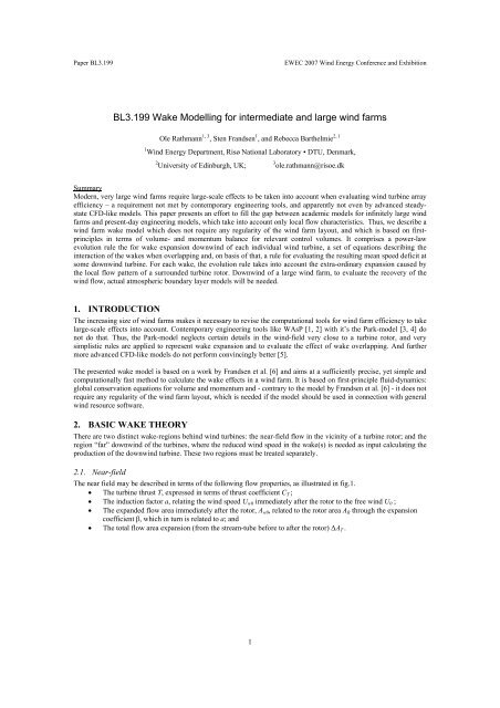
The near field may be described in terms of the following flow properties, as illustrated in fig.1.
• The turbine thrust T, expressed in terms of thrust coefficient C T ;
• The induction factor a, relating the wind speed U w0 immediately after the rotor to the free wind U 0 ;
• The expanded flow area immediately after the rotor, A w0 , related to the rotor area A R through the expansion
coefficient β, which in turn is related to a; and
• The total flow area expansion (from the stream-tube before to after the rotor) ΔA T .
1

Paper BL3.199
EWEC 2007 Wind Energy Conference and Exhibition
0.75
0.5
T
1
2
=
2
ρ C U (1)
T 0
0.25
0
-0.25
U 0
A R
T
A w0
U w0
Uw
A
w0
= (1 − a)
U (2) a = 1− 1− C (3)
T
0 0
= β A (4)
R
1
1−
2
a
β=
1−
a
(5)
-0.5
Δ A = A aβ (6)
T
R
-0.75
-2 -1 0 1 2
Figure 1. The near-field flow around a wind-turbine rotor.
2.2. The far-field
A cylindrical control volume is applied, aligned with the wind direction, containing all relevant turbines, and
sufficiently wide, so that the speed deficit in the wind direction is vanishingly small at the cylindrical surface.
U 0
U w
(y, z)
A
Figure 2. Cylindrical control volume around a set of turbines. In fact, the control volume should include a cut-off at the
ground level, but for graphical reasons this has been left out.
Disregarding large-scale pressure gradients and shear forces at the control volume surface, volume and momentum
balance equations for the control volume imply that the flow field U w (y,z) at some downwind position is related to the
sum of turbine thrusts by
1
( )
T = U ( y, z) U −U ( y, z)
dydz
∑ i ∫∫ (7)
A
w 0 w
ρ i
or expressed in terms of the relative speed deficit
1
U −U
U
w 0
δ≡ (8):
∑T = δ( y, z) ( 1 −δ( y, z)
) dydz
i ∫∫ (9)
2
A
ρU
0 i
Here the integration (y,z) is over the cross section of the exit area of the control volume.
0
2

Paper BL3.199
EWEC 2007 Wind Energy Conference and Exhibition
2.3. Turbulence
Turbulence within a wake is expected to have an impact on the wake expansion rate, and also to vary in response to the
wake expansion. However, an explicit treatment of turbulence intensity and it’s impact on wake behavior has been left
out to keep the present model sufficiently simple. The effect of turbulence will eventually be parameterized through the
wake expansion variables.
3. WAKE EXPANSION
The single-wake expansion model is based on the work by Frandsen [6]. The wake is assumed to have a circular cross
section. For a certain downwind cross section the true speed deficit profile is believed to be Gaussian-like. However,
Frandsen showed that essentially no generality would be lost if one approximates the speed deficit profile by a socalled
top-hat profile, and in the present model this approximation has been adopted:
1
⎧r ≤ 2 D ( x): ΔU ( x)
w
w ⎫
U − U ( x, r)
=
0 w ⎨
⎬
r
1
⎩ > 2 D ( x): 0
w ⎭
x: downwind distance from the rotor from which the wake originates
r: radial distance from the wake centerline defined by the centre of the rotor
(10)
i.e. a profile with an x-depending speed deficit inside the wake boundary, and zero outside.
The wake expansion rule of the present model is based on the power-law expansion suggested by Frandsen, but
extended to take into account the extra expansion occurring when passing a surrounded turbine rotor due to the nearfield
stream-line expansion occurring here, see Figure 1. Also, it has been taken into account that there are indications
that the wake diameter tends to zero when extrapolated back to its originating rotor [7].
1/ k
⎡ ⎛
k /2 x ⎞⎤
Dw( x) = DR
⎢max ⎜β , α ⎟⎥
Ψ
⎣ ⎝ DR
⎠⎦
Here α is of the order 1.0, k is between 2 and 3, and Ψ is a parameter or order unity which increases stepwise to account
for the “extra expansion” due to surrounded turbine rotors. The wake cross sectional area is then – including a cut-off
area at ground surface:
π
A ( ) ( ( )) 2
w
x = Dw x − ACut − off
(12)
4
(11)
The stepwise evolution of Ψ when passing a surrounded turbine “j” is governed by the following equation:
[ j] [ j−1]
Aw( xj, Ψ ) − Aw( xj, Ψ ) =Δ AT,
j
(13)
ΔA
( j) T,
j
[ j] [ j−1]
Φ = 1 + = A ( , )/ ( , )
[ j 1] w
xj Ψ Aw x
−
j
Ψ
A ( x , Ψ )
(14)
w
j
( j)
Here ΔA T,j is the stream-line area expansion around turbine “j” (eq. 6), and denotes the corresponding wake area
expansion ratio. Also, we introduce the relative increase in Ψ at turbine “j”, Ψ (j) , through
j
[ j] ( k )
Ψ = Ψ
∏ (15)
k = 1
Φ
3

Paper BL3.199
EWEC 2007 Wind Energy Conference and Exhibition
4. WAKE INTERACTION – Mosaic-tile model
The speed deficit distribution at some down-wind (turbine) position is approximated by a pattern of “mosaic tile”
regions, each with one or more overlapping wakes, and - in line with the top-hat profile for single wakes – with a
constant speed deficit. The principle is illustrated in figures 3A and 3B.
A 1
A 12
A 1
A 12
Wake 1
A 123
Wake 1
A 123
Wake 2
Wake 2
Wake 3
Wake 3
A 13
Affected rotor
Affected rotor
Ground
Ground
A. B.
Figure 3. Wake pattern examples.
From Eq.(9) one then get the following equation for the relative speed deficits for the tile regions, where the last
summation is over all tile regions J:
1
ρU
2
0
Nturbines
∑
i=
1
T
i
J∈( Tile regions)
∑
= A δ (1 −δ )
J
J J J
(16)
It should be noted that the symbol J denotes a set of indices for the wakes making up the tile region in question; thus in
figure 3.A, J would take the values [1] (wake 1 only), [1,2] (overlapping region of just wake 1 and 2) and [1,2,3]
(overlapping region of wakes 1, 2 and 3).
This equation is in fact rather complicated but it may be solved for each of the relative tile speed deficits δ J as follows:
a. Apply the equation recursively to any subgroup of the N turbines,
b. Take the relative speed deficit for so-called incomplete tiles (tiles partly cut off by another wake) to be identical to
those for the corresponding complete tiles, i.e. disregard other individual wakes than those defining the tile. E.g. in
fig 3.A, wake 3 is disregarded when calculating δ [12] and in fig.3.B wakes 2 and 3 are disregarded when
calculating δ [1] .
c. Step b. involves back-correcting for the extra wake expansion, due to the turbines thus disregarded through the Φ-
factors. This back-correction is accomplished by the use of effective tile areas A +(J) , related to the treatment of
each complete tile J.
For convenience we introduce the property ε J related to δ J by
2ε
1
ε ≡ δ (1 −δ ), δ = ½ −
4
−ε =
(17)
J J J
1+ 1−4ε
Then for a certain tile region J the relative speed deficit is found as:
Tile with a single wake i ( J = [i]) :
1
ρU
[] [] 2 i
i i
0
Tile with a set J of q overlapping wakes, q = Order(J)>1:
( q)
i∈J
q−1
1
ε ( q) ( q)
=
2 i −
J J
ρU
0 i r=
1
ε
A
+
=
T
∑ ∑ K J
( q )
⊂
+ + ( J )
∑ εK
K
( r )
K
A T A
The mean speed deficit δ (R) over the rotor area A (R) of a downwind rotor is then found as
n
( R) ( R)
( R)
A δ = ∑∑
A ( p) δ ( p)
J J
p=
1
J( p)
(18)
(19)
(20)
4

Paper BL3.199
EWEC 2007 Wind Energy Conference and Exhibition
where
( R)
A J denotes the part of the tile area overlapping with the rotor.
The effective tile areas A + are related to the true tile areas by the following equations, where
of tile K, i.e. the entire overlapping area of the wakes contained in the set K:
*
A K
denotes the gross area
with
q ⊂ ⊆
( q) ( q)
+ ( J ) * + ( J ) + ( )
( p) = ( p) ( p)
− ∑ K ∑
L J
J
K K K
L
( r )
r= p+
1 L
A A / Φ A , p < q
A 0 [ l > ∪ ]
+ ( J )
⎛
( l )
⎞
Φ = ∑⎜w / w,
w
i ∏ K
K
Φ =
i ⎟ ∑ i i
i∈K⎝
l∉J
⎠ i∈K
1
( A ( x))
i
* 2
(21)
(22)
5. TEST AGAINST WIND FARM DATA – STATUS.
The wake model has been tested against data from the Horns Rev offshore Wind Farm in the North Sea West of
Esbjerg – see the illustration of figures 4 and 5.
6152
Northing (km)
6151
6150
6149
WT01
WT02
WT03
WT04
270 deg.
WT11
WT12
WT13
WT14
WT21
WT22
WT23
WT24
WT31
WT32
WT33
WT34
WT41
WT42
WT43
WT44
WT51
WT52
WT53
WT54
WT61
WT62
WT63
WT64
WT71
WT72
WT73
WT74
WT81
WT82
WT83
WT84
WT91
WT92
WT93
WT94
WT05
WT06
WT15
WT16
WT25
WT26
WT35
WT36
WT45
WT46
WT55
WT56
WT65
WT66
WT75
WT76
WT85
WT86
WT95
WT96
Figure 4. Horns Rev Wind
Farm Layout.
• 80 Vestas 2MW turbines
• Rotor diameter: 80 m,
Hub height: 70m.
• Spacing: about 7 rotor
diameters.
WT07
WT17
WT27
WT37
WT47
WT57
WT67
WT77
WT87
WT97
6148
WT08
WT18
WT28
WT38
WT48
WT58
WT68
WT78
WT88
WT98
222 deg.
6147
423 424 425 426 427 428 429 430
Easting (km)
The wind directions along the main rows and the diagonal rows are indicated by arrows. Wind data with these
directions were used when comparing to model results.
Figure 5. Horns Rev Wind Farm. Aerial view.
5

Paper BL3.199
EWEC 2007 Wind Energy Conference and Exhibition
Data for wind directions 270 ° (Westerly wind) and 222 ° (South westerly wind), in line with the main-row and the
diagonal-row direction, respectively, were used as indicated in figure 4.
The results from a previous semi-linear version of the model have been compared to the wind farm data as shown in
figure 6. Whereas the speed deficit level is in agreement with data the semi-linear model-version was not able to
capture the details in the down-wind evolution of the speed deficit through the wind farm – also when varying the wake
expansion parameter α.
1.1
1
Relative Speed
0.9
0.8
0.7
0.6
0.5
Alfa=0.7
Meas.
Alfa=1.0
Alfa=0.7
Meas.
Alfa=0.5
0.4
0 10 20 30 40 50 60
0 20 40 60
Wind direction: 270°+/-1° Wind direction: 222°+/-2°
Free wind speed 9 m/s +/- 0.5 m/s.
Free wind speed: 9 m/s +/- 1 m/s
Figure 6. Comparison with results from semi-linear version of the model.
Results from the present model for an intermediate (8.5 m/s) and for a high wind speed (12 m/s) are presented in
figures 7 and 8.
9
Reduced wind speed (m/s)
8
7
Row 4 (middle)
Case A.1
Data
Model Pred.
Row 8 (southern)
6
0 2000 4000 6000
Downwind distance (m)
2000 4000 6000
Reduced wind speed (m/s)
12
11
10
9
Row 4 (middle)
Case A.3
Data
Model Pred.
Row 8 (southern)
0 2000 4000 6000
Downwind distance (m)
Figure 7. Model predictions at wind direction 270° +/-3° compared to data.
Free wind speed: 8.5 m/s +/- 0.5 m/s (top) and 12.0 m/s +/- 0.5 m/s (bottom).
2000 4000 6000
6

Paper BL3.199
EWEC 2007 Wind Energy Conference and Exhibition
9
Reduced wind speed (m/s)
8
7
Row 8 (middle diag.)
Case C.1
Data
Model Pred.
Row 10 (eastern diag.)
6
0 2000 4000 6000
Downwind distance (m)
2000 4000 6000
Reduced wind speed (m/s)
12
11
10
9
Row 8 (middle diag.)
Case C.3
Data
Model Pred.
Row 10 (eastern diag.)
0 2000 4000 6000
Downwind distance (m)
2000 4000 6000
Figure 8. Model predictions at wind direction 222° +/-3° compared to data.
Free wind speed: 8.5 m/s +/- 0.5 m/s (top) and 12.0 m/s +/- 0.5 m/s (bottom).
This allows to see whether the comparison differ in any principal way due to the somewhat smaller turbine thrust at
high wind speed. For both wind directions the comparison were performed for a central row of turbines (where wake
overlapping from both sides may occur) and a row located at the boundary (with wake overlapping from only one side).
Clearly, the model is not able to predict the details in the observed downwind evolution of the speed deficit. The high
wind speed case is not different in this respect from the intermediate wind speed. The discrepancy is especially evident
for wind direction 270° where the predicted speed deficit continues to increase in contradiction to the measured data
which levels out after a few downwind turbine positions. It is obvious to attribute this discrepancy to improper values
of the wake parameters k and α in response to wind conditions and wake overlapping.
6. DISCUSSION
• The wind speed deficit at the first wake-effected turbine is generally predicted well;
• The new “mosaic tile” model - with the selected wake expansion parameters - seems to be able to yield a
somewhat better prediction than the previous semi-linear model .
• The new model still does not reach a stationary reduced speed - as seen in the data.
• The wake expansion parameters may have to depend on the degree of local wake-interaction.
7. DOWNWIND REGION
The region downwind of large wind farms cannot be expected to be treatable by wake models since the wakes will
typically have developed to a size where interaction with the atmospheric boundary layer starts to take place. Also, the
turbulence level will be rather high and may lead to faster wind speed recovery than expected from single- or multiple
wake considerations.
Instead, it is suggested that flow models for the atmospheric boundary layer may be used, possibly with the output from
the present wake model serving as an inflow-condition.
7

Paper BL3.199
EWEC 2007 Wind Energy Conference and Exhibition
8. CONCLUSION
• The new “mosaic tile” model seems promising, and is believed to be able to be developed to an efficient tool for
estimating wake effects in large wind farms.
• The algorithm is in its present form is too time consuming; more efficient methods to calculate the wake tile areas
must be developed.
• By comparison with more wind farm data, optimal values for the wake expansion parameters k and α must be
found, including dependence on local wake interaction conditions.
• For the far-field region downwind of a wind farm the “mosaic tile” wake model may be combined with boundary
layer models to treat this region separately.
9. REFERENCES
[1] I.Troen, E.L. Petersen: European Wind Atlas. Risø National Laboratory 1989.
[2] N.G.Mortensen, D.N.Heathfield, L.Myllerup, L.Landberg, O.Rathmann, I.Troen and E.L.Petersen: Getting Started
With WAsP8. Risø National Laboratory 2003 (Risø-I-1950(EN) ).
[3] N.O.Jensen, A Note on Wind Generator Interaction, Risoe National Laboratory 1983. (Risoe-M-2411)
[4] I. Katic, J. Højstrup and N.O.Jensen, A Simple Model for Cluster Efficiency. Proceedings of European Wind
Energy Conference and Exhibition, Rome, 1986; 407-410.
[5] R.J.L. Barthelmie et al., Comparison of Wake Model Simulations with Off-shore Wind Turbine Wake Profiles
Measured by Sodar. Journal of Atmospheric and Oceanic Technology.
[6] S. Frandsen et al., Analytical Modeling of Wind speed Deficit in Large Offshore Wind Farms, Wind Energy 9, 39-
53 (2006).
[7] R.J.Barthelmie, S.T.Frandsen, P.-E.Rethore, M.Mechali, S.C.Pryor, L.Jensen and P.Sørensen, Modelling and
Measurements of Offshore Wakes. Owemes 2006 Conference, 20-22 April, Citavecchia, Italy.
10. ACKNOWLEDGEMENT
This work has been financed
• by the Danish Public Service Obligation (PSO) funds (F&U 4103),
• by the Danish Strategic Council of Research, and
• by the EU Upwind Project (ref. SES6 019945), work package 8.
Data from Horns Rev wind farm were provided by Elsam Engineering and DONG Energy.
Thanks are due to Pierre-Elouan Rethore for extracting the specific Horns Rev data used in this work.
8