Chapter 5 Urban Area Travel Demand Model - Saginaw County
Chapter 5 Urban Area Travel Demand Model - Saginaw County
Chapter 5 Urban Area Travel Demand Model - Saginaw County

You also want an ePaper? Increase the reach of your titles
YUMPU automatically turns print PDFs into web optimized ePapers that Google loves.
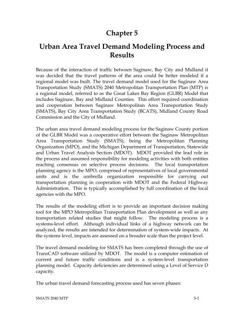
<strong>Chapter</strong> 5<br />
<strong>Urban</strong> <strong>Area</strong> <strong>Travel</strong> <strong>Demand</strong> <strong>Model</strong>ing Process and<br />
Results<br />
Because of the interaction of traffic between <strong>Saginaw</strong>, Bay City and Midland it<br />
was decided that the travel patterns of the area could be better modeled if a<br />
regional model was built. The travel demand model used for the <strong>Saginaw</strong> <strong>Area</strong><br />
Transportation Study (SMATS) 2040 Metropolitan Transportation Plan (MTP) is<br />
a regional model, referred to as the Great Lakes Bay Region (GLBR) <strong>Model</strong> that<br />
includes <strong>Saginaw</strong>, Bay and Midland Counties. This effort required coordination<br />
and cooperation between <strong>Saginaw</strong> Metropolitan <strong>Area</strong> Transportation Study<br />
(SMATS), Bay City <strong>Area</strong> Transportation Study (BCATS), Midland <strong>County</strong> Road<br />
Commission and the City of Midland.<br />
The urban area travel demand modeling process for the <strong>Saginaw</strong> <strong>County</strong> portion<br />
of the GLBR <strong>Model</strong> was a cooperative effort between the <strong>Saginaw</strong> Metropolitan<br />
<strong>Area</strong> Transportation Study (SMATS), being the Metropolitan Planning<br />
Organization (MPO), and the Michigan Department of Transportation, Statewide<br />
and <strong>Urban</strong> <strong>Travel</strong> Analysis Section (MDOT). MDOT provided the lead role in<br />
the process and assumed responsibility for modeling activities with both entities<br />
reaching consensus on selective process decisions. The local transportation<br />
planning agency is the MPO, comprised of representatives of local governmental<br />
units and is the umbrella organization responsible for carrying out<br />
transportation planning in cooperation with MDOT and the Federal Highway<br />
Administration. This is typically accomplished by full coordination of the local<br />
agencies with the MPO.<br />
The results of the modeling effort is to provide an important decision making<br />
tool for the MPO Metropolitan Transportation Plan development as well as any<br />
transportation related studies that might follow. The modeling process is a<br />
systems-level effort. Although individual links of a highway network can be<br />
analyzed, the results are intended for determination of system-wide impacts. At<br />
the systems level, impacts are assessed on a broader scale than the project level.<br />
The travel demand modeling for SMATS has been completed through the use of<br />
TransCAD software utilized by MDOT. The model is a computer estimation of<br />
current and future traffic conditions and is a system-level transportation<br />
planning model. Capacity deficiencies are determined using a Level of Service D<br />
capacity.<br />
The urban travel demand forecasting process used has seven phases:<br />
SMATS 2040 MTP 5-1
1. Data Collection, in which socio-economic and facility inventory data are<br />
collected.<br />
2. Trip Generation, which calculates the number of person trips produced in or<br />
attracted to a traffic analysis zone (TAZ).<br />
3. Trip Distribution, which takes the person trips produced in a TAZ and<br />
distributes them to all other TAZs, based on attractiveness of the zone.<br />
4. Mode Choice, which assigns person trips to a mode of travel such as drive<br />
alone, shared ride 2, shared ride 3+, walk to transit, park and ride transit.<br />
5. Assignment, which determines what routes are utilized for trips. There is a<br />
highway assignment and a transit assignment.<br />
6. <strong>Model</strong> Calibration/Validation, which is performed at the end of each<br />
modeling step to make sure that the results from that step are within<br />
reasonable ranges. The final assignment validation involves verifying that<br />
the volumes (trips) estimated in the base year traffic assignment replicate<br />
observed traffic counts.<br />
7. System Analysis, tests alternatives and analyzes changes in order to<br />
improve the transportation system.<br />
There are two basic systems of data organization in the travel demand<br />
forecasting process. The first system of data is organized based on the street<br />
system. Roads with a national functional class (NFC) designation of "minor<br />
collector" and higher are included in the network. Some local roads are included<br />
to provide connectivity in the network or because they were deemed regionally<br />
significant. The unit of analysis is called a "link." Usually, a link is a segment of<br />
roadway which is terminated at each end by an intersection. In a traffic<br />
assignment network, intersections are called "nodes." Therefore, a link has a<br />
node at each end.<br />
The second data organization mechanism is the Traffic Analysis Zones (TAZ).<br />
TAZs are determined based upon several criteria, including similarity of land<br />
use, compatibility with jurisdictional boundaries, the presence of physical<br />
boundaries, and compatibility with the street system. Streets are generally<br />
utilized as zone boundary edges. All socio-economic and trip generation<br />
information for both the base year and future year are summarized by TAZ. The<br />
Traffic Analysis Zones used for model development are depicted on a series of<br />
maps that are on file with the MPO and available for viewing at the SMATS<br />
office. They have not been reproduced here due to space limitations.<br />
SMATS 2040 MTP 5-2
The two data systems, the street system (network) and the TAZ system (socioeconomic<br />
data), are interrelated through the use of "centroids." Each TAZ is<br />
represented on the network by a point (centroid) which represents the weighted<br />
center of activity for that TAZ. A centroid is connected by a set of links to the<br />
adjacent street system. That is, the network is provided with a special set of links<br />
for each TAZ which connects the TAZ to the street system. Since every TAZ is<br />
connected to the street system by these "centroid connectors,” it is possible for<br />
trips from each zone to reach every other zone by way of a number of paths<br />
through the street system.<br />
Network<br />
A computerized "network" (traffic assignment network) is built to represent the<br />
existing street system. The GLBR <strong>Model</strong> network is based on the Michigan<br />
Geographic Framework version 10 and includes most streets within the study<br />
area classified as a "minor collector" or higher by the national functional<br />
classification system. Other roads are added to provide continuity and/or allow<br />
interchange between these facilities.<br />
Transportation system information or network attributes required for each link<br />
include facility type, area type, lane width, number of through lanes, parking<br />
available, national functional classification, traffic counts (where available), and<br />
volumes for level of service D (frequently described as its capacity). If the<br />
information is not the same for the entire length of a link, the predominant value<br />
is used. The network attributes were provided to the MPO and MDOT staff by<br />
the respective road agencies, with the exclusion of link capacity. The link<br />
capacity was determined by utilizing the Capacity Calculator program which<br />
takes into account the network attributes and sets a capacity that would<br />
approximate a level of service “D” or acceptable level of traffic. Higher volume<br />
to capacity ratios are characterized by: stop-and–go-travel, reduced flow rates<br />
and severe intersection delays. This typifies unacceptable or deficient traffic<br />
conditions.<br />
The street network is used in the traffic assignment process. The traffic<br />
assignment process takes the trip interactions between zones from trip<br />
distribution and loads them onto the network. The travel paths for each zone-tozone<br />
interchange are based on the minimum travel time between zones. They<br />
are calculated by a computer program which examines all possible paths from<br />
each origin zone to all destination zones. The shortest path is determined by the<br />
distance of each link and the speed at which it operates. The program then<br />
calculates travel times for all of the possible paths between centroids and records<br />
the links which comprise the shortest travel time path.<br />
SMATS 2040 MTP 5-3
The transit network is used in the transit assignment process and overlays the<br />
street network as a route system. It reflects the current fixed route system<br />
available for the base year. It has its own set of attributes such as bus headway,<br />
speed and rider fee. Person trips that are determined to be transit trips are<br />
assigned to this network.<br />
Speeds used to calculate minimum travel times are based on each link's national<br />
functional classification, facility type, and area type. Speeds represent a relative<br />
impedance to travel and not posted speed limits.<br />
Socio-Economic Data<br />
<strong>Travel</strong> demand models are driven, in part, by the relationship of land use<br />
activities and characteristics to the transportation network. Specific inputs to the<br />
modeling process are land use activity including the number of households,<br />
population-in-households, vehicles, and employment located in a given<br />
transportation analysis zone (TAZ). The modeling process translates this data<br />
into vehicle trips on the modeled transportation network. Socio-Economic data<br />
were developed for the 2009 base year and for the 2020, 2030 and 2040 forecast<br />
years.<br />
It is important to remember that socio-economic forecasting is essentially a<br />
matter of judgment. Judgment is required in selecting the type of forecast to be<br />
implemented; in determining the procedures for making the forecast; and, the<br />
process used in reviewing the effects of the factors that induce changes in<br />
population and employment. The establishment of a large new industry or the<br />
loss of a similar size industry can lead to considerable impact on an area’s<br />
development.<br />
Therefore, although socio-economic projections are a useful and required tool in<br />
the planning of an area’s future growth and development, it is important to note<br />
that the projections are not infallible and should be modified as time progresses<br />
to better reflect development impacts occurring in the SMATS planning area.<br />
The TAZ’s were created from the 2000 census blocks and constrained by the<br />
network and Minor Civil Division (MCD) boundaries. Values for population<br />
and occupied households were aggregated from the 2000 census blocks to arrive<br />
at TAZ totals for 2000. MPO staff used this and MCD projections as well as input<br />
from local officials to develop the TAZ values for the base year of 2009 and<br />
forecast years of, 2020, 2030 and 2040.<br />
Employment data was obtained from the combination of the Michigan<br />
Employment Security Commission (MESC), and the propriety databases<br />
SMATS 2040 MTP 5-4
available from Claritas (2008 Business Point Data) and Hoovers (business address<br />
file). The resulting database was reviewed locally. The employment data for<br />
2009, 2020, 2030 and 2040 were developed using growth rates based on the REMI<br />
(Regional Econometric, Inc.) projections as well as local knowledge of expected<br />
development.<br />
SMATS staff and committees reviewed the estimates and projections and made<br />
adjustments given their local knowledge and greater understanding of the<br />
unique local circumstances in each TAZ.<br />
Trip Generation<br />
The trip generation process calculates the number of person-trips produced from<br />
or attracted to a zone, based on the socio-economic characteristics of that zone.<br />
The urban transportation forecasting models do not consider travel<br />
characteristics such as direction, length, or time of occurrence as part of trip<br />
generation. The relationship between person-trip making and land activity are<br />
expressed in equations for use in the modeling process. The formulas were<br />
derived from MI <strong>Travel</strong> Counts Michigan travel survey data and other research<br />
throughout the United States. Productions were generated with a crossclassification<br />
look-up process based on household demographics. Attractions<br />
were generated with a regression approach based on employment and<br />
household demographics. In order to develop a trip table, productions (P's) and<br />
attractions (A's) must be balanced also referred to as normalization.<br />
The GLBR travel demand model also has a simple truck model that estimates<br />
commercial and heavy truck traffic based on production and attraction<br />
relationships developed from the Quick Response Freight Manual I (QRFM I).<br />
The QRFM I uses the employment data from the TAZs in its calculations.<br />
Trips that begin or end beyond the study area boundary are called "cordon trips."<br />
These trips are made up of two components: external to internal (EI) or internal<br />
to external (IE) trips and through-trips (EE). EI trips are those trips which start<br />
outside the study area and end in the study area. IE trips start inside the study<br />
area and end outside the study area. EE trips are those trips that pass through<br />
the study area without stopping; this matrix is referred to as the through-trip<br />
table.<br />
Trip Distribution<br />
Trip distribution involves the use of mathematical formula which determines<br />
how many of the trips produced in a zone will be attracted to each of the other<br />
zones. It connects the ends of trips produced in one zone to the ends of trips<br />
attracted to other zones. The equations are based on travel time between zones<br />
SMATS 2040 MTP 5-5
and the relative level of activity in each zone. Trip purpose is an important<br />
factor in development of these relationships. The trip relationship formula<br />
developed in this process is based on principals and algorithms commonly<br />
referred to as the Gravity <strong>Model</strong>.<br />
The process which connects productions to attractions is called trip distribution.<br />
The most widely used and documented technique is the "gravity model" which<br />
was originally derived from Newton's Law of Gravity. Newton's Law states that<br />
the attractive force between any two bodies is directly related to the masses of<br />
the bodies and inversely related to the distance between them. Analogously, in<br />
the trip distribution model, the number of trips between two areas is directly<br />
related to the level of activity in an area (represented by its trip generation) and<br />
inversely related to the distance between the areas (represented as a function of<br />
travel time).<br />
Research has determined that the pure gravity model equation does not<br />
adequately predict the distribution of trips between zones. In most models the<br />
value of time for each purpose is modified by an exponentially determined<br />
"travel time factor" or "F factor" --also known as a "Friction Factor." "F factors"<br />
represent the average area-wide effect that various levels of travel time have on<br />
travel between zones. The "F factors" used were developed using an exponential<br />
function described in the <strong>Travel</strong> Estimation Techniques for <strong>Urban</strong> Planning,<br />
NCHRP 365. The matrix is generated in TransCAD during the gravity model<br />
process.<br />
The primary inputs to the gravity model are the normalized productions (P’s)<br />
and attractions (A's) by trip purpose developed in the trip generation phase. The<br />
second data input is a measure of the temporal separation between zones. This<br />
measure is an estimate of travel time over the transportation network. Zone-tozone<br />
travel times are referred to as "skims."<br />
In order to more closely approximate actual times between zones and also to<br />
account for the travel time for intra-zonal trips, the skims were updated to<br />
include terminal and intra-zonal times. Terminal times account for the nondriving<br />
portion of each end of the trip and were generated from a look-up table<br />
based on area type. They represent that portion of the total travel time used for<br />
parking and walking to the actual destination. Intra-zonal travel time is the time<br />
of trips that begin and end within the same zone. Intra-zonal travel times were<br />
calculated utilizing a nearest neighbor routine.<br />
The Gravity <strong>Model</strong> utilizes the by-purpose P’s & A's, the by-purpose "F factors",<br />
and the travel times, including terminal and intra-zonal.<br />
SMATS 2040 MTP 5-6
Mode Choice<br />
The number of person trips and their trip starting and ending point have been<br />
determined in the trip generation and trip distribution steps. The mode choice<br />
step determines how each person trip will travel. The GLBR travel demand<br />
model uses a nested logit model to predict mode choice.<br />
With this logit structure the basic modes are:<br />
1. Single Occupancy Vehicle (SOV)<br />
2. Shared Ride 2 people in vehicle (SR2)<br />
3. Shared Ride 3 or more people in vehicle (SR3+)<br />
4. Walk to transit stop<br />
5. Drive to transit stop<br />
Mode choice model utility equations are used to predict the mode used for a trip.<br />
Utility equations vary by trip type and take into consideration things like invehicle<br />
time, out-of-vehicle time, length and cost. The proximity to transit routes<br />
or park and ride locations limits the TAZs that can utilize transit options. The<br />
output to this step is a vehicle trip matrix and transit trip matrix. The external<br />
trips and the truck trips are added to the vehicle trip matrix.<br />
Assignment<br />
The GBLR model has 4 time periods that were developed to match the peak<br />
periods observed in traffic counts.<br />
The following period were used:<br />
AM Peak (7a - 9a)<br />
Mid Day (9a - 3p)<br />
PM Peak (3p - 6p)<br />
Night Time (6p – 7a)<br />
A fixed time of day factor method was utilized. The factors were developed<br />
from the MI <strong>Travel</strong> Counts Michigan travel survey data and vary by trip type.<br />
Default factors from the Quick Response Freight Manual I (QRFM I) were used<br />
for truck trips.<br />
SMATS 2040 MTP 5-7
The traffic assignment process takes the trips produced in a zone (trip<br />
generation) and distributed to other zones (trip distribution) and loads them<br />
onto the network via the centroid connectors. A program examines all of the<br />
possible paths from each zone to all other zones and calculates all reasonable<br />
time paths from each zone (centroid) to all other zones. Trips are assigned to<br />
paths that are the shortest path between each combination of zones. As the<br />
volumes assigned to links approach capacity, travel times on all paths are<br />
recalculated to reflect the congestion and the remaining trips are assigned to the<br />
next shortest path. This process continues through several iterations until no trip<br />
can reduce its travel time by taking the next shortest path. This is a user<br />
equilibrium assignment method and reflects the alternative routes that motorists<br />
use as the shortest path becomes congested. The assignment produces an<br />
assigned volume for each link.<br />
The transit assignment is a daily assignment and uses the transit network route<br />
system to assign the shortest path for trips.<br />
<strong>Model</strong> Calibration/Validation<br />
The outputs of each of the four main steps, Trip Generation, Trip distribution,<br />
Mode Choice and Assignment, are checked for reasonableness against national<br />
standards. Modifications can be made at each step before moving on to the next.<br />
The final model calibration/validation verifies that the assigned volumes<br />
simulate actual traffic counts on the street system. When significant differences<br />
occur, additional analysis is conducted to determine the reason. At this time<br />
additional modifications may be made to the network speeds and configurations<br />
(hence paths), trip generation (special generators), trip distribution (F factors),<br />
socio-economic data, or traffic counts.<br />
The purpose of this model calibration phase is to verify that the base year<br />
assigned volumes from the traffic assignment model simulate actual base year<br />
traffic counts. When this step is completed, the systems model is considered<br />
statistically acceptable. This means that future socio-economic data or future<br />
network capacity changes can be substituted for base (existing) data. The trip<br />
generation, trip distribution, mode choice and traffic assignment steps can be<br />
repeated, and future trips can be estimated for systems analysis. It is assumed<br />
that the quantifiable relationships modeled in the base year will remain<br />
reasonably stable over time.<br />
Applications of the Calibrated/Validated <strong>Model</strong><br />
Forecasted travel is produced by substituting forecasted socio-economic and<br />
transportation system data for the base year data. This forecasted data is<br />
SMATS 2040 MTP 5-8
provided by the MPO. The same mathematical formulae are used for the base<br />
and future year data. The assumption is made that the relationships expressed<br />
by the formulae in the base year will remain constant over time (to the target<br />
date).<br />
After either base year or future trips are simulated, other types of modeling<br />
studies can be conducted.<br />
• Network alternatives to relieve congestion can be tested for the 2040<br />
Metropolitan Transportation Plan. Future traffic can be assigned to the<br />
existing network to show what would happen in the future if no<br />
improvements were made to the present transportation system. This<br />
process is often referred to as "deficiency analysis." From this,<br />
improvements can be planned that would alleviate demonstrated capacity<br />
problems.<br />
• The impact of planned roadway improvements or network changes can be<br />
assessed.<br />
• Links can be analyzed to determine what zones are contributing to the<br />
travel on that link. This can be shown as a percentage breakdown of total<br />
link volume.<br />
• The network can be tested to simulate conditions with or without a<br />
proposed bridge or new road segment. The assigned future volumes on<br />
adjacent links would then be compared to determine traffic flow impacts.<br />
This, in turn, would assist in assessing whether the bridge should be<br />
replaced and/or where it should be relocated.<br />
• Road closure/detour evaluation studies can be conducted to determine<br />
the effects of closing a roadway. This type of study is very useful for<br />
construction management.<br />
• The impacts of land use changes on the network can also be evaluated<br />
(e.g., what are the impacts of a new regional mall being built).<br />
Two issues are critical in using the modeling tools and processes:<br />
• The modeling process is most effective for system level analysis.<br />
Although detailed volumes for individual intersection and "links" of a<br />
highway are an output of the model, additional analysis and modification<br />
of the model output may be required for project level analysis.<br />
• The accuracy of the model is heavily dependent on the accuracy of the<br />
SMATS 2040 MTP 5-9
socio-economic data and network data provided by the local participating<br />
agencies, and the skill of the users in interpreting the reasonableness of<br />
the results.<br />
System Analysis for MTP<br />
Generally three different alternative scenarios are developed for the Long Range<br />
Transportation Plan:<br />
1. Existing trips on the existing system. This is the "calibrated," existing<br />
network/scenario. This is a prerequisite for the other two scenarios.<br />
2. Future trips on the existing network. Future trips are assigned to the<br />
existing network. This alternative displays future capacity and congestion<br />
problems if no improvements to the system are made. This is called the<br />
"No Build" alternative, and usually includes the existing system, plus any<br />
projects which are committed to be built in the future.<br />
3. Future trips on the future system. This scenario is the future Metropolitan<br />
Transportation Plan network. It includes capacity projects listed in the<br />
MTP.<br />
It is important to remember that the volume to capacity ratio reflects a volume<br />
for a specified time period and a capacity for that same period of time. It does<br />
not reflect deficiencies that only occur briefly at certain short time periods or<br />
because of roadway geometrics, or roadway condition.<br />
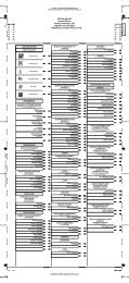
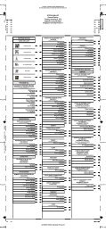
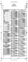
A series of maps was developed to display system deficiencies for the 2009 base<br />
year, 2040 with no capacity projects built, and 2040 with the capacity projects<br />
identified in the plan. For each scenario, separate maps were generated for each<br />
of the time periods considered: A.M. Peak, Mid-Day, P.M. Peak, and Night.<br />
Electronic copies of the full set of maps are on file with the MPO. To keep the<br />
electronic plan document a reasonable size, only the daily deficiency maps are<br />
included at the end of this chapter. These maps are composites that include the<br />
deficiencies from all the time periods on a single map for the 2009, 2040 “no<br />
build” and 2040 “build” scenarios. Finally, the deficiencies identified in the<br />
modeling process are also listed in Table 5-1.<br />
SMATS 2040 MTP 5-10
Table 5-1. Great Lakes Bay Region <strong>Travel</strong> <strong>Demand</strong> <strong>Model</strong><br />
<strong>Saginaw</strong> <strong>County</strong> Capacity Deficiencies<br />
February 9, 2012<br />
2009 V/C<br />
with TIP<br />
Projects<br />
2040 V/C<br />
without MTP<br />
Projects<br />
2040 V/C<br />
with MTP<br />
Projects<br />
Road Name<br />
Extent<br />
Am Peak (7a-9a)<br />
Miller Road State to Gratiot 1 - 1.17 1.1 - 1.34 Not Deficient<br />
Dixie Highway Airport to Junction .81 - 1.14 .82 - 1.19 .82- 1.19<br />
Main Street Maple to I-75 .77 - 1.04 .81 - 1.06 .81 - 1.06<br />
Gratiot Midland to St. Andrews Not Deficient .66 - 1.01 .66 - 1.01<br />
Gratiot Golfview to Wheeler Not Deficient .7 - 1.03 .7 - 1.03<br />
Michigan Shattuck to Weiss Not Deficient .83 - 1.07 Not Deficient<br />
McCarty Lawndale to Mackinaw Not Deficient .62 - 1.13 .62 - 1.13<br />
Tittabawassee Center to Bay Not Deficient .45 - 1.12 .45 - 1.12<br />
Mid day (9a-3p)<br />
Miller Road State to Gratiot 1.05 - 1.06 .98 - 1.19 .98 - 1.19<br />
PM Peak (3p-6p)<br />
Miller Road State to Gratiot 1.04 - 1.19 1.14 - 1.28 Not Deficient<br />
Dixie Highway Airport to Portsmouth .87 - 1.02 .9 - 1.07 .9 - 1.07<br />
Michigan Shattuck to Weiss Not Deficient .69 - 1.14 .69 - 1.14<br />
McCarty Hemmeter to Mackinaw Not Deficient .73 - 1.06 .73 - 1.06<br />
Night (6p - 7a)<br />
None<br />
Daily<br />
Miller Road State to Gratiot 1.12 - 1.16 1.18 - 1.22 Not Deficient<br />
Dixie Highway Airport to Portsmouth 1.08 - 1.1 1.12 - 1.14 1.12 - 1.14<br />
Main Street Maple to I-75 Not Deficient 1.12 - 1.13 1.12 - 1.13<br />
Michigan Shattuck to Weiss Not Deficient .79 - 1.12 Not Deficient<br />
McCarty Hemmeter to Mackinaw Not Deficient 1 - 1.05 1 - 1.05<br />
SMATS 2040 MTP 5-11
Vassar<br />
King<br />
Gera<br />
Townline<br />
Junction<br />
Block<br />
Gera<br />
Fergus<br />
Fergus<br />
Birch Run<br />
Washington<br />
Holland<br />
Reimer<br />
Curtis<br />
Busch<br />
N I 75<br />
Dixie<br />
S I 75<br />
Portsmouth<br />
N I 75<br />
Sheridan<br />
Williamson<br />
Washington<br />
Airport<br />
Portsmouth<br />
1.1<br />
1.08<br />
Dixie<br />
Blackmar<br />
S I 75<br />
East<br />
Busch<br />
Sheridan<br />
Rathbun<br />
Seymour<br />
Morseville<br />
Birch Run<br />
Stroebel<br />
1.16<br />
1.16<br />
1.15 1.12<br />
1.15 1.12<br />
Gratiot<br />
Moore<br />
Curtis<br />
Morrish<br />
Albee<br />
Midland<br />
State<br />
River<br />
Miller<br />
Kennely<br />
Swan Creek<br />
Sharon<br />
Graham<br />
Frost<br />
Geddes<br />
Schomaker<br />
Gleaner<br />
Ederer<br />
Lakefield<br />
Genesee<br />
Tuscola<br />
Main<br />
Dehmel<br />
Maple<br />
Carrollton<br />
S I 675<br />
Hermansau<br />
Fashion Squa<br />
Bay<br />
Wadsworth<br />
Janes<br />
Niagara<br />
S I 75<br />
Towerline<br />
Hess<br />
Treanor<br />
King<br />
Baker<br />
Fort<br />
Bell<br />
Sloan<br />
Verne<br />
Bueche<br />
Hemmeter<br />
Lawndale<br />
Weiss<br />
Brockway<br />
Center<br />
Saint Andrews<br />
Michigan<br />
Graham<br />
Townline<br />
Shattuck<br />
N I 675/Davenport<br />
N I 75/N I 675<br />
Carroll<br />
N I 675<br />
Johnson<br />
Lapeer<br />
15th<br />
Harrison<br />
Hamilton<br />
Woodbridge<br />
Bond<br />
Malzahn<br />
N I 75/Holland<br />
S I 75/Holland<br />
Rust<br />
State<br />
N I 75/Dixie<br />
S I 75/Dixie<br />
Thistle<br />
North<br />
Main<br />
Outer<br />
W I 675/Veterans Memorial<br />
Erie<br />
Perkins<br />
Jefferson<br />
Birch Run/N I 75<br />
Birch Run/S I 75<br />
N I 75/Washington<br />
Mackinaw<br />
Ethel<br />
Genesee<br />
Webber<br />
Gallagher<br />
Thayer East<br />
Dayton<br />
Washington<br />
Norman<br />
Veterans Memorial<br />
Findley<br />
5th<br />
Blackmore<br />
Morson<br />
Warwick<br />
Davenport<br />
Mason<br />
Carolina<br />
Hill<br />
Stark<br />
McEwan<br />
Cooper<br />
12th<br />
14th<br />
Alexander<br />
Court<br />
21st<br />
Wright<br />
Cumberland<br />
17th<br />
Atwater<br />
Remington<br />
Bagley<br />
Gratiot<br />
Congress<br />
3rd<br />
Clinton<br />
Cherry<br />
Walnut<br />
Hoyt<br />
Howard<br />
Warren<br />
Ezra Rust<br />
Elm<br />
Fordney<br />
Williams<br />
Marquette<br />
Morris<br />
Great Lakes Bay Region <strong>Model</strong><br />
<strong>Saginaw</strong> <strong>County</strong><br />
2009 Network With TIP Projects<br />
2009 Daily Capacity Deficiencies<br />
Capacity Set At Level Of Service D<br />
February 9, 2012<br />
Map layers<br />
Water<br />
<strong>County</strong> Boundary<br />
2009 GLBR Network<br />
V/C 1 to 1.19<br />
El<br />
EB/WB M 81<br />
State/S I 675<br />
19th<br />
Jefferson<br />
McCoskry<br />
Vermont<br />
Wheeler<br />
Farmer<br />
Robinwood<br />
Owen<br />
Holmes<br />
River View<br />
Marshall<br />
Railroad<br />
East/Verne Cutoff<br />
Bueche/Verne Cutoff<br />
Nic<br />
incoln/Birch Run<br />
Wieneke<br />
Hospital<br />
N Midland/M 58 Bypass<br />
Gasper<br />
Thomas<br />
<strong>Saginaw</strong><br />
Chesaning<br />
Belle<br />
Ring<br />
Graham<br />
Walnut<br />
Orr<br />
Orr
Townline<br />
Fergus<br />
Bay<br />
Tuscola<br />
N I 75/Bay City<br />
Westervelt<br />
Adams<br />
Trautner<br />
Sherman<br />
ms/S I 75<br />
Portsmouth<br />
1.05<br />
1<br />
S I 75<br />
Veterans Memorial<br />
Carrollton<br />
1<br />
Washington<br />
1.11<br />
0.79<br />
Vassar<br />
Holland<br />
Stroebel<br />
N I 75<br />
King<br />
Gera<br />
Reimer<br />
Portsmouth<br />
1.14<br />
1.12<br />
Dixie<br />
Junction<br />
Blackmar<br />
S I 75<br />
Curtis<br />
East<br />
Busch<br />
Sheridan<br />
N I 75<br />
Rathbun<br />
Seymour<br />
Gera<br />
Dixie<br />
Morseville<br />
1.13<br />
1.12<br />
1.22 1.18<br />
1.22 1.18<br />
Swan Creek<br />
Sharon<br />
Ring<br />
Fordney<br />
Ithaca<br />
Birch Run<br />
River<br />
Gratiot<br />
Moore<br />
Curtis<br />
Morrish<br />
Birch Run<br />
Midland<br />
State<br />
McCarty<br />
Schust<br />
N I 675/Tittabawassee<br />
Davis<br />
Tittabawassee<br />
Mackinaw<br />
Center<br />
Lawndale<br />
Taylor<br />
Barnard<br />
Mapleridge<br />
N I 675<br />
S I 675<br />
Fashion Square<br />
Bay<br />
Shattuck<br />
Hemmeter<br />
N I 675/Davenport<br />
Weiss<br />
Wadsworth<br />
Lapeer<br />
Janes<br />
15th<br />
Niagara<br />
Woodbridge<br />
Malzahn<br />
Brockway<br />
Thistle<br />
Towerline<br />
N I 75/Holland<br />
S I 75/Holland<br />
Hamilton<br />
Rust<br />
Saint Andrews<br />
Hess<br />
Michigan<br />
Treanor<br />
Sheridan<br />
King<br />
Williamson<br />
Baker<br />
Washington<br />
Airport<br />
S I 75/Dixie<br />
State<br />
Genesee<br />
Fort<br />
Tuscola<br />
Dehmel<br />
Bell<br />
Sloan<br />
Maple<br />
Verne<br />
Albee<br />
Bueche<br />
Hospital<br />
Miller<br />
Frost<br />
Kennely<br />
Tittabawassee<br />
Graham<br />
Geddes<br />
Schomaker<br />
Graham<br />
North<br />
McLeod<br />
N I 75/Washington<br />
Outer<br />
S I 675/N I 75<br />
W I 675/Veterans Memorial<br />
Bond<br />
Erie<br />
Perkins<br />
Genesee<br />
Dayton<br />
Webber<br />
Gallagher<br />
Needham<br />
Norman<br />
Welch<br />
5th<br />
Carroll<br />
Davenport<br />
Warwick<br />
Hill<br />
Congress<br />
McEwan<br />
Alexander<br />
Court<br />
Cumberland<br />
17th<br />
Ezra Rust<br />
Blackmore Elm<br />
Morson<br />
Ethel<br />
2nd<br />
Wieneke<br />
Cherry<br />
Walnut<br />
Warren<br />
Harrison<br />
Water<br />
Owen<br />
Bagley<br />
Stephens<br />
Robinwood<br />
Jefferson<br />
Thayer<br />
Holmes<br />
Vermont<br />
Wheeler<br />
N I 75/Dixie<br />
Main<br />
Jefferson<br />
Marshall<br />
Railroad<br />
East/Verne Cutoff<br />
S I 75/Birch R<br />
arfield<br />
Thomas<br />
Curve<br />
<strong>Saginaw</strong><br />
Beaver<br />
Chesaning<br />
Belle<br />
Fergus<br />
Walnut<br />
Orr<br />
Orr<br />
Fordney<br />
Spencer<br />
Great Lakes Bay Region <strong>Model</strong><br />
<strong>Saginaw</strong> <strong>County</strong><br />
2040 Network Without MTP Capacity Projects<br />
2040 Daily Capacity Deficiencies<br />
Hack<br />
Capacity Set At Level of Service D<br />
February 9, 2012<br />
Venoy<br />
Map layers<br />
<strong>County</strong> Boundary<br />
Water<br />
GLBR Network<br />
V/C 1 to 1.19<br />
V/C 1.2 to 1.4<br />
S<br />
E<br />
Nic<br />
L<br />
Gasp<br />
Smith<br />
Dempsey<br />
Townline<br />
Lakefield<br />
Brant<br />
<strong>Saginaw</strong><br />
Ederer<br />
Frost<br />
Sa<br />
Hemlock<br />
Hemlock<br />
reek
Reese<br />
Junction<br />
Ithaca<br />
Fergus<br />
Bay<br />
Tuscola<br />
Venoy<br />
Trautner<br />
N I 75<br />
ms/S I 75<br />
N I 75/Bay City<br />
Tittabawassee<br />
Adams<br />
Sherman<br />
Portsmouth<br />
1.05<br />
1<br />
S I 75<br />
Veterans Memorial<br />
Carrollton<br />
1<br />
Washington<br />
Vassar<br />
Holland<br />
N I 75<br />
Gera<br />
King<br />
Baker<br />
Reimer<br />
1.14<br />
1.12<br />
Moore<br />
S I 75<br />
Curtis<br />
Townline<br />
1.13<br />
1.12<br />
East<br />
Busch<br />
Sheridan<br />
N I 75<br />
Rathbun<br />
Seymour<br />
Gera<br />
Morseville<br />
Birch Run<br />
Dixie<br />
Nichols<br />
Stroebel<br />
Gasper<br />
River<br />
Gratiot<br />
McCarty<br />
McLeod<br />
Schust<br />
N I 675<br />
Taylor<br />
Barnard<br />
S I 675<br />
N I 75/Washington<br />
Mapleridge<br />
Fashion Square<br />
Bay<br />
Michigan<br />
Outer<br />
Shattuck<br />
N I 675/Davenport<br />
Wadsworth<br />
Hess<br />
Janes<br />
S I 675/N I 75<br />
Johnson<br />
Lapeer<br />
Niagara<br />
12th<br />
15th<br />
W I 675/Veterans Memorial<br />
Hemmeter<br />
Malzahn<br />
Towerline<br />
N I 75/Holland<br />
S I 75/Holland<br />
Hamilton<br />
Woodbridge<br />
Bond<br />
Rust<br />
Perkins<br />
Genesee<br />
Erie<br />
Treanor<br />
Dayton<br />
Webber<br />
Gallagher<br />
Needham<br />
Norman<br />
Welch<br />
Hermansau<br />
6th<br />
Davenport<br />
Congress<br />
Morson<br />
Warwick<br />
Ethel<br />
Hill<br />
21st<br />
Alexander<br />
Court<br />
Warren<br />
Hoyt<br />
Harrison<br />
Water<br />
Cumberland<br />
17th<br />
Bagley<br />
Owen<br />
Ezra Rust<br />
Elm<br />
Williams<br />
Jefferson<br />
Thayer<br />
Vermont<br />
Holmes<br />
Wheeler<br />
King<br />
Williamson<br />
Washington<br />
Airport<br />
S I 75/Dixie<br />
State<br />
Portsmouth<br />
N I 75/Dixie<br />
Dixie<br />
Genesee<br />
Tuscola<br />
Blackmar<br />
Fort<br />
Main<br />
Jefferson<br />
Dehmel<br />
Curtis<br />
Bell<br />
Railroad<br />
Sloan<br />
Maple<br />
East/Verne Cutoff<br />
Marshall<br />
Birch Run<br />
Elms<br />
Morrish<br />
Verne<br />
Albee<br />
Bueche<br />
S I 75<br />
Center<br />
Lawndale<br />
Weiss<br />
Wieneke<br />
Brockway<br />
Thistle<br />
Saint Andrews<br />
Hospital<br />
Midland<br />
State<br />
Miller<br />
arfield<br />
Kennely<br />
Swan Creek<br />
Thomas<br />
Sharon<br />
Tittabawassee<br />
Curve<br />
Graham<br />
Geddes<br />
Schomaker<br />
Graham<br />
<strong>Saginaw</strong><br />
North<br />
Chesaning<br />
Belle<br />
Fergus<br />
Walnut<br />
Orr<br />
Orr<br />
Ring<br />
Fordney<br />
Spencer<br />
Great Lakes Bay Region <strong>Model</strong><br />
<strong>Saginaw</strong> <strong>County</strong><br />
2040 Network With MTP Capacity Projects<br />
2040 Daily Capacity Deficiencies<br />
Hack<br />
Capacity Set At Level of Service D<br />
February 9, 2012<br />
Map layers<br />
<strong>County</strong> Boundary<br />
Water<br />
GLBR Network<br />
V/C 1 to 1.19<br />
Lincoln<br />
Graham<br />
Smith<br />
Fordney<br />
Dempsey<br />
Townline<br />
Lakefield<br />
Brant<br />
<strong>Saginaw</strong><br />
Ederer<br />
Frost<br />
se<br />
Hemlock<br />
Hemlock<br />
reek


![[ Of Commissioners] - Saginaw County](https://img.yumpu.com/25951211/1/190x245/-of-commissioners-saginaw-county.jpg?quality=85)