Synthesis and optimisation of a methanol process
Synthesis and optimisation of a methanol process
Synthesis and optimisation of a methanol process

You also want an ePaper? Increase the reach of your titles
YUMPU automatically turns print PDFs into web optimized ePapers that Google loves.
<strong>Synthesis</strong> <strong>and</strong> <strong>optimisation</strong> <strong>of</strong> a <strong>methanol</strong> <strong>process</strong><br />
Jeppe Grue – jeg@iet.auc.dk<br />
Institute <strong>of</strong> Energy Technology<br />
Aalborg Universitet, Denmark<br />
Jan Dimon Bendtsen– dimon@control.auc.dk<br />
Department <strong>of</strong> Control Engineering<br />
Aalborg University, Denmark<br />
Abstract<br />
In the present paper, a simulation model for a <strong>methanol</strong> <strong>process</strong> is proposed. The objective is to develop a model for<br />
flowsheet <strong>optimisation</strong>, which requires simple thermodynamic <strong>and</strong> unit operation models. Simplified thermodynamic<br />
models are combined with a more advanced model for the rate <strong>of</strong> reaction. The resulting model consists <strong>of</strong> a DAEsystem.<br />
The model is compared with rigorous simulation results from Pro/II <strong>and</strong> good agreement is found. The <strong>process</strong><br />
is optimised followed by heat integration <strong>and</strong> large differences in the operating economy <strong>of</strong> the plant can be observed as<br />
a result here<strong>of</strong>. Moreover, the results indicate that <strong>optimisation</strong> <strong>of</strong> the <strong>process</strong>, heat integration, <strong>and</strong> utility system design<br />
cannot be regarded as separate tasks, but must be carried out simultaneously to find an optimal <strong>process</strong>.<br />
Nomenclature<br />
Symbols<br />
A Heat transfer area [m 2 ]<br />
C Cost [$]<br />
c p<br />
Specific heat capacity [kJ/kmole-K]<br />
E Yearly earnings [$]<br />
F<br />
Molar flow rate [kmole/s]<br />
G<br />
Mass flow flux [kg/m 2 -s]<br />
0<br />
∆ H rx<br />
Heat <strong>of</strong> reaction [kJ/kmole]<br />
h c<br />
Convective heat transfer [kW/m 2 -K]<br />
NPV Net present value [$]<br />
r Rate <strong>of</strong> reaction [mole / kg catalyst / s]<br />
p<br />
Pressure [bar]<br />
T<br />
Temperature [K]<br />
U<br />
Overall heat transfer coefficient [kW/m 2 -K]<br />
W<br />
Catalyst weight [kg]<br />
y Mole fraction [-]<br />
Greek letters<br />
α<br />
Relative volativity<br />
θ<br />
Heat exchanger approach temperature [K]<br />
ρ Density [kg/m 3 ]<br />
ξ<br />
Recovery coefficient<br />
Subscripts<br />
0 Inlet conditions, vapour pressure, reference<br />
temperature<br />
1 Heat exchanger hot inlet<br />
2 Heat exchanger hot outlet<br />
b<br />
Catalyst bulk<br />
BM<br />
Bare module<br />
c<br />
Catalyst solid<br />
cold<br />
Cold side <strong>of</strong> heat exchanger<br />
GR<br />
Grassroot<br />
hot<br />
Hot side <strong>of</strong> heat exchanger<br />
k<br />
k’th component<br />
liq<br />
Liquid fraction<br />
n<br />
Key component<br />
Introduction<br />
Methanol is one <strong>of</strong> the most important bulk chemicals<br />
<strong>and</strong> is synthesized in large-scale plants from syngas 1 .<br />
The <strong>process</strong> includes production <strong>of</strong> syngas, conversion<br />
<strong>of</strong> syngas to <strong>methanol</strong> <strong>and</strong> purification <strong>of</strong> the crude<br />
<strong>methanol</strong> to the desired specification. The formation <strong>of</strong><br />
<strong>methanol</strong> from syngas can be assumed to involve the<br />
following reactions.<br />
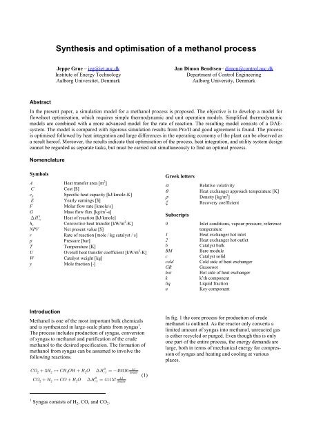
In fig. 1 the core <strong>process</strong> for production <strong>of</strong> crude<br />
<strong>methanol</strong> is outlined. As the reactor only converts a<br />
limited amount <strong>of</strong> syngas into <strong>methanol</strong>, unreacted gas<br />
is either recycled or purged. Even though this is only<br />
one part <strong>of</strong> the entire <strong>process</strong>, the energy dem<strong>and</strong>s are<br />
large, both in terms <strong>of</strong> mechanical energy for compression<br />
<strong>of</strong> syngas <strong>and</strong> heating <strong>and</strong> cooling at various<br />
places.<br />
CO + 3H ↔ CH OH + H O ∆ H = −49316<br />
2 2 3 2<br />
2 2 2<br />
0<br />
rx<br />
0<br />
rx<br />
CO + H ↔ CO + H O ∆ H = 41157<br />
kJ<br />
kmole<br />
kJ<br />
kmole<br />
(1)<br />
1 Syngas consists <strong>of</strong> H 2 , CO, <strong>and</strong> CO 2 .
fig. 1 Conceptual flowsheet for production <strong>of</strong> crude <strong>methanol</strong> from syngas.<br />
Optimisation <strong>of</strong> the <strong>process</strong> design is essential to obtain<br />
an economically feasible <strong>and</strong> competitive <strong>process</strong>. It is<br />
important to observe that in typical applications 80% <strong>of</strong><br />
the capital cost will be fixed very early in the project in<br />
the conceptual design (Biegler et al. 97). Therefore,<br />
changes in the subsequent phases will only be able to<br />
save a maximum <strong>of</strong> 20% <strong>of</strong> the total capital cost.<br />
The objective <strong>of</strong> this paper is to develop a model for a<br />
<strong>methanol</strong> <strong>process</strong> to be used, for flowsheet <strong>optimisation</strong><br />
during the conceptual design phase. The model<br />
must be simple enough for flowsheet <strong>optimisation</strong>,<br />
while still capturing the correct behaviour <strong>of</strong> the unit<br />
operations. On the other h<strong>and</strong>, detailed models are not<br />
necessary during conceptual design, as they <strong>of</strong>te requires<br />
more data than what is available early in the<br />
project. The flowsheet <strong>optimisation</strong> is implemented in<br />
GAMS (Brooke et al. 98) <strong>and</strong> in order to evaluate the<br />
models they will be compared with commonly accepted<br />
rigorous models found in Pro/II by (Invensys<br />
03).<br />
Modelling<br />
The model <strong>of</strong> the system includes a thermodynamic<br />
model <strong>of</strong> the chemical components, models <strong>of</strong> the individual<br />
unit operations <strong>and</strong> capital cost estimation.<br />
Since <strong>methanol</strong> plants are very large <strong>and</strong> operates continuously<br />
for more than 8000 hours per year, it is<br />
reasonable to use steady-state models for the flowsheet.<br />
(Biegler et al. 97). All together this is a simple thermodynamic<br />
model, requiring only few equations.<br />
Reactor model<br />
The reactor is modelled as a packed-bed-reactor (PBR),<br />
where the syngas flows through a catalyst bed. For this<br />
study it is assumed that the reactor operates adiabatically.<br />
A homogenous model is used, even though it is a<br />
simplified approach; we consider it adequate for the<br />
purpose <strong>of</strong> conceptual design. The reaction rates for<br />
<strong>methanol</strong> are quite complex however especially since a<br />
wide range <strong>of</strong> operating conditions must be covered in<br />
order to avoid constraints on the <strong>optimisation</strong>. (V<strong>and</strong>en<br />
Bussche <strong>and</strong> Froment 96) have proposed a rate expression<br />
that covers a range for 180°C
The energy equation for an adiabatic PBR with q reactions<br />
<strong>and</strong> m species can be formulated as:<br />
dT<br />
dW<br />
=<br />
q<br />
∑( −rij<br />
) ⎡−∆HRXij<br />
( T)<br />
⎤<br />
⎢<br />
⎥<br />
i=<br />
1<br />
m<br />
⎣<br />
∑<br />
j = 1<br />
Fc<br />
j p,<br />
j<br />
Conservation <strong>of</strong> momentum in a packed bed is modelled<br />
by the Ergun equation, (Fogler 99). Assuming an<br />
average density throughout the reactor, the expression<br />
can be reformulated into an algebraic equation.<br />
1<br />
2<br />
( )<br />
2 2 in out 2 tin , tout ,<br />
out in 0<br />
total<br />
2 2T0 2Ft<br />
0<br />
⎦<br />
(4)<br />
α T + T F + F<br />
p − p = − p W (5)<br />
It must be noted that the assumption <strong>of</strong> constant density<br />
does not hold in reality, but the simplified equation will<br />
provide an estimate for the pressure drop through the<br />
reactor.<br />
Flash calculations<br />
In the flash calculation the simplified model proposed<br />
by (Biegler et al. 97) is used. A keycomponent is selected<br />
from which the recovery <strong>of</strong> the non-key components<br />
can be calculated as:<br />
α<br />
ξ<br />
k<br />
kn , n<br />
0<br />
k<br />
= ; αk,<br />
n<br />
=<br />
n<br />
1+ −1<br />
ξ<br />
p<br />
n<br />
0<br />
ξ<br />
( αkn<br />
, )<br />
p<br />
(6)<br />
In addition, the bubble-point equation must be fulfilled:<br />
p = ∑ y p<br />
(7)<br />
i<br />
i<br />
liq, i 0<br />
The flash is considered adiabatic, <strong>and</strong> hence the outlet<br />
temperature is equivalent to the inlet. The pressure<br />
drop through the flash vessel is assumed zero.<br />
Heat exchangers<br />
The heat transfer in the heat exchangers are normally<br />
based on the logarithmic mean temperature difference,<br />
but this method fails if the flow capacity rates for the<br />
two sides <strong>of</strong> the heat exchanger are identical, <strong>and</strong> besides<br />
the method is numerically unstable. Therefore,<br />
the following approximation proposed by (Paterson 84)<br />
is used.<br />
2 1<br />
Q<br />
= UA∆Tlm<br />
≈ UA( 3<br />
θθ<br />
1 2+ 6( θ1+<br />
θ2)<br />
)<br />
1 1 1<br />
≈ +<br />
U h h<br />
c, hot c,<br />
cold<br />
The convective heat transfer coefficients are estimated<br />
from (Peters et al. 03); while only an estimate, this<br />
eliminates the need for a detailed heat exchanger design.<br />
(8)<br />
Sizing <strong>and</strong> cost estimation<br />
Capital costs are approximated by the methods described<br />
in (Turton et al. 98). The cost equations cover a<br />
very large range, which makes them highly non-linear.<br />
Therefore, a set <strong>of</strong> equations have been derived to<br />
cover the specific area <strong>of</strong> application considered in this<br />
paper, see the appendix. The grassroot cost 2 <strong>of</strong> a plant<br />
is<br />
Units<br />
Units<br />
0<br />
GR<br />
= 1.18<br />
BM , i<br />
+ 0.35<br />
BM , i<br />
i= 1 i=<br />
1<br />
∑ ∑ (9)<br />
C C C<br />
0<br />
The bare module cost at base conditions ( C<br />
BM<br />
) are<br />
0<br />
calculated as the bare module cost ( C<br />
CM<br />
) at ambient<br />
pressure <strong>and</strong> carbon steel construction. The sizing <strong>of</strong><br />
the equipment are carried out along the following<br />
guidelines<br />
• Pressure vessels are assumed to have a length<br />
to diameter ratio <strong>of</strong> four.<br />
• The volume <strong>of</strong> the flash vessel is twice the<br />
volume needed for a liquid hold up time <strong>of</strong> 5<br />
minutes.<br />
• All components are constructed using<br />
stainless steel.<br />
Finally, it is chosen to use the Net Present Value as the<br />
objective function for the <strong>optimisation</strong> problem<br />
10<br />
En<br />
NPV = − CGR<br />
+ ∑ n<br />
(10)<br />
( + i)<br />
n=<br />
1 1<br />
Solution procedure<br />
Given the models outlined in the previous section, it is<br />
possible to optimise the flowsheet. When the flow<br />
sheet is optimised, <strong>and</strong> the temperature levels are determined<br />
heat integration is carried out. This is in line<br />
with the hierarchical design method proposed by<br />
(Douglas 88), where the most important part <strong>of</strong> the<br />
<strong>process</strong> is designed first.<br />
All the unit operation models along with thermodynamic<br />
models <strong>and</strong> kinetic models have been implemented<br />
into a database. Given a flowsheet structure<br />
provided through the user interface a GAMS-datafile is<br />
generated <strong>and</strong> sent to GAMS. The problem is solved in<br />
GAMS <strong>and</strong> the results returned to the user-interface.<br />
Subsequently the results can be used as input to the<br />
Pro/II simulation program for a more rigorous simulation.<br />
Solution <strong>of</strong> ODEs<br />
The reactor model results in a number <strong>of</strong> ODEs that<br />
need to be solved, <strong>and</strong> since they cannot be solved<br />
2 Grassroot cost is a common term in chemical engineering<br />
referring to a completely new facility, i.e. the<br />
construction is started on a grass field.
analytically, a numerical method must be applied. Several<br />
methods are available, e.g. the well-known Runge-<br />
Kutta method. However, for <strong>optimisation</strong> we need the<br />
problem transformed into a number <strong>of</strong> algebraic equations,<br />
<strong>and</strong> for this purpose the method <strong>of</strong> orthogonal<br />
collocation points on finite elements (OCFE) have been<br />
successfully applied in a number <strong>of</strong> studies, e.g.<br />
(Biegler et al. 02). In fig. 2 two different meshes (3 <strong>and</strong><br />
5 elements, both with 2 collocation points) are compared<br />
to the solution obtained by a st<strong>and</strong>ard ODEsolver.<br />
Three elements are too few, with large deviations<br />
from the st<strong>and</strong>ard ODE-solver. Five elements<br />
provide a far better solution; there still are some discrepancies,<br />
but nevertheless the outlet conditions match<br />
very well. In relation to the rest <strong>of</strong> the system, the output<br />
from the reactor is <strong>of</strong> primary interest rather than<br />
the internal states, <strong>and</strong> therefore five elements are considered<br />
sufficient for this purpose.<br />
0.14<br />
0.12<br />
ODE<br />
OCFE<br />
T=200 C<br />
0.14<br />
0.12<br />
ODE<br />
OCFE<br />
T=200 C<br />
0.1<br />
T=220 C<br />
0.1<br />
T=220 C<br />
Methanol flow [kmole/s]<br />
0.08<br />
0.06<br />
0.04<br />
T=240 C<br />
T=190 C<br />
T=280 C<br />
Methanol flow [kmole/s]<br />
0.08<br />
0.06<br />
0.04<br />
T=240 C<br />
T=190 C<br />
T=280 C<br />
0.02<br />
0.02<br />
0<br />
0 0.1 0.2 0.3 0.4 0.5 0.6 0.7 0.8 0.9 1<br />
Normalised length [-]<br />
0<br />
0 0.1 0.2 0.3 0.4 0.5 0.6 0.7 0.8 0.9 1<br />
Normalised length [-]<br />
fig. 2 Simulation <strong>of</strong> <strong>methanol</strong> formation with different reactor inlet temperatures. To the left three elements have been used<br />
<strong>and</strong> to the right five elements have been used. The dotted line are the solution by a traditional ODE-solver.<br />
Heat integration<br />
The synthesis <strong>of</strong> the heat exchanger network is based<br />
on the method described by (Yee et al. 90), where a<br />
super structure for the heat exchanger network is proposed.<br />
The cost estimation method used in this paper is<br />
slightly different however, so the method has been<br />
changed to fit into the present work.<br />
Results<br />
The <strong>process</strong> from the <strong>optimisation</strong> can briefly be summarised<br />
as:<br />
• Reactor inlet conditions: T=473 K, p=45.5 bar<br />
• Flash conditions: T=321 K, p = 44.7 bar<br />
• Purge rate: 5%<br />
0.05<br />
0.045<br />
ODE<br />
OCFE<br />
Concentration pr<strong>of</strong>iles<br />
y CH3OH<br />
530<br />
ODE<br />
OCFE<br />
Temperature pr<strong>of</strong>iles<br />
0.04<br />
520<br />
0.035<br />
y CO<br />
510<br />
0.03<br />
y H2O<br />
0.025<br />
500<br />
0.02<br />
0.015<br />
490<br />
0.01<br />
y CO2<br />
480<br />
0.005<br />
0<br />
0 0.1 0.2 0.3 0.4 0.5 0.6 0.7 0.8 0.9 1<br />
470<br />
0 0.1 0.2 0.3 0.4 0.5 0.6 0.7 0.8 0.9 1<br />
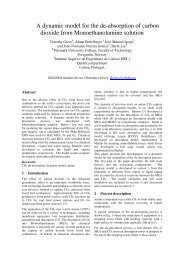
fig. 3 Comparison <strong>of</strong> reactor model in GAMS <strong>and</strong> a rigorous model. The GAMS model has calculated the results at the collocation<br />
points (marked with crosshairs), while the rigorous model is represented by the continuous curves.
Comparison with rigorous <strong>process</strong> model<br />
The <strong>optimisation</strong> has been carried out with simplified<br />
models, <strong>and</strong> for verification the result is compared with<br />
rigorous models from Pro/II (Invensys 03), see fig 3. It<br />
is obvious that the finite element mesh is too crude to<br />
capture the exact behaviour <strong>of</strong> the reactor, <strong>and</strong> clearly<br />
numerical instabilities are observed in the last part <strong>of</strong><br />
the reactor. Still the outlet conditions actually match<br />
quite well, which is regarded to be very important in<br />
relation to the rest <strong>of</strong> the flowsheet.<br />
fig. 4 Comparison <strong>of</strong> the utility dem<strong>and</strong> calculated by<br />
Pro/II <strong>and</strong> the simplified models<br />
The utility dem<strong>and</strong> calculated by the simplified models<br />
agrees quite well with the rigorous models. It is considered<br />
adequate for flowsheet <strong>optimisation</strong>. The flash<br />
model shows some deviations regarding the fraction <strong>of</strong><br />
light components in the liquid fraction. Still the level <strong>of</strong><br />
the major liquid components (<strong>methanol</strong> <strong>and</strong> water)<br />
agrees very well, implying that the deviations only<br />
have very limited impact on the result.<br />
fig. 5 Comparison <strong>of</strong> the flash calculation by Pro/II<br />
<strong>and</strong> the simplified calculations. Note the use <strong>of</strong> a<br />
logarithmic scale.<br />
Discussion <strong>of</strong> <strong>optimisation</strong> results<br />
Considering the yearly operating costs, it is very interesting<br />
to notice that steam <strong>and</strong> electricity accounts for<br />
more than 90% <strong>of</strong> total, fig. 6. On the other h<strong>and</strong>, the<br />
feed <strong>and</strong> cold utility cost is almost negligible in this<br />
context. The consequence is that the hot utility <strong>and</strong><br />
electricity has major influence on the overall economy<br />
<strong>of</strong> the plant, <strong>and</strong> thereby on the <strong>optimisation</strong> problem.<br />
If heat integration is applied to the <strong>process</strong> the need for<br />
hot utility can be eliminated, see fig. 6 <strong>and</strong> fig. 7.<br />
fig. 6 Annual operating costs both with <strong>and</strong> without<br />
heat integration<br />
fig. 7 Heat exchanger network for heat integrated<br />
plant. Please note that the condenser is split into a<br />
de-superheating section <strong>and</strong> a condensing section<br />
As the hot utility can be eliminated, it will have a major<br />
impact on the <strong>optimisation</strong> <strong>of</strong> the core <strong>process</strong>, as<br />
the annual operating cost would be significantly reduced.<br />
It is important to recognise the high impact<br />
from the operating costs, especially hot utility <strong>and</strong><br />
electricity, making it necessary for the <strong>optimisation</strong> <strong>of</strong><br />
heat exchanger network <strong>and</strong> utility system to be included<br />
at a very early stage. Otherwise, there is a significant<br />
risk that the overall solution ends up being<br />
suboptimal. In a future paper a more integrated approach<br />
for the design will be set forth, but so far it has<br />
only been recognised that the problem exists.
Conclusion<br />
Paterson, W. R. (84) A replacement for the logarithmic<br />
mean Chemical Engineering Science, 39(11), 1635-<br />
In the present paper, a simulation model for a <strong>methanol</strong><br />
1636<br />
<strong>process</strong> has been proposed, which can be used for<br />
Peters, M. S., Timmerhaus, K. D., <strong>and</strong> West, R. E. (03)<br />
flowsheet <strong>optimisation</strong> purposes. The model combines<br />
Plant Design <strong>and</strong> Economics for Chemical Engineers<br />
5th.ed., McGraw-Hill, ISBN: 0-07-119872-5<br />
simplified thermodynamic models, with a more advanced<br />
model for the rate <strong>of</strong> reaction. The resulting<br />
Turton, R. <strong>and</strong> others (98) Analysis, synthesis, <strong>and</strong><br />
model consists <strong>of</strong> a DAE-system discretising the ODEs<br />
design <strong>of</strong> chemical <strong>process</strong>es 1.ed., Prentice Hall,<br />
with orthogonal collocation points on finite elements<br />
ISBN: 0-13-570565-7<br />
an algebraic equation system is obtained. The model at<br />
V<strong>and</strong>en Bussche, K. M. <strong>and</strong> Froment, G. F. (96) A<br />
the optimum point is compared with rigorous models<br />
steady-state kinetic model for <strong>methanol</strong> synthesis<br />
from Pro/II <strong>and</strong> there is a good agreement between the<br />
<strong>and</strong> the water gas shift reaction on a commercial<br />
results.<br />
Cu/ZnO/Al2O3 catalyst Journal <strong>of</strong> Catalysis, 161,<br />
A closer look at the <strong>optimisation</strong> results shows that<br />
there is a very large potential for energy <strong>and</strong> economic<br />
saving, which will have a major influence on the plants<br />
economy. It must be concluded that a sequential design<br />
procedure, in which the heat integration <strong>and</strong> utility<br />
1-10<br />
Yee, T. F., Grossmann, I. E., <strong>and</strong> Kravanja, Z. (90)<br />
Simultaneous optimization models for heat integration<br />
- II. Heat exchanger network synthesis Computers<br />
& Chemical Engineering, 14(10), 1165-1184<br />
system design is done after <strong>optimisation</strong> <strong>of</strong> the <strong>process</strong><br />
probably leads to sub optimal solutions. In a future<br />
Appendix<br />
paper, a comprehensive design method for simulataneous<br />
<strong>optimisation</strong> <strong>of</strong> <strong>process</strong>, heat <strong>and</strong> utility supply will<br />
be presented.<br />
Reference List<br />
Biegler, L. T., Cervantes, A. M., <strong>and</strong> Wächter, A. (02)<br />
Advances in simultaneous strategies for dynamic<br />
Kinetic data<br />
The constants for the rate equations are given in table<br />
1.<br />
table 1 Parameter values in the kinetic model.<br />
T is given in [K] <strong>and</strong> R g is 8.315 kJ/kmole-K<br />
<strong>process</strong> optimization Chemical Engineering Science,<br />
57, 575-593<br />
k = A exp(B / (R g T)) A B<br />
k<br />
Biegler, L. T., Grossmann, I. E., <strong>and</strong> Westerberg, A.<br />
a [bar -0,5 ] 0.499 17,197<br />
W. (97) Systematic methods <strong>of</strong> chemical <strong>process</strong><br />
k b [bar -1 ] 6.62e-11 124,119<br />
design 1.ed., Prentice Hall, ISBN: 0-13-492422-3<br />
k c [-] 3,453.38 0<br />
Brooke, A., Kendrick, D., Meeraus, A., <strong>and</strong> Raman, R. k d [mole / (kg-s-bar 2 )] 1.07 36,696<br />
(98) GAMS © GAMS Development Corporation<br />
k<br />
www.gams.com<br />
e [mole / (kg-s-bar)] 1.22e10 -94,765<br />
Douglas, J. M. (88) Conceptual design <strong>of</strong> chemical<br />
kd<br />
/ K<br />
1<br />
[mole / (kg-s)] 4.182e10 -22,005<br />
<strong>process</strong>es 1.ed., McGraw-Hill, ISBN: 0-07017762-<br />
eq<br />
kK e 3 [mole / (kg-s-bar)] 1.142e8 -55,078<br />
7<br />
Fogler, H. S. (99) Elements <strong>of</strong> Chemical Reaction<br />
Cost estimation<br />
Engineering 3.ed., Prentice-Hall, ISBN:<br />
0139737855<br />
The cost estimation functions used in this article are<br />
Invensys (03) Pro/II © Invensys SimSci-Esscor<br />
summarised in table 2 <strong>and</strong> table 3.<br />
www.simsci.com<br />
table 2 Cost estimation functions for major <strong>process</strong> equipment<br />
Equipment Purchased cost [$] Pressure correction [-] Bare module cost [$] Range<br />
Pressure vessel 3 0.5457<br />
0<br />
C = 3254.9V<br />
F 0.0369p<br />
1.3644 C = C 1.62 + 1.47F F 0.1-200 m 3<br />
p<br />
Compressors 4 0.9542<br />
C = 987.42W<br />
-<br />
Heat exchangers<br />
p<br />
Cp<br />
= 719.15A<br />
0.6518<br />
p<br />
Fp<br />
= +<br />
BM p ( M p )<br />
C<br />
0<br />
BM FMCp<br />
0.0988<br />
0<br />
= 0.7884p<br />
CBM Cp ( 1.8 1.5FM Fp<br />
)<br />
table 3 Material factors (F M )<br />
Equipment Carbon steel Stainless steel Nickel Alloy<br />
Pressure vessel 1.0 4.0 9.8<br />
Compressors 2.5 6.3 13.0<br />
Heat exchangers 1.0 3.0 3.8<br />
= 100-8000 kW<br />
= + 50-900 m 2<br />
3 Only applicable for a length:diameter ratio <strong>of</strong> 4<br />
4 Only applicable for centrifugal compressors