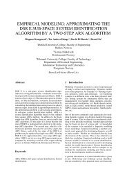
An Overview of the Marine Systems Simulator (MSS): A Simulink ...

An Overview of the Marine Systems Simulator (MSS):
A Simulink R Toolbox for Marine Control Systems
T. Perez ∗⋆ , Ø.N. Smogeli †⋆ , T.I. Fossen ‡⋆ , and A.J. Sørensen †⋆
⋆ Centre for Ships and Ocean Structures—CeSOS
† Department of Marine Technology
‡ Department of Engineering Cybernetics
Norwegian University of Science and Technology—NTNU
NO-7491 Trondheim, NORWAY
Abstract
The Marine Systems Simulator (MSS) is an environment
which provides the necessary resources for
rapid implementation of mathematical models of marine
systems with focus on control system design.
The simulator targets models—and provides examples
ready to simulate—of different floating structures
and its systems performing various operations.
The platform adopted for the development of MSS
is Matlab/Simulink R . This allows a modular simulator
structure, and the possibility of distributed development.
Openness and modularity of software components
have been the prioritized design principles,
which enables a systematic reuse of knowledge and
results in efficient tools for research and education.
This paper provides an overview of the structure of the
MSS, its features, current accessability, and plans for
future development.
1 Introduction
The Marine Systems Simulator (MSS) is a Simulink R -
based environment that provides the necessary resources
for rapid implementation of mathematical
models of marine systems with focus on control system
design. Its development started at the Norwegian
university of Science and Technology (NTNU) and is
ongoing with the help of other groups.
Since the early 1990s, significant resources have been
allocated to the area of marine control systems at
NTNU. This has resulted in numerous models and
simulation tools developed and used by students and
∗ Corresponding author; Email:
tristan.perez@ntnu.no
researchers. MSS provides an integration of these separated
efforts and allows researchers and students outside
NTNU to use it and contribute to further developments.
The name MSS was decided in 2004 to describe
the merge of three toolboxes oriented to marine
system simulation: Marine GNC Toolboox, MCSim,
and DCMV.
The Marine GNC toolbox was originally developed
by T.I. Fossen and his students as a supporting tool
for his courses on guidance and control of marine
vehicles and his book (Fossen, 2002). This toolbox
has provided the core library for MSS. The MCSim
was a complete simulator mostly oriented toward dynamic
positioning (DP) marine operations. This toolbox
was initiated by A.J. Sørensen and developed
by Ø.N. Smogeli and MSc students at the Department
of Marine Tehcnology at NTNU, as a source of
common knowledge for new MSc and PhD students,
see Sørensen et al. (2003). MCSim incorporated sophisticated
models at all levels (plant and actuator),
which have now been refactored into two libraries of
MSS. The DCMV toolbox was developed by Perez
and Blanke (2003) and was a reduced set of Simulink
blocks oriented to autopilot design. MSS incorporates
a small set of blocks from DCMV and functions related
to wave spectra, and actuators.
Since the merge leading to MSS, there has been a continuous
effort at NTNU by the authors and others to
provide a user friendly environment which can target
different simulation scenarios with the required level
of complexity for different marine operations—some
goals have been successfully achieved, but the work is
ongoing. The rest of the paper describes the current
structure of the MSS, its features, accessability, and
plans for future development.

User
Education
Research Industry
Model complexity
Research Academic
Simulation
Scenario
Process plant models
Control plant models
Low level (actuator) models
Implementation
Felxibility
Elementary components
Full systems
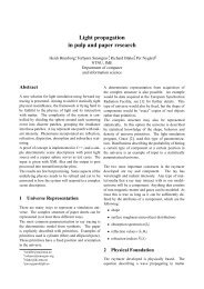
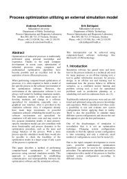
Figure 1: Simulation scenario space
2 MSS scope
The scope of a simulator is defined in terms of the different
simulation scenarios it can handle. These different
scenarios can be further specified according to the
following elements:
• Model complexity,
• Implementation flexibility,
• User proficiency.
Figure 1 illustrates this concept by making an analogy
to our familiar three-dimensional space.
The model complexity is determined by the purpose of
the model and its simulation. In mathematical modeling,
there is a fundamental trade-off between models
of great complexity, which yield a highly accurate description
of many aspects of real systems and simplified
models, which capture the fundamental aspects of
the system and are mathematical tractable for analysis
(Naylor and Sell, 1982). Within the control literature
complex models (process plant models) are used
to test control strategies and benchmark the more simple
models (control plant models) used for the design
of control strategies and analysis (e.g., robustness, stability,
fundamental limitations) (Goodwin et al., 2001;
Sørensen, 2005b; Sørensen, 2005a; Perez, 2005).
A simulator for marine systems (ships, offshore structured,
underwater vehicles, fisheries, etc.) needs to
account further for the variability of the models according
to the particular operation performed by the
vessel, state of the sea, and speed. Changes in these
system attributes result in changes in the response of
the marine system, response of actuators, and control
objectives, which in turn may lead to the need of different
types of models. For example, consider the case
of dynamic positioning (DP) of an offshore vessel. In
calm to medium seas, the main control objective of the
DP system could be to regulate the position (North,
East and heading) by rejecting slowly varying disturbances
due to mean wave forces, current and wind.
As the severity of the sea state increases, the oscillatory
motion induced by the waves often needs to be
included as a disturbance and the reduction of pitchand
roll-induced wave oscillatory motion can be incorporated
as additional control objectives. This demands
changes in the models (number of DOF, and
disturbance models) used by the observers and control
system.
The implementation flexibility of a simulator describes
whether existing models and simulation scenarios can
be easily adapted to implement new types of systems
using the allocated resources. This is a particularly
challenging aspect of marine system simulators due
to the diversity of ships and offshore structures and
the operations they perform. Therefore, openness and
modularity of software components have to be prioritized
as design principles for systematic reuse of
knowledge. In the case of MSS, Simulink R has been
adopted as a development platform because of the following
reasons:
• Simulink R offers the necessary modularity and
ease of implementation required for a flexible
simulator.
• Matlab R and Simulink R have become a tool
widely used in education and research; this adds
to the flexibility of MSS, because many students
and scientists have access to this development
platform.
• Matlab R has the great advantage that the many
low-level issues have been addressed: numerical
integration routines, plotting tools, data exchange
and exporting facilities.
• The real-time workshop facilities of
Matlab R /Simulink R provides a way of rapidly
generating prototype controllers based on
Simulink diagrams that run in real time on
stand-alone computer systems for tests on scale
models or full scale systems. This also offers
the possibility of implementing hardware-in-theloop
simulations. This is particularly important
for us, at NTNU, because students can easily
implement their controllers in the scale models
at the Marine Cybernetics Laboratory—see
http://www.itk.ntnu.no/marinkyb/MCLab/

o n
x n North
y n East
z n Down
o h
z h
x h
y h
o b
r
Heave
z b ,w
p
Surge
x b ,u
q
Sway
y b ,v
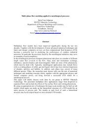
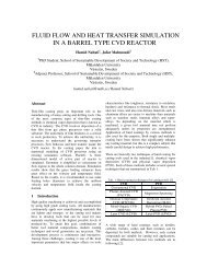
Figure 2: Notation and sign conventions for ship motion
description.
With regards to users, MSS offers different options.
MSS originally evolved as a way of increasing accessibility
and reuse of knowledge for students and
researchers at NTNU. Different components of what
now is MSS have been used in education and research
for several years and it incorporates several demos of
complete systems in particular operations. However,
due to its modularity and organisation, MSS offers a
core library of elementary blocks and functions which
can be combined to generate new systems to cover research
needs in both industry and academia.
3 Mathematical models in MSS
To understand the software organization of MSS, let us
briefly review the main components of models a marine
system. At the same time, we will introduce the
main conventions adopted in MSS.
3.1 Reference frames and magnitudes
To describe the general motion of a marine system,
we need to consider three coordinates to define translations
and three coordinates to define the orientation
(6DOF). These coordinates are defined using two
types of reference frames: inertial frames and bodyfixed
frames. Figure 2 shows the different reference
frames adopted in MSS, which are further specified
below (Fossen, 2002; Sørensen, 2005b; Sørensen,
2005a; Perez, 2005):
• North-east-down frame (n-frame). The n-
frame (o n ,x n ,y n ,z n ) is fixed to the Earth. The
positive x n -axis points towards the North, the positive
y n -axis towards the East, and the positive z n -
axis towards the centre of the Earth. The origin,
o n , is located on mean water free-surface at an appropriate
location. This frame is considered inertial.
• Body-fixed frame (b-frame; forwardstarboard-down).
The b-frame (o b ,x b ,y b ,z b )
is fixed to the hull. The positive x b -axis points
towards the bow, the positive y b -axis points
towards starboard and the positive z b -axis points
downwards. For marine vehicles, the axes of this
frame are chosen to coincide with the principal
axes of inertia; this determines the position of the
origin of the frame, o b .
• Hydrodynamic frame (h-frame; forwardstarboard-down).
The h-frame (o h ,x h ,y h ,z h ) is
not fixed to the hull; it moves at the average
speed of the vessel following its path. The x h -
y h plane coincides with the mean-water free surface.
The positive x h -axis points forward and it
is aligned with the low-frequency heading angle
ψ 1 . The positive y h -axis points towards starboard,
and the positive z h -axis points downwards.
The origin o h is determined such that the z h -axis
passes through the time-average position of the
centre of gravity. This frame is usually considered
when the vessel travels at a constant average
speed (which also includes the case of zero
speed); and therefore, the wave-induced motion
makes the vessel oscillate with respect to the h-
frame. This frame is considered inertial.
Each of these frames has a specific use. For example,
the n-frame is used to define the position and orientation
of the vessel as well as the current and wind
direction. The linear and angular velocity and acceleration
measurements taken on board are referred to the
b-frame, which is also used to formulate the equations
of motion. The h-frame is used in hydrodynamics to
compute the forces and motion due to the interaction
between the hull and the waves in particular scenarios.
These data are generally used for preliminary ship design
(Couser, 2000); and therefore, it can also be used
to obtain models. The h-frame is also used to define
local wave elevation and to calculate indices related to
performance of the crew or comfort of passengers—
see Perez (2005).
1 The angle ¯ψ is obtained by filtering out the 1st-order waveinduced
motion (oscillatory motion), and keeping the low frequency
motion, which can be either equilibrium or slowly-varying.
Hence, ¯ψ is constant for a ship sailing in a straight-line path.

The north-east-down position of a ship is defined by
the coordinates of the origin of the b-frame, o b , relative
to the n-frame:
r n o b
[ n, e, d ] T
.
The attitude of a ship is defined by the orientation of
the b-frame relative to the n-frame. This is given by
the vector of Euler angles,
Θ nb [ φ, θ, ψ ] T
, (1)
which take the n-frame into the orientation of the b-
frame. Following the notation of Fossen (1994; 2002),
the generalised position vector (or position-orientation
vector) is defined as:
[ ] r
n
η ob
= [n,e,d,φ,θ,ψ] T . (2)
Θ nb
The linear and angular velocities of the ship are more
conveniently expressed in the b-frame. The generalised
velocity vector (or linear-angular velocity vector)
given in the b-frame is defined as:
[ ] v
b
ν ob
ω b = [u,v,w, p,q,r] T , (3)
nb
where
• v b o b
= [u,v,w] T is the linear velocity of the point
o b expressed in the b-frame—see Figure 2.
• ω b nb = [p,q,r]T is the angular velocity of the b-
frame with respect to the n-frame expressed in the
b-frame.
Table 1 summarizes the adopted notation.
3.2 Equations of motion
Using the notation of the previous section, the general
form of the equations of motion of a marine system
can be written in a vector form as
M˙ν+C(ν,ν r )+D(ν r ,µ)+g(η) = τ env + τ ctrl , (4)
˙µ= A m µ+ B m ν r , (5)
˙η = J n b (Θ nb)ν, (6)
where M = MRB b + Mb A
is the total mass matrix (rigid
body + constant added mass) with all the moments and
products of inertia taken with respect to the origin of
the b-frame. The velocity ν r is the velocity relative to
the current, i.e., ν r = ν − ν c , where ν c is the velocity
of the current expressed in the b-frame. The function
Mag. Name Frame
n North position n-frame
e East position n-frame
d Down position n-frame
φ Roll ang. Euler ang.
θ Pitch ang. Euler ang.
ψ Heading (yaw) ang. Euler ang.
u Surge velocity b-frame
v Sway velocity b-frame
w Heave velocity b-frame
p Roll rate b-frame
q Pitch rate b-frame
r Yaw rate b-frame
Table 1: Adopted nomenclature for the description of
ship motion, and reference frames in which the different
magnitudes are defined.
C(ν,ν r ) = C b RB (ν)ν + Cb A (ν r)ν r gives the forces due
to fictitious accelerations (Coriollis and Centripetal)
that appear when expressing the equations of motion
in a non-inertial frame. These forces have two components:
one proportional to the rigid body mass and
another proportional to the added mass—see Fossen
(2002) for details. The terms D(ν r ,µ) are the damping
terms, which can be separated into different components:
D(ν r ,µ) = D b p1ν r + D b p2µ+ D b Visc(ν r ), (7)
where the first two terms are the linear potential damping
due to the energy carried away by the waves generated
by the ship, and the last term accounts for viscous
effects. The variables µ in the (5) account for the fluid
memory effects associated with the radiation problem
(waves generated by the ship). This equation together
with the first two terms in (7) is a state-space representation
of the convolution integral in the Cummins
Equation—see Fossen (2005) or Perez (2005) for further
details.
The terms g(η) in (4) are the so-called restoring forces
due to gravity and buoyancy, which tend to restore the
up-right equilibrium position of the ship. These forces
also incorporate the effect of mooring systems if any.
As indicated in (4), these are function of the position
and orientation of the system. Equation (6) is the kinematic
transformation between the vector of linear and
angular velocities in the b-frame and the time derivatives
of the position and Euler angles.
On the right-hand side of (4) we have the environmental
excitation forces and the control forces. The envi-

onmental excitation forces are separated into wave,
wind and current loads. The wave forces are separated
into oscillatory or 1st-order wave forces (Froude-
Krilov and diffraction) and the 2nd-order wave loads
(mean-wave drift and slowly varying non-linear effects).
The current is accounted for in the model as
an offset velocity which affects the damping forces as
indicated in (7) and (5).
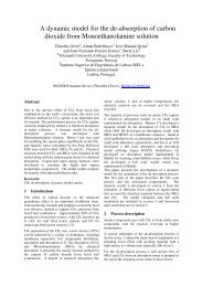
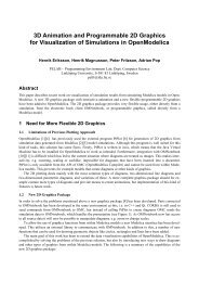
The control forces are those generated by the different
actuators: rudders, propellers, fins, thrusters, interceptors,
etc. Figure 3 shows a block diagram representation
of the main components of a marine system
as described by equations (4)-(6)—(Smogeli et
al., 2005). This figure also shows other components
often included in a ship motion control system—see
Fossen (2002), Sørensen (2005a) and Perez (2005) for
further details about modeling of marine vehicles.
Wind
Waves
External
loads
Environment
External
load models
Wind load
model
Wave drift
load model
Waves
Wind
Current
I
wind
Thrust
forces
W2
Froude-Krylov
and diffraction
forces W1
+
Vessel
dynamics
Thruster
dynamics
*
+
P
J* T
Thrust
forces
Motion
Motion
d
HS
Thrust
setpoints
Nonlinear
damping
Radiation
model
Rigid-body
equations of
motion
Restoring
forces
Sensors
Thrust
allocation
r
r
J*
+
Filtered &
reconstructed
signals
Desired
thrust
vector
Figure 3: Marine system components
v c
b
Current
Vessel
motion
Vessel
observer
Vessel
control
4 Software Characteristics and Organization
MSS is organized as a set of Simulink libraries, GUIs
and Matlab support functions:
• Marine GNC Toolbox,
• Add-in libraries:
– Marine Hydro
– Marine Propulsion
– Marine Systems
• Marine Visualization Toolbox (MVT),
• Matlab support functions,
The Marine GNC 2 Toolbox is the core component of
MSS, and most of the other components make use of it.
This core toolbox incorporates the SimulinkR library
marine gnc.mdl, and its associated support functions
(matlab functions). The add-in libraries incorporate
further functionality to MSS by adding more complex
components. At this stage, there are three add-ins
as indicated above. Some of these are still in progress,
and are available upon request—see Section 5 for software
availability. The Marine Visualization toolbox
has recently been incorporated to MSS, but this is an
independent toolbox. The integration with MSS results
in additional interfaces to generate the data used
by MVT.
In the following, we further describe each of the currently
available components.
4.1 Marine GNC Toolbox
The Marine GNC Toolbox is the core component
of MSS; it incorporates the simulink library
marine gnc.mdl, and its associated support functions
(matlab functions). This toolbox contains the
basic simulink blocks which allow implementing the
models described in Section 3 and also different vessel
models and examples ready to simulate.
After installing this toolbox, the entry Marine GNC
Toolbox should appear in the Simulink library brouser,
as shown in Figure 4.
The different blocks of the marine gnc.mdl library
are organized in the following seven modules (see Figure
4):
• Control: In this module there are blocks that
implement controllers for autopilots (PID controllers
tuned using the Nomoto model parameters)
and dynamic positioning (PID controllers
for set point regulation). Future controllers incorporate
hybrid controllers with motion damping
capabilities (stabilizers and rudder roll stabilization)
• Environment: In this module, there are blocks to
define the environmental conditions of each simulation
scenario: wind, wave and current. The
block waves provides all the Fourier components
(amplitudes, frequencies, and wave numbers) to
implement time series of a sea-surface elevation.
The user can choose among four different spectra
2 Guidance Navigation and Control

– A zig-zag test of a naval vessel.
– Turning manoeuvre of a naval vessel.
• Guidance: This module contains blocks to generate
reference trajectories for DP, path following
and autopilot systems. It contains reference
filters, a block for smooth trajectory generation
based on way points, and blocks to generate the
rudder command for ziz-zag, pull-out, and turning
tests.
Figure 4: Simulink library browser showing the Marine
GNC Toolbox after installation.
(ITTC, JONSWAP, Torsethaugen, and user specified).
The block allows spreading of the spectra
with respect to a mean direction and also regular
wave generations. To reduce the number of
fourier components used, the block incorporates
an energy-based method for eliminating components.
The block also incorporates options for
plotting the spectrum used in 3D, the Fourier
components, and a snapshot of the sea surface
generated by the chosen spectrum. This can be
used to check, before the simulations, the correct
state and degree of accuracy of the sea-state description.
• Examples: In the examples module, there are
seven single-block vessel models (CybershipIII,
Cargo, Semisub, supply vessel, tanker, naval vessel),
and ten demos ready to simulate:
– Four different autopilot designs using different
measurements and wave filters.
– Two DP examples.
– A thruster configuration demo for a supply
vessel.
– A wave point based guidance system.
• Models: This module contains all the necessary
blocks to implement the equations of motion (4)-
(6). This includes blocks for kinematic transformations
and equations of motion in 3, 4 and
6DOF, control surfaces (rudders and fins), environmental
load blocks (which combined with
the environment blocks provide the loads.) This
module also incorporate basic propulsion blocks
with open water characteristics of propellers, propeller
shaft dynamics, and propeller configuration
blocks for different DP vessels.
• Navigation: This module contains passivity- and
Kalman-based observers. Future version will incorporate
other filters, models of different sensors
(GPS,HPS,Microwave Systems,VRU,IMU,etc.)
• Utilities: This module includes blocks that perform
mathematical operations to related signals.
4.2 Marine Hydro add-in
One of the most difficult issues for anyone attempting
a control system design for a marine system is to obtain
an appropriate mathematical model. The Marine
Hydro add-in provides an interface with commonly
used hydrodynamic codes. These codes are widely
used by Naval architects during preliminary stages of
ship design, and provides most of the parameters necessary
to implement a model of a marine system that
could be used as an initial step in the control system
design process.
The Marine Hydro add-in provides matlab functions
that read the output files of different hydrodynamic
codes: ShipX-VERES (Fathi, 2004), SEA-
WAY (Jouernee and Adegeest, 2003), and WAMIT 3
(WAMIT, 2004), and generate a predefine data structure.
These codes use a geometrical definition of
the hull and its loading condition (distribution of
3 The WAMIT interface is still in progress, at the time of publication
of this paper.

mass) to calculate the following data: restoring coefficients,
added-mass and damping coefficients, exciting
forces transfer functions (force-RAOS), bodymotion
transfer functions (motion-RAOS), local hydrodynamic
pressure, mean-drift force and moment,
etc. All these data are commonly exported in ASCII
form in different files, and the Marine Hydro add-in
provides Matlab routines that extract all this information
and generate a data structure vessel for the particular
ship analyzed. Once vessel is generated, there
are different functions to plot data(added mass and
damping as a function of the frequency and RAOS),
functions to generate a state-space model for the fluid
memory effects, and a a special simulink model for
time domain simulations. The latter provides a seamless
interface for a rapid implementation of models of
marine vessels in three steps:
1. Load the ship data into a particular hydrodynamic
code (at this stage VERES and SEAWAY) , and
execute it.
2. Import the hydrodynamic data generated by the
codes into Matlab R using the functions of the
add-in. This defines the structure vessel in
matlab.
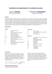
3. Use the Hydro add-in simulink model for timedomain
simulations in different sea states.
Hydrodynamic Codes
(VERES,OCTOPUS,WAMIT)
Hull geometry
Loading condition
Water depth
Mooring lines
Speed
Headings
Added Mass
Damping
Restoring forces/coefficients
MSS
Force RAO (Froude-Kriloff, diffraction)
Motion RAO
Wave-drift forces
MATLAB
Interface
Functions
Data
Structure
Sea State
Time-domain Simulations
Figure 5: Marine Hydro capabilities.
Figure 5 illustrates the process. Examples of use
of this add-in have been described in (Fossen and
Smogeli, 2004) and (Smogeli et al., 2005)
NOTE: The Marine Hydro add-in DOES NOT
provide licences and/or copies of the hydrodynamic
codes for which the interfaces have been developed.
The user should obtain appropriate licensed copies of
these codes.
4.3 Marine Propulsion add-in
The MSS Marine Propulsion Add-In targets simulation
and control design for propellers, thrusters, and
rudders. The current library consists of blocks for propeller
characteristics, various hydrodynamic calculations
and thrust loss models, motor models, sensors,
control systems, and a variety of other tools. In addition,
complete models compiled from the basic blocks
are included.
Five different models of the propeller hydrodynamics
have been implemented, producing the nominal (openwater)
propeller thrust and torque. Two model representations
for open and ducted fixed-pitch propellers
(FPP), one 4-quadrant and one 1-quadrant model, are
available, taking propeller shaft speed and propeller
advance velocity as input. Similarly, two model representations
for open and ducted controllable-pitch propellers
(CPP), one 4-quadrant and one 1-quadrant, are
available, taking propeller shaft speed, propeller advance
velocity, and propeller pitch as input. The
1-quadrant model is also suitable for CPP tunnel
thrusters. Finally, a cavitation number based model
for FPP tunnel thrusters is available, taking propeller
shaft speed and tunnel submergence as input. Note
that all models require the user to input some kind of
propeller characteristics, either from known propeller
series, from a propeller analysis program, or from experiments.
Thrust losses due to the presence of the hull in terms
of wake and thrust deduction is accounted for, as well
as loss effects due to variations in advance velocity,
cross-coupling drag for open and ducted propellers
due to transverse fluid velocity, speed loss for tunnel
thrusters due to vessel surge velocity, and ventilation
and in-and-out-of-water effects, including the Wagner
effect. The relative motion of the thruster with respect
to the water is calculated from vessel 6 DOF motion,
waves and current. Additional loss effects, e.g. the
Coanda effect and thruster-thruster interaction, are under
development.
Simplified models of the thruster motors, as well as azimuth
and pitch dynamics are available, including rate
saturation and physical limits. A propeller shaft model
is also present, including friction and shaft inertia.
Blocks for conventional shaft speed control, torque

control, power control, and combined power/torque
control are available. Sensor models including white
noise and quantizing are also available in order to give
realistic feedback signals.
A thruster dynamics module, compiled of the various
propeller characteristics, loss effects, and motor models
has been included in the library. This shows how
the basic building blocks can be used to build more
complex models. A closed-loop model, including sensors
and control systems, is also available. These modules
require extensive user input for use, and are intended
for in-house research on propulsion control.
4.4 Marine Systems add-in
The Marine Systems add-in is a simulink library with
complex system ready to simulate—which has not yet
been released. This library is to be used mostly for
education purposes as an aid to illustrate concepts in
class and by letting students experiment with what
they have learned instead of fighting the common (and
necessary) blunders they make while implementing
complex systems in Simulink. This library can also be
used for application of novel control and identification
techniques on benchmark examples.
4.5 Marine Visualization Toolbox (add-in)
The Marine Visualization Toolbox MVT add-in displays
data from simulations, experiments or measurements
of marine systems as 3D animations. The animations
may be viewed on-line or saved to file. This
toolbox was developed at the Department of Engineering
Cybernetics NTNU (Danielsen et al., 2004), and
is available independent of MSS, but integration with
MSS is ongoing.
MVT uses features of the Matlab Virtual Reality Toolbox,
which is an interface for viewing 3D models.
The resulting animations depict vessel moving and rotating
according to the time-varying input data. Figure
6 shows a snapshot of one of such animations for
scale vessel on a replenishment operation (Kyrkjebø
and Pettersen, 2003). The input data may represent a
maximum of six degrees of freedom (6 DOF) in terms
of the xyz-positions and Euler angles. With the current
version of MVT, these data need to be assembled
into a special strucutre by the user. However, work
is currently being done on a special simulink block
that takes the velocity and position vectors ν(t k ) and
η(t k ) and save the data into the special structure to be
then used by MVT. Any number of vessels may be
animated at the same time. The vessels are animated
Figure 6: Snapshot of an MVT animation based on
experiments of a scale vessel on a replenishment operation.
in a scene model (e.g. a coastline or a harbor) representing
the actual surroundings of the simulations, experiments
or full scale measurements. Both scene and
vessel models are implemented in the Virtual Reality
Modeling Language (VRML).
MVT includes two libraries of VRML files; vessel
models and scenes. Combinations of these are generated
to resemble specific scenarios with the desired
number and types of vessels located in the desired
surroundings. For further details see Danielsen et al.
(2004) and the links at the MSS web site (see next section).
5 Where to find it and Access Level
MSS is free, i.e., there is no fee for using MSS;
however, some of its components may be of restricted
distribution. Then only conditions for the use of any
of the MSS components is the acknowledgement of
the publication of any result obtained using MSS,
and reporting back any bugs and contributions. The
current version of MSS, and conditions for use can be
found at:
http://www.cesos.ntnu.no/mss/
In this web site there are also documentation,
instructions for installation, previously released
versions, links to related literature, and MSS technical
reports.

At this stage, there are two access levels:
• Free: This incorporates the Marine GNC Toolbox
and all its support functions.
• Free Restricted: As MSS is to be used for research,
as well as for education, some models
may be sensitive and kept either in-house or be
shared only by collaborators. Therefore, some elements
of MSS will be of restrictive distribution.
The hydro and propulsion add-ins are currently
restricted to collaborators, and can be made available
upon request.
6.3 Dialog window
The dialog window is generated by the mask, and allows
to enter parameters to the block. Figure 7 shows
an example.
6 Elementary Blocks and Guidelines
for Contributions
Simulink blocks are elementary constitutive parts of
the MSS simulink libraries, and are used to create
other more complex blocks or models or both. A
masked block serves to establish a boundary for modular
modeling approach. This boundary is set by specifying
the following attributes of the block:
• Block name,
• Inputs and outputs name,
• Mask information,
• Help information.
The rules followed in the development of MSS are indicated
next.
6.1 Color code
When users create a new block they should name it
and mask it. Under the mask, the following color code
is to be used for easy recognition of elementary blocks
functions:
• Green—input port
• Red—output port
• Grey—logic
• Yellow—others
6.2 Name and ports
The block name is the first indication of the task performed.
The Inputs and output labels indicate how to
interconnect the block with other existing blocks: they
share the same labels. Do not include units in the port
labels, and Do not use the drop shadow option of format.
Figure 7: Example of dialog window.
We recommend every block to be masked even when it
does not requre parameters; this helps modularity and
more importantly it provides access to the help of the
block. The following information should be incorporated
in the dialog window:
• Brief Description and Formulae (if short).
• Inputs and outputs description with units in SI
and positive convention.
• Parameter description (if short, if not this goes in
the help).
• Copyright (C) 200X, NTNU (if you would like
your contribution to be incorporated in MSS you
have to give the copyright to NTNU.)
• Authors Name.
NOTE: Incorporate SI units in the parameter window
but not in the block port labels.

6.4 Help window
The help window is called from the dialog window
of the block. The help provides further description of
block functionality. Due to the potential of multi-user
development, MSS will not incorporate a user manual,
and all the help should be included in the mask. The
reason for this is that updating documents and blocks
is twice the work and difficult to coordinate among
different developers. Therefore, developers provide
enough documentation in the mask.
The documentation of the block should be written in
HTM and the code pasted in the help window of the
mask. Alternatively, users can generate an HTM file
and call it from the mask using:
web([’file:///’which(’Help blockName.htm’)]);
The help documentation should include:
• Model limitations and validity range,
• Dependencies (If incorporates other blocks),
• References to the literature,
7 Summary
In this paper, we have provided an overview of
MSS. This included a description of its structure, its
features, current accessability, and plans for future
development. Because MSS is an ongoing project and
we would like users to contribute to it, we have also
described a small set of rules that we are trying to
follow to have a consistent development. Check the
MSS web site for further information, future developments,
and the most recent release of its components:
http://www.cesos.ntnu.no/mss/
Acknowledgements: The development of the
material hereby presented has been supported by the
Centre for Ships and Ocean Structures–CeSOS and
its main sponsor: The Research Council of Norway.
The authors also acknowledge the collaboration of
Andreas Danielsen, Erik Kyrkjebø and Prof. Kristin
Pettersen from Dept. of Eng. Cybernetics NTNU who
developed the Marine Visualization Toolbox and are
now working on a special version to be released with
MSS.
Fathi, D. (2004). ShipX Vessel Responses (VERES). Marintek AS
Trondheim. http://www.marintek.sintef.no/.
Fossen, T.I. (1994). Guidance and Control of Ocean Marine Vehicles.
John Wiley and Sons Ltd. New York.
Fossen, T.I. (2002). Marine Control Systems: Guidance, Navigation
and Control of Ships, Rigs and Underwater Vehicles.
Marine Cybernetics, Trondheim.
Fossen, T.I. (2005). A nonlinear unified state-space model for ship
maneuvreing and control in a seaway. In: Lecture Note 5th
EUROMECH Nonlinear Dynamics Conceference.
Fossen, T.I and Ø.N. Smogeli (2004). Nonlinear time-domain strip
theory formulation for low speed manoeuvring and stationkeeping..
Modelling Identification and Control–MIC.
Goodwin, G.C., S. Graebe and M Salgado (2001). Control System
Design. Prentice-Hall, Inc.
Jouernee, J.M.J. and L.J.M. Adegeest (2003). Theoretical
Manual of Strip Theory Program SEAWAY for
Windows. TU Delft, Delft University of Technology.
www.ocp.tudelft.nl/mt/journee.
Kyrkjebø, E. and K.Y. Pettersen (2003). Ship replenishment using
synchronization control. In: 5th IFAC Conference on Manoeuvring
and Control of Marine Craft MCMC’03.
Naylor, A.W. and G.R. Sell (1982). Linear Operator Theory in
Engieening and Science. Vol. 40 of Applied Mathematical
Sciences. Springer-Verlag.
Perez, T. (2005). Ship Motion Cotnrol: Course Keeping and Roll
Reduction using rudder and fins. Advances in Industrial
Control. Springer-Verlag, London.
Perez, T. and M Blanke (2003). DCMV a matlab/simulink toolbox
for dynamics and control of marine vehicles. In: 6th IFAC
Conference on Manoeuvring and Control of Marine Craft
MCMC’03.
Smogeli, Ø.N., T. Perez, T.I. Fossen and A.J. Sørensen (2005).
The marine systems simulator state-space model representation
for dynamically positioned surface vessels. In: International
Maritime Association of the Mediterranean IMAM
Conference, Lisbon, Portugal.
Sørensen, A.J. (2005a). Marine cybernetics, modelling and control.
Lecture notes UK-05-76. Department of Marine Technology,
NTNU, Trondheim, Norway.
Sørensen, A.J. (2005b). Structural properties in the design and operation
of marine control systems. IFAC Journal on Annual
Reviews in Control,Elsevier Ltd. 29(1), 125–149.
Sørensen, A.J., E. Pedersen and Ø.N. Smogeli (2003). Simulationbased
design and testing of dynamically positioned marine
vessels. In: International Conference on Marine Simulation
and Ship Maneuverability (MARSIM), Japan.
WAMIT (2004). WAMIT User Manual. www.wamit.com.
References
Couser, P. (2000). Seakeeping analysis for preliminary design.
Ausmarine 2000, Fremantle W.A., Baird Publications.
Danielsen, A.L., E. Kyrkjebø and K.Y. Pettersen (2004). MVT:
A marine visualization toolbox for MATLAB”,. In: IFAC
Conference on Control Applications in Marine System, Ancona,
Italy.