SEG - Society of Economic Geologists

16 SEG NEWSLETTER No 90 • JULY 2012
... from 15
A Radical Approach to Exploration: Let the Data Speak for Themselves! (Continued)
represented, in our case, by up to 250
numbers—and generates, as output, the
favorability at that location.
If the network is fitted using equal
numbers of gold and non-gold occurrences,
and minimizes a suitable error
function, subject to regularization such
as Williams (1995), its output approximates
the weight of evidence W in favor
of an economic gold occurrence at any
given location. This is the log ratio of
its posterior odds to its prior odds:
p p 0
W = log
{ ———– / ———– }
(1)
(1 − p) (1 − p 0 )
where p 0 is the prior probability of the
event and p is its posterior probability. 1
The posterior odds p/(1 − p) are based on
the local exploration data. The prior
odds p 0 /(1 − p 0 ) are the odds of finding
gold at a random location; by throwing
a dart at the map, for example.
Probability
In our approach, W is modeled directly
without making assumptions about the
prior p 0 . This is an important feature
since only the W-scores are needed to
define exploration targets. Economic
analysis, however, needs probabilities.
That means assuming a value for p 0 and
then solving (1) for p in terms of W.
The economic analysis below assumes
that there is one-quarter as much gold
still to be found as has already been
found. In support of this, a recent study
(Guj et al., 2011) concluded that 75%
of the gold endowment of the whole
Yilgarn craton had probably been discovered
by 2008. If the same holds for
the EGN, then the assumption that 80%
has now been found—so that a quarter
of the existing inventory remains to be
found—is not overly optimistic. Com -
paring the total area of deposit footprints
to the total area of the region,
this leads to a prior p 0 = 0.000625.
1 This concept and terminology date back
to Alan Turing’s cryptanalytic work during
the Second World War. The exploration community
may know the term better through
the more recent work of writers such as
Graeme Bonham-Carter. It is important,
however, not to confuse the concept with
the way it is calculated. In our view, the usual
so-called “weights of evidence” approach to
calculating this quantity has serious shortcomings
compared with the present approach,
arising from its restricted forms of data representation
and its need for exploration data
sets to be statistically independent.
ECONOMIC ANALYSIS
The statistical data mining approach
not only identifies targets, it provides
estimates of quantities needed for economic
analysis. These include the ideas
of cost, risk, and reward (Mackenzie,
1998; Singer and Kouda, 1999; Lord et
al., 2001). For example, the expected
value of a target can be defined as the
product of the target value and the
probability of success, less the cost of
advancing the project to the next stage
of exploration (Mackenzie, 1998).
Target ranking
Targets were identified by selecting
regions where the weight of evidence
W exceeds 5, when using logarithms to
base 2. The top 10 targets are shown in
Table 1. The W-max columns show the
peak values achieved over each target.
The extent of each target is defined as
the area, within 700 m of the peak,
where W exceeds 5. The area column
shows this extent measured in hectares—
in other words, in terms of the number
of 100 m grid cells it contains. For ex -
ample, Target 1 has an area of 1.44 km 2 .
The quantity in the size column is
defined as follows. The local weight of
evidence W determines the probability
that a location lies within the footprint
of a mineable economic deposit. The
quantity displayed in the size column
of Table 1 is the sum of these posterior
probabilities over the 100 m grid points
included in the target area.
Target value
The size column in Table 1 can be used
to calculate the expected monetary value
of a target as follows. The present known
gold endowment of the study area, the
EGN, is more than 70 Moz. The total
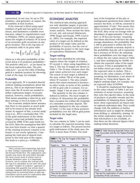
TABLE 1. The Top Ten Targets of the Data
Mining Study*
Target no. Size Area (ha) W-max
1 11.77 144 8.69
2 8.15 136 7.93
3 7.50 148 7.30
4 6.83 134 6.74
5 6.67 133 6.98
6 6.46 134 7.53
7 5.81 146 7.24
8 4.10 90 7.21
9 4.03 86 7.98
10 3.94 90 7.33
*See text for explanation of size, area, and
W-max calculations
area of the footprints of the pits or
underground operations from which this
resource has been, or will be, extracted is
approximately 15 km 2 . This means that,
where economic gold deposits occur in
the EGN, they occur on average with an
abundance of approximately 5 Moz per
km 2 , or 50 Koz per hectare. Assuming
that future discoveries will have the same
average abundance, the probability that
a 100 m grid point is within the footprint
of a mineable economic deposit is
the probability that the cell it represents
has a resource of 50 Koz. By summing
these probabilities over the target area,
to obtain the size values shown in Table
1, and then multiplying by 50,000, we
obtain the expected value of the target
in ounces. If this is multiplied by the
net dollar return per ounce, we obtain
the expected value in dollars. This is
shown in the value column of Table 2
assuming, for illustration, a net return of
$500 per oz. Using these figures, the
highest ranking target, for example, has
an expected value of $294M.
It should be emphasized that figures
in the value column of Table 2 are not
estimates of actual resources, assuming
they exist, but expected values, in the sense
of products of possible rewards and the
probabilities of obtaining them. Further -
more, these expectations are based only
on regional exploration data. They would
change with the addition of further
information such as might be obtained
from drilling or, ultimately, mining. At
the initial exploration stage, however,
that information is not available, so
that these are the relevant figures when
making initial decisions.
TABLE 2. Table Showing Expected Values and
Costs Associated with the Ten Highest Ranked
Targets*
Target Value Cost Prob
no. $M $K %
1 294 720 20.6
2 204 680 13.3
3 187 740 8.9
4 171 670 11.3
5 167 665 10.2
6 161 670 10.4
7 145 730 8.7
8 103 450 8.5
9 101 430 13.7
10 99 450 9.1
Total $1.6B $6.2M
*See text for explanation of value, cost, and
probability (Prob) calculations