SIMPLE Method on Non-staggered Grids - Department of ...

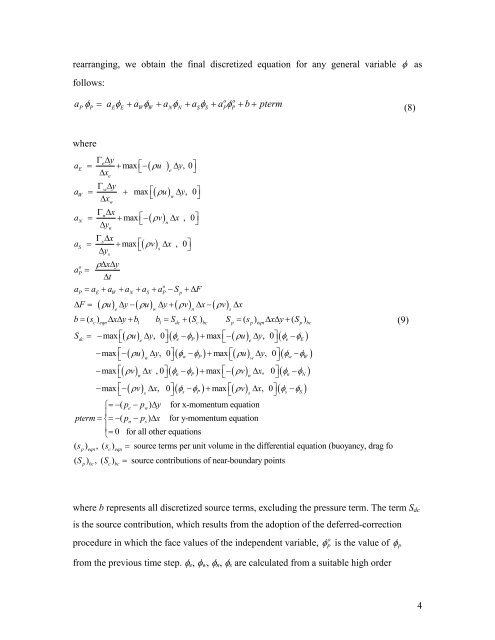
earranging, we obtain the final discretized equation for any general variable φ as
follows:
o o
aPφP = aEφE + aWφW + aNφN + aSφS + aPφP
+ b+ pterm
(8)
where
aE
=
ΓΔ
e
y
+ max ⎡−( ρu ) Δy, 0⎤
e
Δx
⎣
⎦
e
aW
=
ΓΔ
w
y
+ max ⎡( ρu)
Δy, 0⎤
w
Δx
⎣ ⎦
w
aN
=
ΓΔ
n
x
+ max ⎡−( ρv)
Δx
, 0⎤
n
Δy
⎣
⎦
n
aS
=
ΓΔ
s
x
+ max ⎡( ρv)
Δx
, 0⎤
s
Δy
⎣
⎦
s
o ρΔΔ
x y
aP
=
Δt
o
aP = aE + aW + aN + aS + aP − Sp
+ΔF
Δ F = ( ρu) Δy−( ρu) Δ y+ ( ρv) Δx−( ρv)
Δx
e w n s
b= ( sc )
eqn
ΔxΔ y+ b1 b1
= Sdc + ( Sc)
bc
Sp = ( sp) eqnΔxΔ y+
( Sp)
bc
(9)
Sdc = −max ⎡
⎣( ρu) Δy, 0⎤( ) max ( ) , 0 ( )
e ⎦ φe − φP + ⎡
⎣
− ρu Δy
⎤
e ⎦ φe −φE
−max ⎡
⎣
−( ρu) Δy, 0⎤( w P) max ( ) , 0 ( w W)
w ⎦ φ − φ + ⎡
⎣ ρu Δy
⎤
w ⎦ φ −φ
−max ⎡
⎣( ρv) Δx , 0⎤( φn φP) max ( ρv) x, 0 ( φn φN)
n ⎦
− + ⎡
⎣
− Δ ⎤
n ⎦
−
−max ⎡
⎣
−( ρv) Δx, 0⎤( φs − φP) + max ⎡( ρv) Δx, 0⎤( φs −φS)
s ⎦ ⎣ s ⎦
⎧=−( pe
−pw) Δy
for x-momentum equation
⎪
pterm= ⎨=−( pn
− ps) Δx
for y-momentum equation
⎪
⎩ = 0 for all other equations
( s ) , ( s ) = source terms per unit volume in the differential equation (buoyancy, drag for
p eqn c eqn
( Sp) bc, ( S
c) bc=
source contributions of near-boundary points
where b represents all discretized source terms, excluding the pressure term. The term S dc
is the source contribution, which results from the adoption of the deferred-correction
o
procedure in which the face values of the independent variable, φ
P
is the value of φ
P
from the previous time step. φ e , φ w , φ n , φ s are calculated from a suitable high order
4