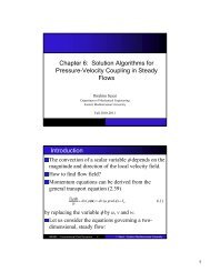
SIMPLE Method on Non-staggered Grids - Department of ...

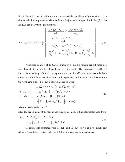
It is to be noted that body-force term is neglected for simplicity of presentation. By a
similar substitution process as the one for the Majumdar’s interpolation in Eq. (21), the
Eq. (22) can be written equivalently as
( 1 )
u ⎡f u f u ⎤
⎣
⎦
( − p ) +
fe
( aP)
e
α Δy( p − p
+
)
e
( a )
⎧ α Δy p
⎪− +
⎪
⎪
⎪+ ( 1−
f )
⎪
( − p )
( a )
u E P u e w E
u e w P
α Δy p
+ +
P P
e
=
e E
+ −
e P
+⎨ ⎬
n− 1 + n− 1 + n−1
( 1 α ) ⎡
u
ue fe uE ( 1 fe ) u ⎤
⎣
P
⎦
o
o
⎡α
α ( a )
+ +
⎢
( 1 )
⎪+ − + − −
⎪
⎪
o
a α ( a
⎪ u f u f
)
+ − − −
u
⎪ ⎢( a ) a a
⎩ ⎣
u e o u P
E o u P
P o
e e E e P
P ( P)
( P)
e E P
P
E
⎫
⎪
⎪
⎪
⎪
⎪
⎪
⎪
⎤⎪
⎥⎪
⎥⎪
⎦⎭
(24)
According to Yu et al. (2002), solutions by using this scheme are still time step
size dependent, though the dependence is quite small. They proposed a different
interpolation technique for the terms appearing in equation (22) which appears to be both
under relaxation factor and time step size independent. In this method the first term on
the right-hand side of Eq. (22) is interpolated as follows:
∑ au + b
( ∑ +
1) + ( 1− )( ∑ + )
E
1
+ +
fe ( sc) ( 1 fe )( sc)
⎤δ
x
E
P e
y
( ∑ ) + ( 1− )( ∑ )
f au b f au b
+ +
e i i i e i i i
+ ⎡ + − Δ
⎛ i i i p ⎞ ⎣ ⎦
⎜ ⎟ =
+ +
⎝ aP ⎠ f
e e i
ai f
E e i
ai
P
where b
1
is defined in Eq. (9).
( ) ( 1 )( )
− ⎡f s + − f s ⎤δ
x Δ y+
a
⎣
⎦
+ +
o
e p
E
e p
P
e e
Also, the denominator of the second and third terms in Eq. (22) is interpolated as follows:
+ +
( a ) = f ( ∑ a ) + ( 1− f )( ∑ a )
P e e i i E e i i P
( ) ( 1 )( )
− ⎡f s + − f s ⎤δ
x Δ y+
a
⎣
⎦
+ +
o
e p
E
e p
P
e e
Equation (22) combined with Eq. (25) and Eq. (26) is Yu et al.’s (2002) new
scheme. Substituting Eq. (25) into Eq. (22) the following equation is obtained:
P
(25)
(26)
8