SIMPLE Method on Non-staggered Grids - Department of ...
SIMPLE Method on Non-staggered Grids - Department of ...
SIMPLE Method on Non-staggered Grids - Department of ...

Create successful ePaper yourself
Turn your PDF publications into a flip-book with our unique Google optimized e-Paper software.
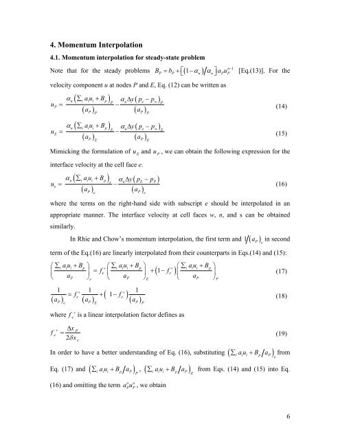
4. Momentum Interpolati<strong>on</strong><br />
4.1. Momentum interpolati<strong>on</strong> for steady-state problem<br />
BP = bP + ⎡⎣ 1−αu αu⎤⎦ aPuP<br />
[Eq.(13)]. For the<br />
n−1<br />
Note that for the steady problems ( )<br />
velocity comp<strong>on</strong>ent u at nodes P and E, Eq. (12) can be written as<br />
u<br />
u<br />
P<br />
E<br />
( )<br />
( a )<br />
P<br />
P<br />
( )<br />
( a )<br />
αu ∑<br />
i<br />
au<br />
i i<br />
+ Bp α<br />
P uΔy pe − pw<br />
P<br />
= − (14)<br />
( )<br />
( a )<br />
P<br />
E<br />
P<br />
P<br />
( )<br />
( a )<br />
αu ∑<br />
i<br />
au<br />
i i<br />
+ Bp α<br />
E uΔy pe − pw<br />
E<br />
= − (15)<br />
Mimicking the formulati<strong>on</strong> <strong>of</strong> u<br />
E<br />
interface velocity at the cell face e.<br />
u<br />
e<br />
( )<br />
( a )<br />
P<br />
e<br />
P<br />
E<br />
and u<br />
P<br />
, we can obtain the following expressi<strong>on</strong> for the<br />
( )<br />
( a )<br />
αu ∑<br />
i<br />
au<br />
i i<br />
+ Bp α<br />
e uΔy pE − pP<br />
= − (16)<br />
P<br />
e<br />
where the terms <strong>on</strong> the right-hand side with subscript e should be interpolated in an<br />
appropriate manner. The interface velocity at cell faces w, n, and s can be obtained<br />
similarly.<br />
In Rhie and Chow’s momentum interpolati<strong>on</strong>, the first term and 1 ( aP ) in sec<strong>on</strong>d<br />
e<br />
term <strong>of</strong> the Eq.(16) are linearly interpolated from their counterparts in Eqs.(14) and (15):<br />
⎛∑ au + B ⎞ ⎛∑ au + B ⎞ ⎛∑ au + B ⎞<br />
⎜ ⎟ ⎜ ⎟ ( 1 fe<br />
) ⎜ ⎟<br />
⎝ ⎠ ⎝ ⎠ ⎝ ⎠<br />
i i i p + i i i p + i i i p<br />
= fe<br />
+ −<br />
aP a<br />
e P<br />
a<br />
E P P<br />
(17)<br />
1 + 1 + 1<br />
= f + − (18)<br />
a a a<br />
e<br />
( ) ( )<br />
( 1 fe<br />
) ( )<br />
P e P E P P<br />
where f + e<br />
is a linear interpolati<strong>on</strong> factor defines as<br />
+ Δx<br />
P<br />
f<br />
e<br />
= (19)<br />
2δ x<br />
e<br />
In order to have a better understanding <strong>of</strong> Eq. (16), substituting ( au B a )<br />
Eq. (17) and ( ∑ au + B a ) , ( au B a )<br />
i i i p P P<br />
o o<br />
(16) and omitting the term au , we obtain<br />
P<br />
P<br />
i i i p P E<br />
∑ + from<br />
i i i p P e<br />
∑ + from Eqs. (14) and (15) into Eq.<br />
6