Assignment 3.pdf - UBC Mechanical Engineering
Assignment 3.pdf - UBC Mechanical Engineering
Assignment 3.pdf - UBC Mechanical Engineering

Create successful ePaper yourself
Turn your PDF publications into a flip-book with our unique Google optimized e-Paper software.
MECH 529<br />
DYNAMIC SYSTEM MODELING<br />
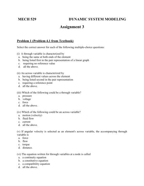
<strong>Assignment</strong> 3<br />
Problem 1 (Problem 4.1 from Textbook)<br />
Select the correct answer for each of the following multiple-choice questions:<br />
(i) A through variable is characterized by<br />
a. being the same at both ends of the element<br />
b. being listed first in the pair representation of a linear graph<br />
c. requiring no reference value<br />
d. all the above.<br />
(ii) An across variable is characterized by<br />
a. having different values across the element<br />
b. being listed second in the pair representation<br />
c. requiring a reference point<br />
d. all the above.<br />
(iii) Which of the following could be a through variable?<br />
a. pressure<br />
b. voltage<br />
c. force<br />
d. all the above.<br />
(iv) Which of the following could be an across variable?<br />
a. motion (velocity)<br />
b. fluid flow<br />
c. current<br />
d. all the above.<br />
(v) If angular velocity is selected as an element's across variable, the accompanying through<br />
variable is<br />
a. force<br />
b. flow<br />
c. torque<br />
d. distance.<br />
(vi) The equation written for through variables at a node is called<br />
a. a continuity equation<br />
b. a constitutive equation<br />
c. a compatibility equation<br />
d. all the above.
(vii) The functional relation between a through variable and its across variable is called<br />
a. a continuity equation<br />
b. a constitutive equation<br />
c. a compatibility equation<br />
d. a node equation.<br />
(viii) The equation that equates the sum of across variables in a loop to zero is known as<br />
a. a continuity equation<br />
b. a constitutive equation<br />
c. a compatibility equation<br />
d. a ode equation.<br />
(ix) A node equation is also known as<br />
a. an equilibrium equation<br />
b. a continuity equation<br />
c. the balance of through variables at the node<br />
d. all the above.<br />
(x) A loop equation is<br />
a. a balance of across variables<br />
b. a balance of through variables<br />
c. a constitutive relationship<br />
d. all the above.<br />
Problem 2 (Problem 4.2 from Textbook)<br />
A linear graph has 10 branches, two sources, and six nodes.<br />
(i) How many unknown variables are there?<br />
(ii) What is the number of independent loops?<br />
(iii) How many inputs are present in the system?<br />
(iv) How many constitutive equations could be written?<br />
(v) How many independent continuity equations could be written?<br />
(vi) How many independent compatibility equations could be written?<br />
(vii) Do a quick check on your answers.<br />
Problem 3 (Problem 4.3 from Textbook)<br />
The circuit shown in Figure P4.3 has an inductor L, a capacitor C, a resistor R, and a voltage<br />
source v(t). Considering that L is analogous to a spring, and C is analogous to an inertia, follow<br />
the standard steps to obtain the state equations. First sketch the linear graph denoting the currents
through and the voltages across the elements L, C, and R by (f l , v l ), (f 2 , v 2 ) and (f 3 , v 3 ),<br />
respectively, and then proceed in the usual manner.<br />
(i) What is the system matrix and what is the input distribution matrix for your choice of<br />
state variables?<br />
(ii) What is the order of the system?<br />
(iii) Briefly explain what happens if the voltage source v(t) is replaced by a current source<br />
i(t).<br />
L<br />
v(t)<br />
C<br />
R<br />
Figure P4.3 An electrical circuit.<br />
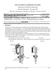
Problem 4 (Problem 4.4 from Textbook)<br />
Consider an automobile traveling at a constant speed on a rough road, as sketched in Figure<br />
P4.4(a). The disturbance input due to road irregularities can be considered as a velocity source<br />
u(t) at the tires in the vertical direction. An approximate one-dimensional model shown in Figure<br />
P4.4(b) may be used to study the “heave” (up and down) motion of the automobile. Note that v 1<br />
and v 2 are the velocities of the lumped masses m 1 and m 2 , respectively.<br />
(a)<br />
(b)<br />
(c)<br />
(d)<br />
Briefly state what physical components of the automobile are represented by the model<br />
parameters k 1 , m 1 , k 2 , m 2 , and b 2 . Also, discuss the validity of the assumptions that are<br />
made in arriving at this model.<br />
Draw a linear graph for this model, orient it (i.e., mark the directions of the branches),<br />
and completely indicate the system variables and parameters.<br />
By following the step-by-step- procedure of writing constitutive equations, node<br />
equations and loop equations, develop a complete state-space model for this system. The<br />
outputs are v 1 and v 2 . What is the order of the system?<br />
If instead of the velocity source u(t), a force source f(t) which is applied at the same<br />
location, is considered as the system input, draw a linear graph for this modified model.<br />
Obtain the state equations for this model. What is the order of the system now?<br />
Note: In this problem you may assume that the gravitational effects are completely balanced by<br />
the initial compression of the springs with reference to which all motions are defined.
(a)<br />
Heave Motion<br />
Forward Speed<br />
(constant)<br />
Reference<br />
Road Surface<br />
(b)<br />
v 2<br />
m 2<br />
k b 2 2<br />
v 1<br />
m 1<br />
u(t)<br />
k 1<br />
Ground Reference<br />
Figure P4.4 (a) An automobile traveling at constant speed<br />
(b) A crude model of the automobile for the heave motion analysis.<br />
Problem 5 (Problem 4.5 from Textbook)<br />
Suppose that a linear graph has the following characteristics:<br />
n = number of nodes<br />
b = number of braches (segments)<br />
s = number of sources<br />
l = number of independent loops.<br />
Carefully explaining the underlying reasons, answer the following questions regarding this linear<br />
graph:<br />
(a) From the topology of the linear graph show that l = b – n + 1<br />
(b)<br />
(c)<br />
What is the number of continuity equations required (in terms of n)?<br />
What is the number of lumped elements including source elements in the model<br />
(expressed in terms of b and s)?
(d)<br />
What is the number of unknown variables, both state and auxiliary, (expressed in<br />
terms of b and s)? Verify that this is equal to the number available equations, and<br />
hence the problem is solvable.<br />
Problem 6 (Problem 4.6 from Textbook)<br />
An approximate model of a motor-compressor combination used in a process control application<br />
is shown n Figure P4.6.<br />
Motor Rotor<br />
T m<br />
Drive Shaft<br />
k<br />
Compressor<br />
T c<br />
J c<br />
J m<br />
ω<br />
m<br />
ω<br />
c<br />
b<br />
m<br />
(viscous)<br />
b<br />
c<br />
(viscous)<br />
Figure P4.6 A model of a motor-compressor unit.<br />
Note that T, J, k, b, and ω denote torque, moment of inertia, torsional stiffness, angular viscous<br />
damping constant, and angular speed, respectively, and the subscripts m and c denote the motor<br />
rotor and compressor impeller, respectively.<br />
(a) Sketch a translatory mechanical model that is analogous to this rotatory mechanical<br />
model.<br />
(b) Draw a linear graph for the given model, orient it, and indicate all necessary variables<br />
and parameters on the graph.<br />
(c) By following a systematic procedure and using the linear graph, obtain a complete<br />
state-space representation of the given model. The outputs of the system are<br />
compressor speed ω c and the torque T transmitted through the drive shaft.<br />
Problem 7 (Problem 4.7 from Textbook)<br />
A model for a single joint of a robotic manipulator is shown in Figure P4.7. The usual notation<br />
is used. The gear inertia is neglected and the gear reduction ratio is taken as 1:r (Note: r < 1).<br />
(a) Draw a linear graph for the model, assuming that no external (load) torque is present<br />
at the robot arm.
(b)<br />
(c)<br />
Using the linear graph derive a state model for this system. The input is the motor<br />
magnetic torque T m and the output is the angular speed ω r of the robot arm. What is<br />
the order of the system?<br />
Discuss the validity of various assumptions made in arriving at this simplified model<br />
for a commercial robotic manipulator.<br />
T m<br />
k<br />
J m<br />
ω<br />
m<br />
ω<br />
r<br />
J r<br />
(viscous)<br />
b m<br />
Motor<br />
1: r<br />
Gear Box (Light)<br />
Robot Arm<br />
Figure P4.7<br />
A model of a single-degree-of-freedom robot.<br />
Problem 8 (Problem 4.8 from Textbook)<br />
Consider the rotatory feedback control system shown schematically by Figure P4.8(a). The load<br />
has inertia J, stiffness K and equivalent viscous damping B as shown. The armature circuit for<br />
the dc fixed field motor is shown in Figure P4.8(b).<br />
(a)<br />
DC Motor<br />
K v , K T<br />
T m<br />
v<br />
Power<br />
r v a<br />
v m<br />
Amplifier<br />
-<br />
K a<br />
J<br />
B<br />
K<br />
Load<br />
Torque<br />
T l<br />
Tachometer<br />
K t<br />
Gear<br />
Ratio r
(b)<br />
i R L<br />
v m<br />
v b<br />
ω = θ<br />
Figure P4.8<br />
(a) A rotatory electromechanical system. (b) The armature circuit.<br />
The following relations are known:<br />
The back e.m.f. vB<br />
= KVω<br />
The motor torque Tm<br />
= Ki T<br />
(a) Identify the system inputs.<br />
(b) Sketch a linear graph for the system, and using that obtain a state-space model for the<br />
system.<br />
Problem 9 (Problem 4.9 from Textbook)<br />
(a) What is the main physical reason for oscillatory behaviour in a purely fluid system?<br />
Why do purely fluid systems with large tanks connected by small-diameter pipes rarely<br />
exhibit an oscillatory response?<br />
(b) Two large tanks connected by a thin horizontal pipe at the bottom level are shown in Figure<br />
P4.9(a). Tank 1 receives an inflow of liquid at the volume rate Q i when the inlet valve is<br />
open. Tank 2 has an outlet valve, which has a fluid flow resistance of R o and a flow rate of<br />
Q o when opened. The connecting pipe also has a valve, and when opened, the combined<br />
fluid flow resistance of the valve and the thin pipe is R p . The following parameters and<br />
variables are defined:<br />
C 1 , C 2 = fluid (gravity head) capacitances of tanks 1 and 2<br />
ρ = mass density of the fluid<br />
g = acceleration due to gravity<br />
P 1 , P 2 = pressure at the bottom of tanks 1 and 2<br />
P 0 = ambient pressure.<br />
Sketch a linear graph for the system. Using P 10 = P 1 – P 0 and P 20 = P 2 – P 0 as the state variables<br />
and the liquid levels H 1 and H 2 in the two tanks as the output variables, derive a complete, linear,<br />
state-space model for the system, systematically from the linear graph.<br />
(c) Suppose that the two tanks are as in Figure P4.9(b). Here Tank 1 has an outlet valve at its<br />
bottom whose resistance is R t and the volume flow rate is Q t when open. This flow directly
enters Tank 2, without a connecting pipe. The remaining characteristics of the tanks are the<br />
same as in Part (b).<br />
Sketch a linear graph for the new system. Systematically derive a state-space model for the<br />
modified system in terms of the same variables as in Part (b), using the new linear graph.<br />
(a)<br />
Inlet Valve<br />
Q i<br />
P 0<br />
Tank 1 Tank 2<br />
P 0<br />
H 1<br />
C 1<br />
Connecting<br />
Valve<br />
H 2<br />
C 2<br />
P 1<br />
Q p<br />
R p<br />
P 2<br />
R o<br />
Outlet Valve<br />
P o<br />
Q o<br />
(b)<br />
Q i<br />
P 0<br />
Tank 1<br />
H 1<br />
C 1<br />
Connecting<br />
Valve<br />
P 1<br />
Q t<br />
R t<br />
Tank 2<br />
P 0<br />
C 2<br />
H 2<br />
P<br />
2<br />
R o<br />
Outlet Valve<br />
P o<br />
Q o<br />
Figure P4.9<br />
(a) An interacting two-tank fluid system.<br />
(b) A non-interacting two-tank fluid system.
Problem 10 (Problem 4.10 from Textbook)<br />
Give reasons for the common experience that in the flushing tank of a household toilet, some<br />
effort is needed to move the handle for the flushing action but virtually no effort is needed to<br />
release the handle at the end of the flush.<br />
A simple model for the valve movement mechanism of a household flushing tank is shown in<br />
Figure P4.10. The overflow tube on which the handle lever is hinged, is assumed rigid. Also, the<br />
handle rocker is assumed light, and the rocker hinge is assumed frictionless.<br />
l h<br />
l v<br />
f(t)<br />
Hinge<br />
(Frictionless)<br />
Handle<br />
(Light)<br />
Lift Rod<br />
Overflow Tube<br />
(Rigid)<br />
x, v<br />
Valve Flapper<br />
(Equivalent mass m)<br />
Valve Damper<br />
(Nonlinear)<br />
Valve Spring<br />
(Stiffness k )<br />
Figure P4.10 Simplified model of a toilet-flushing mechanism.<br />
The following parameters are indicated in the figure:
l<br />
v<br />
= = the lever arm ratio of the handle rocker<br />
lh<br />
m = equivalent lumped mass of the valve flapper and the lift rod<br />
k = stiffness of spring action on the valve flapper.<br />
The damping force f NLD on the valve is assumed quadratic and is given by<br />
f = av v<br />
NLD VLD VLD<br />
where, the positive parameter:<br />
a = a u for upward motion of the flapper (v NLD ≥ 0)<br />
= a d for downward motion of the flapper (v NLD < 0)<br />
with a u >> a d<br />
The force applied at the handle is f(t), as shown.<br />
We are interested in studying the dynamic response of the flapper valve. Specially, the valve<br />
displacement x and the valve speed v are considered outputs, as shown in Figure P4.10. Note<br />
that x is measured from the static equilibrium point of the spring where the weight mg is<br />
balanced by the spring force.<br />
(a) By defining appropriate through variables and across variables, draw a linear graph<br />
(b)<br />
for the system shown in Figure P4.10. Clearly indicate the power flow arrows.<br />
Using valve speed and the spring force as the state variables, develop a (nonlinear)<br />
state-space model for the system, with the aid of the linear graph. Specifically, start<br />
with all the constitutive, continuity, and compatibility equations, and eliminate the<br />
auxiliary variables systematically, to obtain the state-space model.<br />
(c) Linearize the state-space model about an operating point where the valve speed is v .<br />
For the linearized model, obtain the model matrices A, B, C, and D, in the usual<br />
notation. The incremental variables ˆx and ˆv are the outputs in the linear model, and<br />
(d)<br />
the incremental variable f ˆ( t ) is the input.<br />
From the linearized state-space model, derive the input-output model (differential<br />
equation) relating f ˆ( t ) and ˆx .<br />
Problem 11 (Problem 4.11 from Textbook)<br />
A common application of dc motors is in accurate positioning of a mechanical load. A schematic<br />
diagram of a possible arrangement is shown in Figure P4.11. The actuator of the system is an<br />
armature-controlled dc motor. The moment of inertia of its rotor is J r and the angular speed is<br />
ω r . The mechanical damping of the motor (including that of its bearings) is neglected in<br />
comparison to that of the load.<br />
The armature circuit is also shown in Figure P4.11, which indicates a back e.m.f. v b (due<br />
to the motor rotation in the stator field), a leakage inductance L a , and a resistance R a . The<br />
current through the leakage inductor is i L . The input signal is the armature voltage v a (t) as shown.<br />
The interaction of the rotor magnetic field and the stator magnetic field (Note: the rotor field
otates at an angular speed ω m ) generates a “magnetic” torque T m which is exerted on the motor<br />
rotor.<br />
The stator provides a constant magnetic field to the motor, and is not important in the<br />
present problem. The dc motor may be considered as an ideal electromechanical transducer<br />
which is represented by a linear-graph transformer. The associated equations are:<br />
1<br />
ω m = vb<br />
km<br />
Tm<br />
= −kmb<br />
i<br />
where k m is the torque constant of the motor. Note: The negative sign in the second equation<br />
arises due to the specific sign convention used for a transformer, in the conventional linear graph<br />
representation.<br />
The motor is connected to a rotatory load of moment of inertia J l using a long flexible<br />
shaft of torsional stiffness k l . The torque transmitted through this shaft is denoted by T k . The load<br />
rotates at an angular speed ω l and experiences mechanical dissipation, which is modeled by a<br />
linear viscous damper of damping constant b l .<br />
Stator (Constant Field)<br />
v () a<br />
t<br />
+<br />
–<br />
R<br />
a<br />
i<br />
L<br />
L<br />
a<br />
Armature Circuit<br />
i<br />
b<br />
+<br />
v<br />
b<br />
_<br />
Rotor<br />
Tm<br />
ω<br />
m<br />
( k )<br />
m<br />
ω<br />
r<br />
J<br />
r<br />
DC Motor<br />
k<br />
l<br />
T<br />
k<br />
ωl<br />
J<br />
l<br />
Load<br />
b<br />
l<br />
Figure P4.11 An electro-mechanical model of a rotatory positioning system.<br />
Answer the following questions:<br />
(a) Draw a suitable linear graph for the entire system shown in Figure P4.11, mark the<br />
variables and parameters (you may introduce new, auxiliary variables but not new parameters),<br />
and orient the graph.<br />
(b) Give the number of branches (b), nodes (n), and the independent loops (l) in the complete<br />
linear graph. What relationship do these three parameters satisfy? How many independent node<br />
equations, loop equations, and constitutive equations can be written for the system? Verify the<br />
sufficiency of these equations to solve the problem.
(c) Take current through the inductor (i L ), speed of rotation of the motor rotor ( ω r ), torque<br />
transmitted through the load shaft (T k ), and speed of rotation of the load ( ω l ) as the four state<br />
variables; the armature supply voltage v a (t) as the input variable; and the shaft torque T k and the<br />
load speedω l as the output variables. Write the independent node equations, independent loop<br />
equations, and the constitutive equations for the complete linear graph. Clearly show the statespace<br />
shell.<br />
(d) Eliminate the auxiliary variables and obtain a complete state-space model for the system,<br />
using the equations written in Part (c) above. Express the matrices A, B, C, and D of the state<br />
space model in terms of the system parameters R a , L a , k m , J r , k l , b l , and J l only.